A Re-examination of the Distribution of Galactic Free Electrons

Abstract

We present a list of 109 pulsars with independent distance information compiled from the literature. Since the compilation of Frail & Weisberg, there are 35 pulsars with new distance estimate and 25 pulsars for which the distance or distance uncertainty have been revised. We used this data to fit a smooth, axisymmetric, two disk model of the distribution of galactic electrons. The two exponential model components have mean local midplane densities at the solar circle of $2.03\times 10^{-2}\mbox{~{}cm}^{-3}$ and $0.71\times 10^{-2}\mbox{~{}cm}^{-3}$, and scale heights of 1.07 and 0.053 kpc. The thick component shows very little radial variation, while the second has a radial scale length of only a few kiloparsecs. We also examined a model which varies as $\mbox{sech}^{2}(x)$, rather than $\exp(-x)$, in both the radial and vertical direction. We prefer this model with no midplane cusp, but find that the fit parameters essentially describe the same electron distribution. The distances predicted by this distribution have a similar scatter as the more complex model of Taylor & Cordes. We examine the pulsars that deviate strongly from this model. There are two regions of enhanced dispersion measure, one of which correlates well with the Sagittarius-Carina spiral arm. We find that the scatter of the observed dispersion measure from the model is not fit well by either a normal or log-normal distribution of lump sizes, but may be caused instead by the uncertainties in the distances.

1 Introduction

One of the most important discoveries in the study of the interstellar medium is the realization that the warm ionized medium (WIM) is a major component of our galaxy; it has a thick distribution and it is not localized around ionization sources. Reynolds (1989) used the dispersion measures ($\mbox{DM}=\int n_{e}dl$) towards pulsars with known distance to measure the scale height of the WIM in the Milky Way, and showed that it is much larger than that of the bulk of the neutral hydrogen.

If the distance to a pulsar is known, this can be used with its DM to constrain models for the spatial distribution of the free electrons. The most popular model is that derived by Taylor & Cordes (1993, TC), which also used the observed scattering measures to a different set of pulsars to refine the parameters of the model. Their most important contribution was the addition of non-axisymmetric elements, i.e., spiral arms defined by the locations of HII regions (Georgelin & Georgelin 1976). Their main justification is the observed asymmetry in the DM vs. galactic longitude plots. They also incorporated the unusually high DM observed towards the Gum Nebula.

Models of this kind are used frequently to determine distances to pulsars. TC claim that their model yields distances accurate to 25%. But, since its publication, the set of pulsars with independent distance measurement has increased, some distances have been revised, and pulsars with forbidden DM (higher than the asymptotic value predicted by TC) have been observed. In addition, observations of the the angular broadening of radio sources has been used to constrain the electron density in the Galactic center (Lazio et al. 1999; Lazio & Cordes 1998a,b) and the scalelength of the distribution in the anti-center direction (Lazio & Cordes 1998c,d). Finally, the recent completion of the Wisconsin H$\alpha$ Mapper survey of diffuse galactic H$\alpha$ emission with one-degree angular resolution and $\sim 10~{}{\rm km~{}s^{-1}}$ velocity resolution (Reynolds 1998; Haffner 2000) will allow the development of more complex models. These observations will allow for a reassessment of the location of galactic spiral arms (Georgelin & Georgelin 1976; Ruseil et al. 1998; Georgelin et al. 2000), as well as the discovery and placement of large angular-scale HII regions, such as the Gum Nebula.

In this work, we present an updated list of pulsars of known distance. We then use this data to constrain a new axisymmetric model for the free electron distribution, and show how the Taylor-Cordes model and the new axisymmetric model fare in predicting distances to the pulsars. We also consider to what degree the available data constrain the lumpiness of the warm ionized medium. Incorporation of non-axisymmetric effects, such as the galactic spiral arms and individual nebulae can subsequently be incorporated using the WHAM data and more recent radio recombination line surveys of HII regions.

2 The Pulsar Data Set

A list of 109 pulsars with distance information was gathered from a number of sources and are compiled in Table 1, and presented in order of increasing distance. Of this list, four are in the Large or Small Magellanic clouds. Of the remainder, 76 have both upper and lower distance limits; 20 have only lower limits, and 9 have only upper limits. This dataset is $\sim$ 50% larger than the data used by TC. Of the 109 pulsars, there are 35 new distance determinations since the compilation of Frail & Weisberg (1990, FW90), which provided the bulk of the measurements used in the TC model, 25 objects in which there have been revisions in either the distance or distance uncertainty of the pulsar, and 49 objects whose distance estimates remained unchanged.

Distance estimates come from a variety of methods, which we briefly summarize here.

Kinematic distances (68 pulsars): The majority of pulsar distance measurements come from the combination of 21 cm absorption combined with an axisymmetric, kinematical model for galactic rotation (Fich, Blitz, & Stark 1989). FW90 re-evaluated all the distance measurements up to that time using this model (with corrections for pulsars towards the Perseus arm), and a uniform set of criteria for converting absorption velocities to distance. These criteria have been adhered to in subsequent work. Probably the largest source of systematic error is due to the non-circular “streaming” motions in the vicinity of spiral arms.

Association with globular clusters (17 pulsars): The next most common distance determination method come from association of a pulsar with a globular clusters of known distance. Table 1 only lists one pulsar per globular cluster; when more than one pulsar is known, the variation in dispersion measure is small. Since the compilation of FW90, the distances to globular clusters have been considerably refined due to improved color-magnitude diagrams and shifts in the assumptions about the luminosity of RR Lyrae stars. As a result, some distances estimates have been revised by more than a factor of two since FW90 (Harris 1996, with online updates at http://physun.mcmaster.ca/$\sim$harris/mwgc.dat). The uncertainty in the distance modulus of these clusters was assumed to be $\sigma=0.1+0.4E_{B-V}$ magnitudes. More heavily reddened clusters have poorer data since they have greater problems with field contamination and crowding (Harris 1999).

Association with supernova remnants (10 pulsars): There have been numerous suggested associations between pulsars and supernova remnants (Lorrimer 1998; Gaensler & Johnston 1995; Frail, Goss, & Whiteoak 1994; Kaspi et al. 1996) . However, such associations are hard to prove, since they depend upon expectations for supernova remnant lifetimes, pulsar ages, and transverse velocities. In this compilation, we use the associations judged by Lorrimer, Lyne, and Camilo (1998) to be the “most likely” pulsar-supernova remnant pairs. The only other pulsar/SNR associations added were B1800-21 with G8.7-0.1 (Finley & Ögelman 1994) and B1758-23 with W28 (Frail, Kulkarni, & Vasisht 1993). Both of those have independent kinematic distances which support the association.

Trigonometric parallax (8 pulsars): Potentially the most reliable distances come from interferometric measurements of annual parallax. However, there are several practical difficulties arising from ionospheric effects and a scarcity of nearby calibrators for positions. Improvements in the techniques have led to changes in the published distances by more than a factor of two. The distance estimate for B0950+08 increased from 130 pc (Gwinn et al. 1986) to 280 pc (Brisken et al. 2000), while the distance estimate for B1919+06 decreased from 3.3 kpc (Fomalont et al. 1999) to 1.2 kpc (Chatterjee et al 2000). These changes were much larger than the stated uncertainties in the measurements. Accurate estimates are vital if pulsars are to be used as probes of the structure of the local interstellar medium.

Association with other galaxies (4 pulsars): Four pulsars have been associated with the Magellanic Clouds, three in the LMC, one in the SMC. These pulsars are valuable in constraining the electron density in the Galactic halo. However, an unknown fraction of the dispersion measure must arise in the host galaxy, so their utility in constraining the Galactic free electron column density is compromised.

Timing parallax (5 pulsars): Distances to millisecond pulsars have also been estimated using variations in arrival time of the pulses. There is a annual change in the pulse arrival time whose magnitude is given by $\Delta t=r^{2}cos^{2}\theta/(2cd)$ where r is the Earth-Sun distance, $\theta$ is the angle between the line of sight and the ecliptic plane, and $d$ is the distance (Ryba & Taylor 1991). This variation is $\Delta t=1.2\mu$ sec for $d=$ 1 kpc. This level of timing accuracy has been reached for only a few pulsars.

Period derivative distances (2 pulsars): Bell & Bailes (1996) have shown that in many cases, the observed orbital period derivative of binary pulsars is dominated by term of the form $\dot{P}_{b}/P_{b}=v^{2}/(cd)$. If one uses the predictions of general relativity to derive the intrinsic period derivative, knowledge of the proper motion of the pulsar then allows for an accurate estimate of the distance. This method has only been applied to two pulsars to date.

Spectroscopic parallax of binary companion (1 pulsar): There is one case in which the binary companion of a pulsar is a $\sim$ 10 $M_{\sun}$ Be star (Johnston et al. 1994). In this case, spectroscopic parallax was used to estimate the distance.

X-ray luminosity distance (1 pulsar): There is one distance estimate for B0656+14 based upon the identification of the X-ray counterpart together with a model of thermal X-ray emission from the neutron star (Golden & Shearer 1999). As will be seen, this pulsar ends up being an outlier in our model. As a result, we are not convinced that this method is reliable.

Trigonometric parallax of optical counterpart (0 pulsars): If the optical counterpart of a pulsar can be identified, then ground based or Hubble Space Telescope observations could yield a parallax estimate. This technique has been used to determine the distance to the neutron star Geminga (Caraveo et al. 1996). However, we have not included Geminga in our list because it is unclear if it has a reliable radio signal. The search for optical counterparts of pulsars has been relatively unsuccessful to date (Caraveo 2000). Still, we think this method holds some promise, particular for pulsars with the very lowest dispersion measures like J0108-1431 which has $DM=1.83~{}{\rm cm^{-3}~{}pc}$ (Tauris et al. 1994).

Scattering screen distance (0 pulsars): It has been suggested that the transverse velocity of a pulsar derived using models of interstellar scintillation can be combined with measurements of proper motion to constrain the distance to the pulsar (Gupta 1995; Deshpande & Ramachandran 1998; Cordes & Rickett 1998). Application of this model requires a knowledge of the distribution of electron density and scattering properties along the line of sight, and as a result is principally useful for pulsars which lie behind HII regions of known distance or pulsars well above the disk of the Galaxy.

Cross-checks (7 pulsars): There are six pulsars for which two independent methods have been applied for distance determination. In each case, the distances estimate agree within the stated errors, although in two cases the agreement is marginal. Such checks are important since they test the reliability of the individual methods. We summarize these results here. B1929+10: This pulsar has three discrepant measures for trigonometric parallax, $\pi=21.5\pm 0.3$ mas (Salter, Lyne, & Anderson 1979), $\pi<4$ mas (Backer & Sramek 1982), and $\pi=5.0\pm 1.5$ mas (Campbell 1995). The kinematic distance is $d<1.6$ kpc (Weisberg, Rankin, & Boriakoff 1987). We have adopted the most recent parallax distance, which is consistent with the kinematic distance. B0833-45: The distance to the Vela SNR is given as $d=250\pm 30$ pc (Cha, Sembach, & Danks 1999), while recent VLBI parallax gives $d=316^{+37}_{-29}$ pc (Legge 2000). While these uncertainties do not overlap, the uncertainties in stellar distances may be slightly underestimated. B1855+09: Timing parallax distance to this pulsar was given as $d=0.83^{+0.66}_{-0.24}$ pc (Ryba & Taylor 1991), later refined to $d=0.91^{+0.34}_{-0.20}$ pc (Kaspi, Taylor, & Ryba 1994). This agrees marginally well with the kinematic distance limits $d_{lower}=1.6\pm 0.5$ to $d_{upper}=2.0\pm 0.4$ (Kulkarni, Djorgovski, & Klemola 1991). B1800-21: The kinematic distance limits to this pulsar are $d_{lower}=4.0\pm 0.6$ kpc and $d_{upper}=4.9\pm 0.3$ kpc which agree with the kinematic distance to the SNR G8.7-0.1, also established kinematically (Finley & Ögelman 1994). B1758-23: The kinematic distance limits to this pulsar are $d_{lower}=3.5\pm 0.9$ kpc and $d_{upper}=6.9\pm 0.1$ kpc which agree with the kinematic distance to W28, also established kinematically (Frail, Kulkarni, & Vasisht 1994). B1937-21: Kinematic distance limits are $d_{lower}=4.6\pm 1.9$ kpc and $d_{upper}=14.8\pm 0.9$ kpc (Heiles et al. 1983), which agrees with the timing parallax distance of $d>3.6$ kpc (Kaspi, Taylor, & Ryba 1994). B1534+12: The period derivative distance to this binary pulsar is $d=1.08\pm 0.15$ kpc, which is consistent with the timing parallax limit of $d>0.67$ kpc (Stairs et al. 1999)

Figure 1 shows the spatial distribution of the pulsars in our sample with both upper and lower distance limits projected onto the Galactic plane, while Figure 2 shows a plot of their dispersion measure as a function of galactic longitude. Note that in Figure 2, there is no clear evidence for the asymmetry in maximum dispersion measure around $l=0^{\circ}$, which is present in the complete set of pulsars including those of unknown distance.

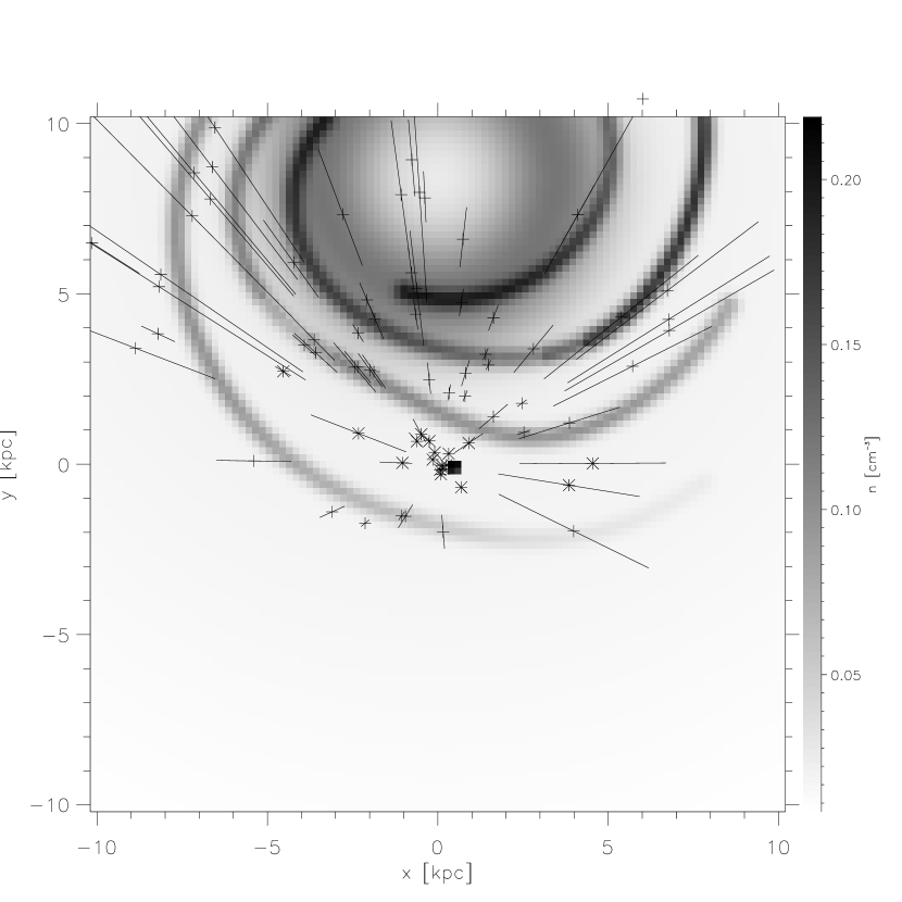
Figure 1: Projection of the position of the pulsars onto the galactic plane. Uncertainties in the distance from the Sun are also shown. The location and density of the spiral arms, central annulus and Gum Nebula in the Taylor-Cordes model are noted in grey-scale. Pulsars marked with a star are the ones considered in the “interarm direction” as seen from the Sun, although this neglects the potential contribution of the Local Arm.

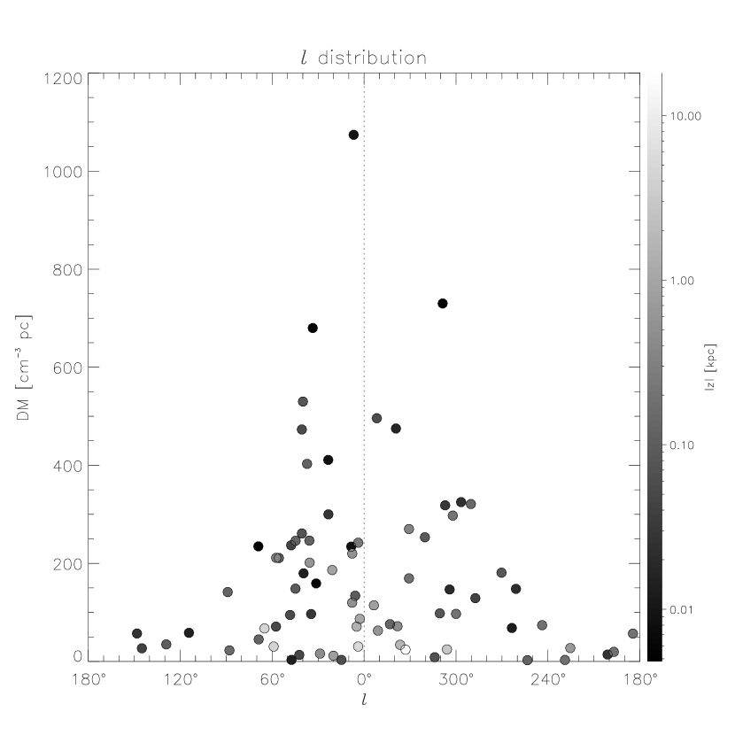
Figure 2: Distribution of the pulsar dispersion measure with galactic longitude. Grayscale indicates their distance from the galactic midplane. In this data set, there is no clear evidence for an asymmetrical distribution with galactic longitude.

3 Fitting an axisymmetric model

Using this data, we fit a two component model of the galactic disc to the pulsar data. The model has the form,

$$n_{e}(r,z)=n_{0}\frac{f(r/r_{0})}{f(r_{\sun}/r_{0})}f(z/z_{0})+n_{1}\frac{f(r/r_{1})}{f(r_{\sun}/r_{1})}f(z/z_{1}),$$

where $f(x)$ is either $=\exp(-x)$ or $=\mbox{sech}^{2}(x)$, and $r_{\sun}=8.5\mbox{~{}kpc}$ is the galactocentric distance of the Sun. The fit was achieved through a variant of the $\chi^{2}$ method: we defined the error-of-the-fit $\Delta$ as,

$$\Delta=\frac{1}{n-\nu}\sum\frac{\log^{2}(\mbox{DM}_{data}/\mbox{DM}_{model})}{\sigma^{2}+\sigma_{A}^{2}},$$

where $n$ is the number of pulsars (76) with both upper and lower distance limits, $\nu$ is the number of free parameters in the model (6), $\mbox{DM}_{data}$ are the observed DM’s, $\mbox{DM}_{model}$ is the modeled DM’s, obtained by integrating the model through the line of sight to each pulsar position, $\sigma=0.5\log(D_{max}/D_{min})$,$D_{max}$ and $D_{min}$ are the one sigma distance brackets, $\sigma_{A}=0.5\log[(1+A)/(1-A)]$ and $A$ is a noise parameter. The form of this extra term comes from assuming that there is extra error proportional to the dispersion measure, i.e,

$$\mbox{DM}_{A}=\mbox{DM}_{model}(1\pm A)$$

$$\sigma_{A}=0.5\log(\mbox{DM}_{A+}/\mbox{DM}_{A-}).$$

Most of the distances to the pulsars we used (41 out of 76) are determined by assuming a kinematic model for the galactic rotation and comparing it to the 21 cm absorption observed towards the pulsar. For these pulsars, we define the distance to be halfway between the minimum and maximum limits. For these pulsars, there is a uniform probability for the location of the pulsar between the distance brackets, as opposed to the distances obtained by parallaxes, for example, which have a gaussian probability distribution for the distance around a preferred value. Therefore, the kinematic distances have an extra $1/\sqrt{3}$ factor in the corresponding $\sigma$.

An annealing procedure was used to get the best fit for the $n_{0,1},r_{0,1}$ and $z_{0,1}$ parameters with $A=0$. Then, $A$ was adjusted to get $\Delta=1$ and a new fit was obtained. The procedure was repeated until convergence was achieved. Outlier pulsars were spotted by a procedure described below, and those common to both functional forms were taken out of the sample. Then, the procedure was repeated and the new fit is the one considered as final. The parameters of the best fits are in Table 2. The results of the fits for the $f(x)=\mbox{sech}^{2}(x)$ case is presented in Figure 3. The corresponding density profiles are shown in Figure 4. There is not enough data to distinguish between the two functional forms, but the resulting fit parameters are different in each case. We prefer the $\mbox{sech}^{2}(x)$ model because it does not have a midplane cusp, and yields fewer outliers. For this case:

$$n_{e}(r,z) = 1.77\times 10^{-2}\mbox{~{}cm}^{-3}~{}\frac{\mbox{sech}^{2}(r/15.4\mbox{~{}kpc})}{\mbox{sech}^{2}(R_{\odot}/15.4\mbox{~{}kpc})}~{}\mbox{sech}^{2}(z/1.10\mbox{~{}kpc})$$

$$+ 1.07\times 10^{-2}\mbox{~{}cm}^{-3}~{}\frac{\mbox{sech}^{2}(r/3.6\mbox{~{}kpc})}{\mbox{sech}^{2}(R_{\odot}/3.6\mbox{~{}kpc})}~{}\mbox{sech}^{2}(z/0.04\mbox{~{}kpc})$$

These results are comparable to the previous axisymmetric model of Cordes et al. (1991), although our thin disk component has a lower midplane density ($n=10^{-2}~{}{\rm cm^{-3}}$ vs. $n=20\times 10^{-2}~{}{\rm cm^{-3}}$) and a shorter scaleheight ($h=40$ pc vs. $h=175$ pc). We also find a noise parameter of $A=0.30$. Savage et al. (1990) did a similar study with a smaller sample of pulsars. The value of the exponential scale height found is consistent with theirs within the error bars, but their intrinsic scatter ($1.65=1+A$) is larger than ours.

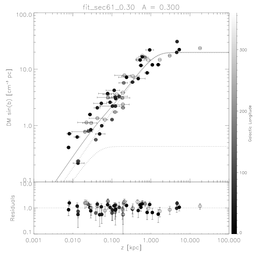
Figure 3: [Upper panel] DMsin(b) as a function of z for the pulsars used in fitting our final model. The solid line shows the two component model with $f(x)=\mbox{sech}^{2}(x)$ at the solar radius. The dotted line shows the two individual components. The error bars show only the effects of distance uncertainty and do not incorporate the noise parameter. [Lower panel] The residual values for our fit, defined as $\mbox{DM}_{data}/\mbox{DM}_{model}$. The uncertainties incorporate the effects of our noise parameter, $A=0.30$. No clear trend in the residuals with galactic longitude (shown in grayscale) is observed.

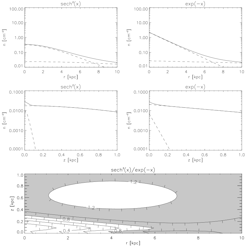
Figure 4: Resulting density distributions, and comparison of the two functional forms. Dashed lines show the individual components and the solid lines show the sum. Upper panels shows midplane density versus galactocentric radius. Middle panel shows $n(z)$ for $r=r_{\sun}=8.5\mbox{~{}kpc}$. The lower panel shows ratio of the two model densities versus $r$ and $z$. The pulsar dataset cannot distinguish between the two functional forms. The shaded region shows where the predicted electron density of the two models differ by less than 20%.

The procedure for spotting the outliers was the following: Consider the values of $\mbox{DM}_{model}$ obtained by integrating $n_{e}$ in the line of sight towards each pulsar to the distance brackets, and call them $\mbox{DM}_{+}$ and $\mbox{DM}_{-}$. Consider now the values,

$$x_{\pm}=\frac{\mbox{DM}_{data}}{\mbox{DM}_{model}}\pm\sqrt{\left(\frac{\mbox{DM}_{model}-\mbox{DM}_{\pm}}{\mbox{DM}_{model}}\right)^{2}+A^{2}},$$

for each pulsar (the error bars in the bottom panel of Figures 5 and 6 are the values of the square root above). If $\mbox{sign}(x_{+}-1)=\mbox{sign}(x_{-}-1)$, then that pulsar is considered an outlier. As mentioned, the pulsars spotted as outliers for both functional forms are taken out of the sample for the final calculation of the fit.

4 Deviations from the Smooth Axisymmetric Model

Since observations of HII regions in the Galaxy show that there are clearly inhomogeneities and asymmetries in the distribution of free electrons, we have looked for patterns in the spatial and statistical distribution of our residuals, $DM_{data}/DM_{model}$. We discuss in turn, the individual outliers, the distribution of residuals with respect to longitude and distance, and the nature of the scatter about our smooth model. In the future, the combination of this data with new radio recombination surveys for distant HII regions and velocity-resolved $H\alpha$ surveys of more nearby gas will yield a more complicated, but realistic, model.

4.1 Outliers

Of the 76 pulsars with both upper and lower limits, 15 are outliers in both the exponential and $\mbox{sech}^{2}(x)$ model. These outliers are noted in Table 3, together with the observed dispersion measure, and the dispersion measure that we would predict given the distance, $DM_{\pm}=(1\pm A)DM_{model}(D)$. Two of these pulsars have dispersion measure that are lower than one would expect given their distance. The first, B1741-11, with a timing parallax distance, is only 0.36 kpc distant. Given the lumpiness of the local interstellar medium (Cox & Reynolds 1987; Toscano et al. 1999), it is not out of the question for such a low density sightline to arise for such a short distance. The second pulsar with a much lower dispersion measure than expected is B1937+21. This pulsar, which has a kinematic distance of $d=4.6$ kpc to 14.6 kpc, has $DM=71~{}{\rm cm^{-3}~{}pc}$, while our model yields $DM_{-}=208~{}{\rm cm^{-3}~{}pc}$. This yields a mean of electron density of $n_{e}<0.016~{}{\rm cm^{-3}}$ over at least a 4.5 kpc pathlength! Further timing parallaxes for this pulsar could confirm this unusual result.

While low DM outliers are difficult to explain, high DM outliers are likely to arise due to the passage the pulsar line of sight through a dense HII region. Of the 13 high outliers, four are associated with SNR (Vela, MSH 15-52 SNR, G308.8-0.1, and W28) and one has a 10 $M_{\sun}$ companion (and presumably an associated HII region). Using the ionizing output luminosity tabulated in Osterbrock (1989), the dispersion measure of an HII region around an O9 star, for example, would be $DM=2nR_{S}=315~{}{\rm cm^{-3}pc}$, where $R_{S}$ is the Strömgren radius. The excess dispersion measure, defined as $DM_{excess}=DM_{data}-DM_{+}$ for the 13 high outliers range from $DM_{excess}=7-578~{}{\rm cm^{-3}pc}$. Thus these lines of sight are consistent with the intersection of the line of sight with discrete HII regions. However, we have searched catalogs of diffuse HII regions (Lockman, Pisano, and Howard 1996) and the WHAM maps (Haffner 2000) for correlations with these northern declination pulsars in this sample, but nothing outstanding was found. Since the majority of these pulsars lie at southern declinations, the high angular resolution $H\alpha$ maps of Gaustad et al. (1997) will be extremely useful in the future.

There are two outliers for which we suspect the distance estimate may be incorrect. The distance to B0656+14 was obtained using an X-ray luminosity distance. Given the number of assumptions necessary to estimate the X-ray luminosity of a neutron star, we have some concerns about the reliability of this method. The distance to B0823+26 is based on a parallax measurement by Gwinn et al. (1986). Since the other pulsar examined in this study (B0950+08) has had a significant revision in its distance, a reconsideration of this pulsar parallax may be in order.

We have also compared to the 29 pulsars for which there are only upper or lower limits. We found that 26 of the limits are satisfied by the model while B2020+28 ($D>3.1$ kpc), B2016+28 ($D>3.2$ kpc), and B1818-04 ($D<1.6$ kpc) are not. Thus our model satisfies the distance constraints of 91 out of 109 pulsars.

4.2 Spatial Distribution of Residuals

We now consider whether the known asymmetries in the distribution of galactic HII regions is reflected in the current dataset. A plot of $\mbox{DM}_{data}/\mbox{DM}_{model}$ versus galactic location is presented in Figure 5, with the spiral arm positions used by TC overlaid. There seem to be two lines of pulsars with a higher than expected dispersion measure, marked by dashed lines. Some of these pulsars have been discussed by Johnston et al. (2001) as particularly noticeable outliers. One of these groups agrees roughly with the position of one of the spiral arms and has a pitch angle $27^{\circ}$ from the tangent. The other has a pitch angle of $22^{\circ}$ and is not coincident with any of the spiral arms. Given the distance uncertainties for these pulsars, it seems clear that any spiral structure that might exist is only weakly exhibited in this data set.

Figure 5: $\mbox{DM}_{data}/\mbox{DM}_{model}$ ratio (values shown via legend symbol) for pulsars with $|z|<300\mbox{~{}pc}$ projected on the Galactic plane. The grid circles are labeled with distance from the Sun. The solid lines trace the center of the spiral arms in the TC model. Pulsars which are identified as outliers in Table 3 have filled symbols. There are two regions of high $\mbox{DM}_{data}/\mbox{DM}_{model}$, at approximately 2 and $5\mbox{~{}kpc}$ from the Sun towards the galactic center. One of these regions (noted with dashed lines) coincides with the position of the Sagittarius-Carina arm.

We have also considered whether there is evidence for a difference in the estimated midplane density if we use only pulsars identified as “interarm pulsars” to estimate the midplane density at the solar neighborhood, where those pulsars are marked as such in Figure 1. We found that there was a slight decrease in the derived midplane density, a factor of $2/3$, compared to the total dataset. However, some of these pulsars may lie in or beyond the Local Arm, which although not included in the TC model, is known to exist in the $H\alpha$ data (Reynolds 1983).

4.3 Constraints on Clumpiness

We now consider what factors affect the scatter in the relationship between our simple axisymmetric model and the observed data. Figure 6 shows the comparison between the $\mbox{DM}_{model}$ and $\mbox{DM}_{data}$. $\mbox{DM}_{model}$ takes into account the geometry of the distribution, so it measures the effective integration path. Therefore, we will use it instead of the distance in order to examine the nature of the scatter. An interesting feature in this plot is that the scatter appears to be a fixed fraction of the total dispersion measure.

Figure 6: $\mbox{DM}_{data}$ vs. $\mbox{DM}_{model}$ for the best fit model with $f(x)=\mbox{sech}^{2}(x)$. The starred points are the pulsars identified as outliers. The error bars shown here only show the uncertainties in the distances and do not incorporate our parameterization of scatter in the relationship.

We considered the possibility that the scatter of $\mbox{DM}_{data}$ about the smooth model might derive from a patchiness of the distribution of electrons in the Galaxy. Such a patchiness of the diffuse ionized medium has been predicted, for example, by Miller & Cox (1993) using the observed locations of O stars in the Solar Neighborhood, and a model for the ISM distribution, to calculate the steady state Strömgren volume distribution and ionization.

What would happen if the warm ionized medium were purely located in discrete lumps (or HII regions)? In that case, we define $\widehat{DM}=DM_{model}$ as the dispersion measure that would result for the average line of sight through some variable number of clumps. The expected total number of lumps intersected along a line of sight would then be $n=\widehat{DM}/DM_{lump}$. The variance in observed number should also be $n$ so that $(DM_{data}-\widehat{DM})^{2}=nDM_{lump}^{2}=\widehat{DM}\cdot DM_{lump}$. We can therefore define a quantity, $\mu$, for each pulsar,

$$\mu=\frac{(\mbox{DM}_{data}-\widehat{DM})^{2}}{\widehat{DM}}~{}.$$ (1)

If the lump sizes are normally distributed, $\mu$ should be independent of $\widehat{DM}$, and its average over a large enough sample of pulsars should be the dispersion measure of the lump. In Figure 7 we plot the running mean of this quantity for both the top-down (from large $DM_{model}$ to small $DM_{model}$) and bottom-up sums. There is a strong trend in the lump size estimator with the distance. This could be explained by having two lump populations: small frequent lumps and large rarer lumps. Nearby, we pick only small lumps, yielding a small mean. As we move farther, we pick up more large lumps and the mean value increases. This could explain the steps observed in the bottom-up running mean, while the top-down running mean is flatter. We thought that a log-normal distribution with the appropriate shape parameter might have that property, but found that a log-normal distribution could almost reproduce the properties of Figure 5 (constant fractional scatter with increasing DM), but not Figure 7 ($\mu$ is not constant).

Figure 7: Estimation of the mean lump size. The top-down (dashed) and bottom-up (dotted) running averages are shown. If the variance where due to random encounter of lumps along the line of sight, the average of the ordinate should be constant, independent of DM, and roughly equal to the lump size. The solid line is the least-squares fit to the logarithm of the data.

Another possibility is that the deviations of the observed and modeled DM are not due to statistical noise, but instead fractional errors in the distance measurements. In such case, the variance is proportional to $f^{2}\widehat{DM}^{2}$, where $f$ is the approximate fractional error, rather than $\sqrt{n}DM_{lump}$. In this case, a plot of $(\widehat{DM}-\mbox{DM}_{data})^{2}/\widehat{DM}^{2}$, should be roughly flat, which is verified in Figure 8. The corresponding value is $f\cong 30\%$. If distance uncertainties are indeed the main source of scatter, it will be difficult to say anything definitive about the lumpiness of the warm ionized medium based on this type of data.

Figure 8: Estimation of the square of the mean fractional error. The top-down (dashed) and bottom-up (dotted) running averages are shown. The solid line is the least-squares fit to logarithm of the data. Since the slope is close to zero, this implies that the dispersion is approximately a constant fraction of DM. We suspect that this behavior is due principally to distance uncertainties.

5 Predicting Pulsar Distances

One of the principal uses for a model of the galactic free electron distribution model is to predict the distance to pulsars. While we have not yet introduced the effects of asymmetries, spiral structure, and individual H II regions, we have written two FORTRAN routines (one for each functional form tested) that calculate pulsar distances using the model parameters in Table 2. A comparison of the model distances and true distances for our sample of pulsars is given in Figure 9, using the $f(x)=\mbox{sech}^{2}(x)$ model. The error bars are obtained by calculating the distance that corresponds to $(1\pm A)DM_{data}$. We note that no pulsars have a DM higher than the asymptotic limit when the uncertainty associated with our noise parameter $A$ is considered.

Figure 9: Comparison of the predicted and measured distances using the $f(x)=\mbox{sech}^{2}(x)$ model. The horizontal axis is the pulsar number, sorted by distance. The gray region is the quoted range in measured distances. The starred points are the outlier pulsars identified in Table 3, and the error bars include the effect of the noise parameter, $A=0.3$.

In Figure 10, we compare the distances predicted by the TC model and our model with the observed distance constraints. When we consider only those pulsars with allowed DM (smaller than the asymptotic value), the dispersion in our model is similar to the model of TC, but with fewer free parameters.

Figure 10: Comparison of the predicted and measured distances using both our $f(x)=\mbox{sech}^{2}(x)$ model and the Taylor-Cordes model. The horizontal error bars are computed by estimating the distance corresponding to values of $\mbox{DM}=(1\pm A)\mbox{DM}_{data}$. The dispersion in our model is similar to the TC model, despite the fact that we have nine fewer adjustable parameters.

We note however that the model we have developed is relatively unconstrained for pulsars interior to a galactocentric radius of $R\sim 4$ kpc and exterior to 12 kpc. For example, unlike Taylor & Cordes, we have not included a annulus of electron density at $R=4$ kpc, which presumably would be associated with the molecular ring. Lazio & Cordes (1998a,c) have discussed how additional information can be used to constrain these regions. We intend to address these issues in the future when we address the non-axisymmetric structure using the Wisconsin H$\alpha$ Survey.

6 Conclusions.

A smooth model for the distribution of galactic free electrons was obtained from a set of 109 pulsars with independent distance information. Although a more complex model incorporating spiral arms might be possible, we do not think that it is well constrained by this pulsar data alone, so we chose to use a simpler and probably more robust functional form. The exponential scale height obtained is consistent with the value quoted in Reynolds (1996). The scatter parameter found ($A=0.3$) is smaller than the one found by Savage et al. (1990). This scatter parameter is used to predict a range of confidence in the predicted distances to pulsars.

Of pulsars with both upper and lower distance limits, fifteen pulsars are identified as outliers, with thirteen of these showing excess dispersion measure. Some of these are associated with supernova remnants or known HII regions. There is one very unusual pulsar, $B1937+21$, with an extremely low dispersion measure given its distance. In examining the residuals, we identified two regions of enhanced electron density, one of which corresponds well with the expected position of the Sagittarius-Carina spiral arm.

We found that a simple probabilistic model for a lumpy WIM failed to reproduce the deviations of the observed data from the smooth model. We suspect that the main source of scatter in our model is due to distance uncertainties, although it seems clear that are also occasionally large anomalous dispersion measures associated with HII regions. Some of these are in spiral arms, but their distribution may not be uniform in these arms.

Table 1: Pulsars with independent distance information

PSR	l	b	DM	$D_{min}$	D	$D_{max}$	$\frac{<n_{e}>}{10^{-3}}$	Method	Refs
$0435-47\tablenotemark{*}$	253.40	-42.00	2.60	0.16	0.18	0.21	14.4	PDD	46
$0656+14\tablenotemark{*}$	201.11	8.26	14.02	0.12	0.18	0.23	77.9	X	49
$1929+10\tablenotemark{\textdagger}$	47.38	-3.88	3.18	0.15	0.20	0.29	15.9	${\bf\Pi}$,K	5,8,17,27,28,39
$0833-45\tablenotemark{\textdagger}$	263.55	-2.79	68.20	0.22	0.25	0.28	272.8	Vela SNR,$\Pi$	47,58
$0950+08\tablenotemark{\textdagger}$	228.90	43.70	3.00	0.25	0.28	0.31	10.7	$\Pi$	30,52
$1741-11\tablenotemark{*}$	14.79	9.18	3.14	0.33	0.36	0.39	8.7	TP	51
$0823+26$	197.00	31.70	19.50	0.29	0.36	0.45	54.2	$\Pi$	30
$1451-68$	313.90	-8.50	8.60	0.40	0.45	0.53	19.1	$\Pi$	33
$1855+09\tablenotemark{\textdagger}$	42.29	3.06	13.31	0.71	0.91	1.25	14.6	TP, K	23, 34, 38
$2021+51\tablenotemark{*}$	87.86	8.38	22.58	0.76	1.05	1.72	21.5	$\Pi$	42
$1534+12\tablenotemark{*}$	20.00	47.80	11.62	0.93	1.08	1.23	10.8	PDD,TP	50
$1259-63\tablenotemark{*}$	304.2	-0.992	146.72	0.60	1.10	1.60	133.4	SP	59
$1711+07\tablenotemark{*}$	28.75	25.22	15.99	0.83	1.11	1.67	14.4	TP	37
$0919+06\tablenotemark{*}$	225.42	36.39	27.31	1.04	1.20	1.43	22.7	$\Pi$	53,48
$0355+54$	148.20	0.80	57.00	1.40	1.80	2.20	31.7	K	11,12,15
$0329+54$	145.00	-1.20	26.80	1.70	1.85	2.00	14.5	K	1,2,3,9,15,24
$0531+21$	184.56	-5.78	56.79	1.50	2.00	2.50	28.4	Crab SNR	25
$1358-63\tablenotemark{*}$	310.60	-2.10	98.00	1.60	2.15	2.70	45.6	K	43
$1620-26\tablenotemark{\textdagger}$	350.98	15.96	62.86	1.97	2.20	2.46	28.6	NGC 6121 (M4)	56,60
$1740-53\tablenotemark{*}$	338.20	-11.90	71.80	2.12	2.30	2.49	31.2	NGC 6397	56,55,61
$1951+32$	68.77	2.82	44.98	1.00	2.50	4.00	18.0	CTB80 SNR	29
$1807-24\tablenotemark{*}$	5.80	-2.20	134.00	2.17	2.60	3.11	51.5	NGC 6544	56,55,62
$1054-62\tablenotemark{\textdagger}$	290.30	-3.00	321.00	2.50	2.70	2.90	118.9	K	18,22,40
$0138+59$	129.10	-2.10	34.80	2.60	2.75	2.90	12.7	K	12
$1706-44\tablenotemark{*}$	343.10	-2.70	76.00	2.40	2.80	3.20	27.1	K	40
$1853+01$	34.56	-0.50	96.70	2.70	3.30	3.90	29.3	W44 SNR	26
$1900+01$	35.70	-2.00	246.40	2.80	3.40	4.00	72.5	K	16
$2334+61\tablenotemark{*}$	114.28	0.23	58.38	3.00	3.40	3.80	17.2	G114.3+0.3 SNR	45
$1900+05$	39.50	0.20	179.70	3.10	3.70	4.30	48.6	K	24
$1859+07$	40.60	1.10	261.00	2.80	3.75	4.70	69.6	K	21
$0835-41\tablenotemark{\textdagger}$	260.90	-0.30	148.00	1.80	3.90	6.00	37.9	K	13,43
$1910-59\tablenotemark{*}$	336.5	-25.60	34.00	3.79	4.00	4.22	8.5	NGC 6752	56,55,63
$1046-58\tablenotemark{*}$	287.40	0.60	129.00	2.50	4.05	5.60	31.9	K	43
$1509-58$	320.32	-1.16	253.20	3.50	4.40	5.30	57.5	MSH15-52 SNR	26
$1800-21$	8.40	0.10	234.20	4.00	4.45	4.90	52.6	K,G8.7-0.1 SNR	24,57
$0740-28\tablenotemark{\textdagger}$	243.80	-2.40	74.00	2.00	4.45	6.90	16.6	K	9,10,40
$0021-72C\tablenotemark{\textdagger}$	305.92	-44.89	24.61	4.27	4.50	4.75	5.5	NGC 104 (47 Tuc)	56,64
$1845-01$	31.30	0.00	159.10	4.20	4.50	4.80	35.3	K	18,20
$0906-49\tablenotemark{*}$	270.30	-1.00	181.00	2.40	4.55	6.70	39.8	K	40
$1641-45$	339.20	-0.20	475.00	4.20	4.60	5.00	103.3	K	14,24
$1830-08\tablenotemark{*}$	23.40	0.10	411.00	4.00	4.65	5.30	88.4	K	41
$1718-35\tablenotemark{*}$	351.70	0.70	496.00	4.40	4.80	5.20	103.3	K	41
$1914+13$	47.60	0.50	236.80	4.00	4.85	5.70	48.8	K	20
$1907+10$	44.80	1.00	148.40	4.30	5.15	6.00	28.8	K	20
$1758-23\tablenotemark{*}$	6.80	-0.10	1074.00	3.50	5.20	6.90	206.5	K, W28 SNR	36
$1829-08$	23.30	0.30	300.00	4.70	5.25	5.80	57.1	K	24
$1915+13$	48.30	0.60	94.80	4.80	5.25	5.70	18.1	K	20
$2111+46$	89.00	-1.30	141.50	4.30	5.40	6.50	26.2	K	12
$1821-24\tablenotemark{\textdagger}$	7.80	-5.58	119.83	5.03	5.70	6.46	21.0	NGC 6626 (M28)	56,65
$1154-62\tablenotemark{*}$	296.70	-0.20	325.00	3.80	6.40	9.00	50.8	K	43
$1701-30\tablenotemark{*}$	353.60	7.30	114.40	6.04	6.90	7.88	16.6	NGC 6266 (M62)	56,55,66
$1338-62\tablenotemark{*}$	308.73	-0.04	730.00	4.00	6.90	9.80	105.8	G308.8-0.1 SNR	35
$1908+00\tablenotemark{\textdagger}$	35.54	-4.71	201.50	6.13	7.40	8.93	27.2	NGC 6760	56,67
$1516+02B\tablenotemark{\textdagger}$	3.86	46.80	30.50	7.12	7.50	7.90	4.1	NGC 5904 (M5)	56,68,69
$1744-24A\tablenotemark{\textdagger}$	3.84	1.70	242.14	4.69	7.60	12.31	31.9	Ter 5	56,70
$1639+36A\tablenotemark{\textdagger}$	59.00	40.91	30.36	7.33	7.70	8.09	3.9	NGC 6205 (M13)	56,71
$1221-63\tablenotemark{*}$	300.00	-1.40	97.00	4.30	7.85	11.4	12.4	K	43
$1820-30A\tablenotemark{\textdagger}$	2.79	-7.91	86.80	7.26	8.00	8.82	10.9	NGC 6624	56,72
$1240-64$	302.10	-1.50	297.40	4.50	8.00	11.5	37.2	K	14,22
$1802-07\tablenotemark{\textdagger}$	20.79	6.77	186.38	6.71	8.40	10.52	22.2	NGC 6539	56,73
$1745-20\tablenotemark{\textdagger}$	7.73	3.80	220.00	6.59	8.40	10.71	26.2	NGC 6440	56,74
$1558-50\tablenotemark{\textdagger}$	330.70	1.30	169.50	7.40	8.40	9.40	20.2	K	20, 54
$1323-62$	307.10	0.20	318.40	5.10	8.45	11.8	37.7	K	14
$1718-19\tablenotemark{\textdagger}$	4.87	9.74	71.00	7.55	8.60	9.80	8.3	NGC 6342	56,67
$2002+31$	69.00	0.00	234.70	7.00	9.50	12.0	24.7	K	16
$1937+21$	57.51	-0.29	71.04	4.60	9.70	14.8	7.3	K,TP	19,38
$1929+20$	55.60	0.60	211.00	4.80	9.85	14.9	21.4	K	24
$1904+06$	40.60	-0.30	473.00	6.50	10.25	14.0	46.1	K	21
$1913+10$	44.70	-0.70	246.10	6.00	10.25	14.5	24.0	K	24
$2127+11A\tablenotemark{\textdagger}$	65.01	-27.31	67.31	9.66	10.30	10.99	6.5	NGC 7078	56,75
$1859+03$	37.20	-0.60	402.90	6.80	10.95	15.1	36.8	K	14,16
$1900+06$	39.90	0.40	530.00	6.50	11.15	15.8	47.5	K	24
$1849+00$	33.50	0.00	680.00	7.10	11.85	16.6	57.4	K	21
$1930+22$	57.40	1.60	211.30	10.40	12.05	13.7	17.5	K	24
$1557-50\tablenotemark{\textdagger}$	330.70	1.60	270.00	6.40	12.30	18.2	22.0	K	14,18,54
$1310+18\tablenotemark{\textdagger}$	332.96	79.77	24.00	17.41	18.30	19.23	1.3	NGC 5024 (M53)	56,76
$0456-69$	281.20	-35.19	91.00	46.00	49.40	52.8	1.8	LMC	32
$0502-66$	277.03	-35.50	65.00	46.00	49.40	52.8	1.3	LMC?	32
$0529-66$	277.02	-32.80	100.00	46.00	49.40	52.8	2.0	LMC	32
$0042-73$	303.51	-43.80	105.40	52.80	57.00	61.2	1.8	SMC	32
$1749-28$	1.50	-1.00	50.90	0.13			$<391.5$	K	2,3
$1857-26\tablenotemark{*}$	10.34	-13.45	38.06	0.91			$<41.8$	$\Pi$	48
$1804-08$	20.10	5.60	112.80	1.50			$<75.2$	K	24
$1821+05$	35.00	8.90	67.50	1.60			$<42.2$	K	20,21,24
$1920+21$	55.30	2.90	217.10	1.90			$<114.3$	K	20
$1556-44\tablenotemark{*}$	334.50	6.40	59.00	2.00			$<29.5$	K	40
$0736-40\tablenotemark{\textdagger}$	254.20	-9.20	161.00	2.10			$<76.7$	K	4,9,14,43
$1449-64\tablenotemark{*}$	315.70	-4.40	71.00	2.50			$<28.4$	K	40
$2319+60$	112.10	-0.60	93.80	2.60			$<36.1$	K	11,12,15
$1323-58\tablenotemark{*}$	307.50	3.60	286.0	3.00			$<95.3$	K	44
$2020+28$	68.90	-4.70	24.60	3.10			$<7.9$	K	11,12,17
$2016+28$	68.10	-4.00	14.20	3.20			$<4.4$	K	6,9,17,21
$1821-19\tablenotemark{*}$	12.30	-3.10	224.30	3.20			$<70.1$	K	54
$2255+58$	108.80	-0.60	151.10	3.30			$<45.8$	K	24
$1757-24\tablenotemark{*}$	5.26	-0.88	289.00	3.50			$<82.6$	G5.4-1.2 SNR	31
$1703-40\tablenotemark{*}$	345.70	-0.20	360.00	3.80			$<94.7$	K	41
$1648-42\tablenotemark{*}$	342.50	0.90	525.00	4.80			$<109.4$	K	41
$1933+16$	52.40	-2.10	158.50	5.20			$<30.5$	K	5,7,9,15
$1356-60$	311.20	1.10	295.00	5.60			$<52.7$	K	18
$1855+02$	35.60	-0.40	506.00	6.90			$<73.3$	K	21
$1818-04$	25.50	4.70	84.40			1.60	$>52.8$	K	10
$1822-09$	21.40	1.30	19.90			1.90	$>10.5$	K	11,54
$1944+17$	55.30	-3.50	16.30			1.90	$>8.6$	K	20
$1919+21$	55.80	3.50	12.40			2.80	$>4.4$	K	17
$1737-30\tablenotemark{*}$	358.30	0.20	153.00			5.50	$>27.8$	K	54
$1742-30\tablenotemark{*}$	358.60	-1.00	88.80			5.50	$>16.2$	K	54
$0959-54\tablenotemark{\textdagger}$	280.20	0.10	131.00			6.90	$>19.0$	K	18,40
$0940-55\tablenotemark{*}$	278.60	-2.20	180.00			7.50	$>24.0$	K	43
$0905-51\tablenotemark{*}$	272.2	-3.0	104.00			8.00	$>13.0$	K	44

References. — References: 1. de Jager et al. (1968), 2. Guélin et al. (1969), 3. Gordon, Gordon, and Shalloway (1969), 4. Manchester, Murray, and Radhakrishnan (1969), 5. Gordon and Gordon (1970), 6. Encrenaz and Guélin (1970), 7. Guelin, Encrenaz, and Bonazzola (1971), 8. Gómez-Gonzàlez et al (1972), 9. Gordon and Gordon (1973), 10. Gómez-Gonzàlez et al. (1973), 11. Gómez-Gonzàlez and Guelin (1974), 12. Graham et al. (1974), 13. Gordon and Gordon (1975), 14. Ables and Manchester (1976), 15. Booth and Lyne (1976), 16. Weisberg, Boriakoff, and Rankin (1979), 17. Weisberg, Rankin, and Boriakoff (1980), 18. Manchester, Wellington, and McCulloch (1981), 19. Heiles et al. (1983), 20. Weisberg, Rankin, and Boriakoff (1987), 21. Clifton et al. (1988), 22. Frail & Weisberg (1990), 23. Kulkarni, Djorgovski, and Klemola (1991), 24. Frail et al. (1990),25. Trimble and Woltjer (1971), 26. Caswell et al. (1975), 27. Salter, Lyne, and Anderson (1979), 28. Backer and Sramek (1982), 29. Blair et al. (1984), 30. Gwinn et al. (1986), 31. Caswell et al (1987), 32. Feast and Walker (1987), 33. Bailes et al. (1990), 34. Ryba and Taylor (1991), 35. Caswell et al. (1992), 36. Frail, Kulkarni, and Vasisht (1993), 37. Camilo, Foster, and Wolszczan (1994), 38. Kaspi, Taylor, and Ryba (1994), 39. Campbell (1995), 40. Koribalski et al. (1995), 41. Weisberg et al. (1995), 42. Campbell et al. (1996), 43. Johnston et al. (1996), 44. Saravanan et al. (1996), 45. Fesen et al. (1997), 46. Sandhu et al. (1997), 47. Cha, Sembach, and Danks (1999), 48. Fomalont et al. (1999), 49. Golden and Shearer (1999), 50. Stairs et al. (1999), 51. Toscano et al. (1999), 52. Brisken et al. (2000), 53. Chatterjee et al. (2001), 54. Johnston et al. (2001), 55. D’Amico et al. (2001), 56. Harris (1996) and updates on http://physun.mcmaster.ca/ harris/WEHarris.html, 57. Finley & Ogelman (1994), 58. Legge (2000), 59. Johnston et al. (1994), 60. Cudworth and Rees (1990) , 61. Alcaino et al. (1987) , 62. Alcaino (1983), 63. Buonanno et al. (1986), 64. Hesser et al. (1987), 65. Rees and Cudworth (1991), 66. Brocato et al. (1996b), 67. Heitsch and Richtler (1999), 68. Brocato, Castellani, and Ripepi (1996a), 69. Sandquist et al. (1996), 70. Ortolani, Barbuy, and Bica (1996), 71. Paltrinieri et al. (1998), 72. Sarajedini and Norris (1994), 73. Armandroff (1988), 74. Ortolani, Barbuy, and Bica (1994), 75. Durrell and Harris (1993) , 76. Rey et al. (1998)

Table 2: Best fit parameters.

	$n(R=R_{\sun},z=0)[{\rm cm^{-3}}]$	$Z[\mbox{~{}kpc}]$	$R[\mbox{~{}kpc}]$	$A$
$\mbox{sech}^{2}(x)$
	$1.77\times 10^{-2}$	1.10	15.4	0.30
	$1.07\times 10^{-2}$	0.04	3.6
$\exp(-x)$
	$2.03\times 10^{-2}$	1.07	30.4	0.31
	$0.71\times 10^{-2}$	0.05	1.5

Table 3: Outlier pulsars

PSR	l	b	D	$DM_{data}$	$DM_{-}\tablenotemark{b}$	$DM_{+}\tablenotemark{b}$	$DM_{excess}$	Method
$0656+14$	201.11	8.26	0.18	14.0	3.3	6.2	7.8	X
$0833-45$	263.55	-2.79	0.25	68.2	4.9	9.0	59.2	Vela
$1741-11$	14.79	9.18	0.36	3.1	6.3	11.7	-3.2	TP
$0823+26$	197.00	31.70	0.36	19.5	4.9	9.1	10.4	$\Pi$
$1259-63$	304.20	-0.99	1.10	146.7	22.8	42.4	104.3	SP
$1807-24$	5.80	-2.20	2.50	134.0	44.8	83.2	50.8	NGC 6544
$1054-62$	290.30	-3.00	2.70	321.0	40.2	74.6	246.4	K
$1900+01$	35.70	-2.00	3.40	246.4	57.5	106.8	139.6	K
$1859+07$	40.60	1.10	3.75	261.0	75.1	139.4	121.6	K
$1509-58$	320.32	-1.16	4.40	253.2	84.3	156.6	96.6	MSH 15-52 SNR
$1641-45$	339.20	-0.20	4.60	475.0	179.2	332.8	142.2	K
$1718-35$	351.70	0.70	4.80	496.0	137.9	256.0	240.0	K
$1758-23$	6.80	-0.10	5.20	1074.0	266.9	495.6	578.4	K, W28
$1338-62$	308.73	-0.04	6.90	730.0	204.5	379.8	350.2	G308.8-0.1 SNR
$1937+21$	57.51	-0.29	9.70	71.0	207.6	385.5	-136.6	K,TP

References

- Ables (1976) Ables, J.G. & Manchester, R.N. 1976, A&A, 50, 177
- Alcaino (1983) Alcaino, G. 1983, A&AS, 52, 105
- Alcaino (1987) Alcaino, G., Buonanno, R., Caloi, V., Castellani, V., Corsi, C.E., Iannicolo, G., & Liller, W., 1987, AJ, 94, 917
- Armandroff (1988) Armandroff, T.E., 1988, AJ, 96, 588
- Backer (1982) Backer, D.C. & Sramek, R.A. 1982, ApJ, 260 512
- Bailes (1990) Bailes, M., Manchester, R.N., Kesteven, M.J., Norris, R.P., & Reynolds, J.E. 1990, Nature, 343, 240
- Bell (1996) Bell, J.F. & Bailes, M. 1996, ApJ, 456, L33
- Blair (1984) Blair, W.P., Fesen, R.A., Rull, T.R., Kirshner, R.D. 1984, ApJ, 282, 161
- Booth (1976) Booth, R.S. & Lyne, A.G. 1976, MNRAS, 174, L53
- Brisken (2000) Brisken, W.F., Benson, J.M., Beasley, A.J., Fomalont, E.B., Goss, W.M., Thorsett, S.E. 2000, ApJ, 541, 959
- Brocato (1996a) Brocato, E., Castellani, V., & Ripepi, V. 1996, AJ, 111, 809
- Brocato (1996b) Brocato, E., Buonanno, R., Malakhova, Y., & Piersimoni, A.M. 1996, A&A, 311, 778
- Buonanno (1986) Buonanno, R., Caloi, V., Castellani, V., Corsi, C., Fusi Pecci, F., & Gratton, R., 1986, A&AS, 66, 79
- Camilo (1994) Camilo, F., Foster, R. S., & Wolszczan, A. 1994, ApJ, 437, L39
- Campbell (1996) Campbell, R.M., Bartel, N., Shapiro, I.I., Ratner, M.I., Cappallo, R.J., Whitney, A.R. & Putnam, N. 1996, ApJ, 461, L95
- Campbell (1995) Campbell, R.M. 1995, PhD Thesis, Harvard University.
- Caraveo (1996) Caraveo, P.A., Bignami, G.F., Mignani, R., & Taff, L.G. 1996, ApJ, 461, L91
- Caraveo (2000) Caraveo, P.A. in “Pulsar Astronomy-2000 and Beyond: IAU Colloquium”, eds. M. Kramer, N. Wex, & R. Wielebinski, (Astronomical Society of the Pacific, San Francisco), 289
- Caswell (1992) Caswell, J.L., Kesteven, M.J., Stewart, R.T., Milne, D.K., & Hanes, R.F. 1992, ApJ, 399, L151
- Caswell (1975) Caswell, J.L., Murray, J.D., Roger, R.S., Cole, D.J. & Cooke, D.J 1975, A&A, 45, 239
- Cha (1999) Cha, A. N., Sembach, K. R., Danks, A. C. 1999, ApJ, 515, L25
- Chatterjee (2000) Chatterjee, S., Cordes, J.M., Lazio, T.J.W., Goss, W.M., Fomalont, E.B., Benson, J.M. 2001, ApJ, 550, 287
- Clifton (1988) Clifton, T.R., Frail, D.A., Kulkarni, S.R. & Weisberg, J.M. 1988, ApJ, 333, 332
- Cordes (1998) Cordes, J.M. & Rickett, B.J. 1998, ApJ, 507, 846
- Cordes (1991) Cordes, J.M., Weisberg, J.M., Frail, D.A., & Spangler, S.R. & Ryan, M. 1991, Nature, 354, 121
- Cox (1987) Cox, D.P. & Reynolds, R.J. 1987, ARA&A, 25, 303
- Cudworth (1990) Cudworth, K.M., & Rees, R., 1990, AJ, 99, 1491
- D’Amico (2001) D’Amico, N., Lyne, A.G. Manchester, R.N., Possenti, A., & Camilo, F. 2001, ApJ, 548, L171
- deJager (1968) de Jager, G., Lyne, A.G., Pointon, L., and Ponsonby, J.E.B. 1968, Nature, 220, 128
- Deshpande (1998) Deshpande, A.A. & Ramachandran, R. 1998, MNRAS, 300, 577
- Encrenaz (1970) Encrenaz, P. & Guélin, M. 1970, Nature, 227, 476
- Fesen (1997) Fesen, R.A., Winkler, F., Rathore, Y., Downes, R.A., & Wallace, D. 1997, AJ, 113, 767
- Fich (1989) Fich, M., Blitz, L., Stark, A. A. 1989, ApJ, 342, 272
- Finley (1994) Finley, J.P. & Ögelman, H. 1994, ApJ, 434, L25
- Frail (1994) Frail, D.A., Goss, W.M, & Whiteoak, J.B.Z. ApJ, 437, 781
- Frail (1993) Frail, D.A., Kulkarni, S.R., Vasisht, G. 1993, Nature, 365, 136
- Frailetal (1990) Frail, D.A., Cordes, J.M., Hankins, T.H., & Weisberg, J.M. 1990, ApJ, 382, 168
- Frail (1990) Frail, D. A. & Weisberg, J. M. 1990, AJ, 100, 743
- Fomalont (1999) Fomalont, E.B., Goss, W.M., Beasley, A.J., & Chatterjee, S. 1999, AJ, 117, 3025
- Gaensler (1995) Gaensler, B.M. & Johnston, S. 1995, MNRAS, 275, L73
- Gaustad (1997) Gaustad, J., Rosing, W., Chen, G., McCullough, P. & van Buren, D. 1997, BAAS, 190, 30.05
- Georgelin (1976) Georgelin, Y.M. & Georgelin, Y.P. 1976, A&A, 49, 57
- Georgelin (2000) Georgelin, Y.M., Russeil, D., Amram, P., Georgelin, Y.P., Marcelin, M., Parker, Q.A., & Viale, A. 2000, A&A, 357, 308
- Gómez-González (1972) Gómez-González, J., Falgarone, E., Encrenaz, P., & Guélin, M. 1972, ApJ, 12, L207
- Gómez-González (1973) Gómez-González, J., Guélin, M., Falgarone, E., & Encrenaz, P. 1972, ApJ, 13, L229
- Gómez-González (1974) Gómez-González, M. & Guélin, M. 1974 A&A32, 441
- Golden (1999) Golden, A., Shearer, A. 1999, A&A, 342, L5
- Gordon (1970) Gordon, K.J. & Gordon, C.P. 1970, ApJ, 5, L153
- Gordon (1973) Gordon, K.J. & Gordon, C.P. 1973, A&A, 27, 119
- Gordon (1975) Gordon, K.J. & Gordon, C.P. 1975, A&A, 40, 27
- Gordon (1969) Gordon, C.P., Gordon, K.J., & Shalloway, A.M. 1969, Nature 222, 129
- Graham (1974) Graham, D.A., Mebold, U., Hesse, K.H., Hills, D.L., & Wielebinski, R. 1974, A&A, 37, 405
- Guélin (1971) Guélin, M., Encrenaz, P., & Bonazzola, S. 1971, A&A, 14, 387
- Guélin (1969) Guélin, M., Guibert, J., Huchtmeier, W., & Weliachew, L. 1969, Nature, 221, 249
- Gupta (1995) Gupta, Y. 1995, ApJ, 451, 717
- Gwinn (1986) Gwinn, C. R., Taylor, J.H., Weisberg, J.M., & Rawley, L.A. 1986, AJ, 91, 338
- Haffner (2000) Haffner, L. M. 2000, in Fourth Tetons Conference: Galactic Structure, Stars, & the Interstellar Medium, ASP Conference Series, e ds. M.D. Bicay & C. E. Woodward
- Harris (1996) Harris, W.E. 1996, AJ, 112, 1487 (http://physun.mcmaster.ca/harris/WEHarris.html)
- Harris (1999) Harris, W.E. 1999, priv. communication
- Heiles (83) Heiles, C., Kulkarni, S.R., Stevens, M.A., & Backer, D.C. 1983, ApJ, 273, L75
- Heitsch (1999) Heitsch, F. & Richtler, T. 1999, A&A, 347, 455
- Hesser (1987) Hesser, J.E., Harris, W.E., VandenBerg, D.A., Allwright, J.W.B., Shott, P., & Stetson, P.B. 1987, PASP, 99, 739
- Johnston (1994) Johnston, S., Manchester, R.N., Lyne, A.G., Nicastro, L., Spyromilio, J. 1994, MNRAS, 268, 430
- Johnston (1996) Johnston, S., Koribalski, B., Weisberg, J.M, & Wilson, W. 1996, MNRAS, 279, 661
- Johnston (2001) Johnston, S. Koribalski, B., Weisberg, J.M, & Wilson, W. 2001, MNRAS, 322, 715
- Kaspi (1994) Kaspi, V. M., Taylor, J. H., Ryba, M. F. 1994, ApJ, 428, 713
- Kaspi (1996) Kaspi, V. M., Crawford, F., Manchester R.N., Lyne, A.G., Camilo, F., D’Amico, N., & Gaensler, B.M. 1996, ApJ, 503, L161
- Koribalski (1995) Koribalski, B., Johnson, S. Weisberg, J.M., Wilson, W. 1995, ApJ, 441, 756
- Kulkarni (1991) Kulkarni, S. R., Djorgovski, S., & Klemola, A.R. 1991, ApJ, 367, 221
- Lazio (1998a) Lazio, T.W.J. & Cordes, J.M. 1998a, ApJ, 505,715
- Lazio (1998b) Lazio, T.W.J. & Cordes, J.M. 1998b, ApJS, 118,201
- Lazio (1998c) Lazio, T.W.J. & Cordes, J.M. 1998c, ApJ, 497, 238
- Lazio (1998d) Lazio, T.W.J. & Cordes, J.M. 1998d, ApJS, 115,225
- Lazio (1999) Lazio, T.W.J., Anantharamaiah, K.R., Goss, W.M., Kassim, N.E., & Cordes, J.M. 1999, ApJ, 515, 196
- Legge (2000) Legge, D. in “Pulsar Astronomy-2000 and Beyond: IAU Colloquium”, eds. M. Kramer, N. Wex, & R. Wielebinski, (Astronomical Society of the Pacific, San Francisco), 141
- Lockman (1996) Lockman, F.J., Pisano, D.J., & Howard, G.J. 1996, ApJ, 472, 173
- Lorimer (1998) Lorimer, D.R., Lyne, A.G., & Camilo, F. 1998, A&A, 331, 1002
- Manchester (1981) Manchester, R.N., Wellington, K.J., & McCulloch, P.M. 1981, in “Pulsars: IAU Symposium No. 95, eds W. Seiber & R. Wielebinski (Reidel, Dordrecht), 445
- Manchester (1969) Manchester, R.N., Murray, J.D., & Radhakrishnan, V. 1969, ApJ, 4, L229
- Miller (1993) Miller, W.W., III & Cox, D.P. 1993, ApJ, 417, 579
- Ortolani (1994) Ortolani, S., Barbuy, B., & Bica, E. 1994, A&AS, 108, 653
- Ortolani (1996) Ortolani, S., Barbuy, B., & Bica, E. 1996, A&A, 308, 733
- Osterbrock (1989) Osterbrock, D.E. 1989, Astrophysics of Gaseous Nebulae and Active Ga lactic Nuclei (Mill Valley: University Science Books)
- Paltrinieri (1998) Paltrinieri, B., Ferraro, F.R., Fusi Pecci, F., & Carretta, E. 1998, MNRAS, 293, 434
- Rees (1991) Rees, R.F. & Cudworth K.M., 1991, AJ, 102, 152
- Rey (1998) Rey, S.-C., Lee, Y.-W., Byun, Y.-I., & Chun, M.-S. 1998, AJ, 116, 1775
- Reynolds (1983) Reynolds, R. J. 1983, ApJ, 268, 698
- Reynolds (1989) Reynolds, R. J. 1989, ApJ, 339, L29
- Reynolds (1996) Reynolds, R. J., 1996 in The Physics of Galactic Halos, ed. H. Lesch, R.-J. Dettmar, V. Mebold & R. Schickeiser (Akademie Verlag: Berlin)
- Reynolds (1998) Reynolds, R., J., Tufte, S.L., Haffner, L.M., Jaehnig, K., & Percival, J.W. 1998, PASA, 15, 14
- Russeil (1998) Russeil, D., Georgelin, Y.M., Amram, P., Gach, J.L., Georgelin, Y.P., & Marcelin, M. 1998, A&AS, 130, 119
- Ryba (1991) Ryba, M.F. & Taylor, J.H. 1991, ApJ, 371, 739
- Salter (1990) Salter, M.J., Lyne, A.G., & Anderson, B. (1979) Nature 280, 477
- Sandhu (1997) Sandhu, J.S., Bailes, M., Manchester, R.N., Navarro, J., Kulkarni, S.R., & Anderson, S.B. 1997, ApJ, 478, L95
- Sandquist (1996) Sandquist, E.L., Bolte, M., Stetson, P.B., & Hesser, J.E. 1996, ApJ, 470, 910
- Sarajedini (1994) Sarajedini, A., & Norris, J.E., 1994, ApJS, 93, 161
- Saravanan (1996) Saravanan, T.P., Deshpande, A.A., Wilson, W. Davies, E. MuCulloch, P.M., McConnell, D. 1996, MNRAS 280 1027
- Savage (1990) Savage, B. D., Edgar, R. J. & Diplas, A. 1990, ApJ, 361, 107
- Stairs (1999) Stairs, I.H., Nice, D.J, Thorsett, S.E., & Taylor, J.H. 1999, in “Gravitational Waves & Experimental Gravity: XXXIV Rencontres de Moriond”, (astro-ph/9903289)
- Tauris (1994) Tauris, T.M., Nicastro, L., Johnston, S., Manchester, R.N., Bailes, M., Lyne, A.G., Glowacki, J., Lorimer, D.R., & D’Amico, N. 1994, ApJ, 428, 53
- Taylor (1993) Taylor, J. H. & Cordes, J. M. 1993, ApJ, 411, 674
- Toscano (1990) Toscano, M., Britton, M.C., Manchester, R.N., Bailes, M., Sandhu, J.S., Kulkarni, S.R., & Anderson, S.B. 1999, ApJ, 523, L171
- Trimble (1971) Trimble, V. & Woltjer, L. 1971, ApJ, 163, L97
- Weisberg (1979) Weisberg, J.M., Rankin, J., & Boriakoff, V. 1979, A&A, 77, 204
- Weisberg (1980) Weisberg, J.M., Rankin, J., & Boriakoff, V. 1979, A&A, 88, 84
- Weisberg (1987) Weisberg, J.M., Rankin, J., & Boriakoff, V. 1979, A&A, 186, 307
- Weisberg (1995) Weisberg, J.M, Siegel, M.H., Frail, D.A., Johnston, S. 1995, ApJ, 447, 204
- Weisberg (1996) Weisberg, J. M. 1996 in Pulsars: Problems & Progress, ASP Conference Series, Vol. 105, eds. S. Johnston, M. A. Walker, M. Bailes, 447