Squared Temperature-Temperature Power Spectrum as a Probe of the CMB Bispectrum

Abstract

It is now well known that mode-coupling effects associated with certain secondary effects generate higher order correlations in cosmic microwave background (CMB) temperature anisotropies, beyond the two-point function. In order to extract such a non-Gaussian signal at the three-point level, we suggest a two-point statistic in the form of an angular power spectrum involving correlations between squared temperature and temperature anisotropies. This power spectrum contains compressed information from the bispectrum and can be easily measured in data with the same techniques that have been considered for the measurement of the usual temperature-temperature anisotropy power spectrum. We study the proposed power spectrum resulting from the non-Gaussian signal generated by correlations involved with gravitational lensing angular deflections in CMB and the Sunyave-Zel’dovich (SZ) effect due to large scale pressure fluctuations. Using the Planck frequency cleaned CMB and SZ maps, the CMB²-SZ power spectrum provides a direct estimate of the cross-power between lensing angular deflections and the SZ effect. Through an optimal filter applied to the squared CMB map, the proposed statistic allows one to obtain all information from the lensing-SZ bispectrum. The observational measurement of the lensing-SZ cross-correlation is useful to understand the relation between large scale structure pressure and dark matter fluctuations.

]

I Introduction

It is by now well accepted that the precision measurements of the cosmic microwave background (CMB) expected from upcoming experiments, especially MAP and Planck surveyor, will provide adequate information for a precise measurement of cosmological parameters through the CMB temperature anisotropy power spectrum [2]. In addition to a measurement of the angular power spectrum, these experiments provide all-sky maps across a wide range frequencies from $20$ GHz to $900$ GHz allowing the possibility to carry out a large number of secondary sciences, which are arguably as interesting as the primary goal. The possibilities for such studies with multifrequency CMB data include galactic foregrounds, secondary anisotropies such as the Sunyaev-Zel’dovich (SZ; [3]) effect resulting from the inverse-Compton scattering of CMB photons via hot gas in large scale structure [4] and far-infrared background (FIRB) due to high redshift dusty starforming galaxies [5].

The increase in sensitivity of these upcoming satellite missions and their wide-field coverage in many frequencies also raise the possibility that non-Gaussian signals in the CMB temperature fluctuations may be experimentally detected and studied in detail. The deviations from Gaussianity in CMB temperature fluctuations arise through two possibilities: the existence of a primordial non-Gaussianity due to initial conditions [6] and the creation of non-Gaussian fluctuations through either the imprint of non-linear growth of structures or mode-coupling effects by secondary sources of temperature fluctuations [7]. Note that in currently favored adiabatic CDM models, the primary non-Gaussian contribution is insignificant [6] and that main contributions in producing a non-Gaussian signal comes from non-linear effects associated with large scale structure contributions to CMB and through various mode coupling effects such as gravitational lensing.

As discussed in these papers, the detection of such non-Gaussian signals at the three-point level is important for understanding inflation or large scale structure clustering. The direct detection of such non-Gaussian signals, however, through a measurement of the full angular bispectrum, the Fourier analogue of the three-point correlation function, may be challenging. Similar to measurements of the bispectrum in COBE [8], it is likely that the future measurements will only be limited to certain configurations of the bispectrum, such as equilateral triangles in multipole space.

Keeping the possibility for experimental detections of the non-Gaussian signals in mind, we considered alternative statistics that include information from the higher order level but can be extracted essentially through a modified two-point correlation function. In the present paper, we discuss the angular power spectrum associated with correlations between squared temperature and temperature. This power spectrum is essentially a compressed form of the bispectrum and can be computed using the same techniques that are well known with the measurements of the usual temperature anisotropy power spectrum. Thus, we do not expect the measurement of the proposed statistic to be affected by issues related to computation as in the case of the full bispectrum.

As an illustration of the astrophysical uses of the squared temperature-temperature power spectrum, we consider the observational extraction of the bispectrum formed by non-linear mode coupling due to gravitational lensing angular deflections in CMB data. Here, we consider explicitly the correlation between lensing deflections and the Sunyave-Zel’dovich effect [3] due to inverse-Compton scattering of CMB photons via hot electrons. Due to the spectral dependence of the SZ effect when compared to CMB thermal fluctuations, the SZ signal can be extracted from CMB fluctuations with multifrequency data (see, [4]). Here, we use such a frequency separation of CMB and SZ maps, in the case of Planck mission, and consider the measurement of the CMB²-SZ power spectrum. We show that this power spectrum is directly proportional to the cross-correlation between SZ and lensing deflections. Thus, with a measurement of the CMB²-SZ power spectrum in Planck data, or in any other multifrequency data set with reliable frequency separation capabilities, one can directly probe the cross power spectrum formed by dark matter, traced by lensing, and pressure, traced by the SZ effect. The proposed method is one of the few ways to obtain this information, which is important for proper understanding of clustering of pressure relative to dark matter.

Though we only discuss the CMB²-SZ power spectrum as an application of the squared temperature-temperature power spectrum there are additional applications in both CMB and large scale structure studies. Instead of measuring non-Gaussian statistics such as skewness or the third moment, the proposed method can also be easily implemented for weak lensing observations of the large scale structure using galaxy shear data and for cross-correlation purposes between various probes of large scale structure.

The layout of the paper is as follows. In § II, we present a general calculation of the temperature²-temperature angular power spectrum and its relation to the angular bispectrum of temperature anisotropies. In § III, we illustrate the proposed angular power spectrum through a calculation of the expected signal and noise for the non-Gaussian signal produced through correlations between lensing angular deflection SZ effect. We discuss our results in § IV and conclude with a summary.

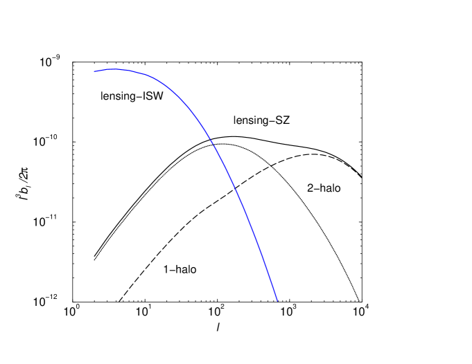
FIG. 1.: Power spectrum for the correlation of lensing angular deflections and the SZ effect, as calculated under the halo description. As shown, most of the contributions to the lensing-SZ correlation, as relevant for CMB, comes from large angular scale correlations between halos, denoted by the 2-halo term, and the mildly non-linear regime where contributions from individual halos are important (1-halo term). For reference, we also show the correlation power spectrum for lensing deflections and the integrated Sachs-Wolfe effect at late times.

II Calculational Method

The bispectrum $B_{l_{1}l_{2}l_{3}}$ is the spherical harmonic transform of the three-point correlation function just as the angular power spectrum $C_{\ell}$ is the transform of the two-point function. In terms of the multipole moments of the temperature fluctuation field $T(\hat{\bf n})$,

$$a_{lm}=\int d\hat{\bf n}T(\hat{\bf n})Y_{l}^{m}{}^{*}(\hat{\bf n})\,,$$ (1)

the two point correlation function is given by

$$C(\hat{\bf n},\hat{\bf m}) \equiv \langle T(\hat{\bf n})T(\hat{\bf m})\rangle$$ (2)

$$= \sum_{l_{1}m_{1}l_{2}m_{2}}\langle a_{l_{1}m_{1}}^{*}a_{l_{2}m_{2}}\rangle Y_{l_{1}}^{m_{1}}{}^{*}(\hat{\bf n})Y_{l_{2}}^{m_{2}}(\hat{\bf m})\,.$$ (3)

Under the assumption that the temperature field is statistically isotropic, the correlation is independent of $m$

$$\langle a_{l_{1}m_{1}}^{*}a_{l_{2}m_{2}}\rangle=\delta^{\rm D}_{l_{1}l_{2}}\delta^{\rm D}_{m_{1}m_{2}}C_{l_{1}}\,,$$ (4)

and is called the angular power spectrum. Likewise the three point correlation function is given by

$$B(\hat{\bf n},\hat{\bf m},\hat{\bf l}) \equiv \langle T(\hat{\bf n})T(\hat{\bf m})T(\hat{\bf l})\rangle$$ (5)

$$\equiv \sum\langle a_{l_{1}m_{1}}a_{l_{2}m_{2}}a_{l_{3}m_{3}}\rangle Y_{l_{1}}^{m_{1}}(\hat{\bf n})Y_{l_{2}}^{m_{2}}(\hat{\bf m})Y_{l_{3}}^{m_{3}}(\hat{\bf l})\,,$$ (6)

where the sum is over $(l_{1},m_{1}),(l_{2},m_{2}),(l_{3},m_{3})$. Statistical isotropy again allows us to express the correlation in terms of an $m$-independent function,

$$\langle a_{l_{1}m_{1}}a_{l_{2}m_{2}}a_{l_{3}m_{3}}\rangle=\left(\begin{array}[]{ccc}l_{1}&l_{2}&l_{3}\\ m_{1}&m_{2}&m_{3}\end{array}\right)B_{l_{1}l_{2}l_{3}}\,.$$ (9)

Here the quantity in parentheses is the Wigner-3$j$ symbol. The orthonormality relation for Wigner-3$j$ symbol implies

$$B_{l_{1}l_{2}l_{3}}=\sum_{m_{1}m_{2}m_{3}}\left(\begin{array}[]{ccc}l_{1}&l_{2}&l_{3}\\ m_{1}&m_{2}&m_{3}\end{array}\right)\langle a_{l_{1}m_{1}}a_{l_{2}m_{2}}a_{l_{3}m_{3}}\rangle\,.$$ (12)

The angular bispectrum, $B_{l_{1}l_{2}l_{3}}$, contains all the information available in the three-point correlation function. For example, the skewness, the pseudocollapsed three-point function of [12] and the equilateral configuration statistic of [8] can all be expressed as linear combinations of the bispectrum terms (see [14] for explicit expressions and [4] for an expression relating skewness in terms of the bispectrum).

The quantity of interest here is the correlation between squared temperature and temperature, instead of the usual temperature-temperature correlation. Following equation 3, we can write this power spectrum as

$$C^{2}(\hat{\bf n},\hat{\bf m}) \equiv \langle T^{2}(\hat{\bf n})T(\hat{\bf m})\rangle$$ (13)

$$= \sum_{l_{1}m_{1}l_{2}m_{2}}\langle a_{l_{1}m_{1}}^{2}a_{l_{2}m_{2}}^{*}\rangle Y_{l_{1}}^{m_{1}}(\hat{\bf n})Y_{l_{2}}^{m_{2}}{}^{*}(\hat{\bf m})\,.$$ (14)

Here, note that $a_{l_{1}m_{1}}^{2}$ is the multipole moments of the squared temperature field and not the square of the multipole moment of the temperature field, $(a_{l_{1}m_{1}})^{2}$. Through the expansion of the temperature

$$T(\hat{\bf n})=\sum a_{lm}Y_{l}^{m}(\hat{\bf n}),$$ (15)

we can write

$$a_{lm}^{2} = \int d\hat{\bf n}T^{2}(\hat{\bf n})Y_{l}^{m}{}^{*}(\hat{\bf n})$$ (16)

$$= \sum_{l_{1}m_{1}l_{2}m_{2}}a_{l_{1}m_{1}}a_{l_{2}m_{2}}\int d\hat{\bf n}Y_{l}^{m}{}^{*}(\hat{\bf n})Y_{l_{1}}^{m_{1}}(\hat{\bf n})Y_{l_{2}}^{m_{2}}(\hat{\bf n})\,.$$ (17)

We can now construct the power spectrum of squared temperature and temperature as

$$\langle a_{lm}^{2}a_{l^{\prime}m^{\prime}}^{*}\rangle=C_{l}^{2}\delta^{\rm D}_{ll^{\prime}}\delta^{\rm D}_{mm^{\prime}}$$ (18)

$$= \sum_{l_{1}m_{1}l_{2}m_{2}}\langle a_{l_{1}m_{1}}a_{l_{2}m_{2}}a_{l^{\prime}m^{\prime}}^{*}\rangle\int d\hat{\bf n}Y_{l}^{m}{}^{*}(\hat{\bf n})Y_{l_{1}}^{m_{1}}(\hat{\bf n})Y_{l_{2}}^{m_{2}}(\hat{\bf n})\,.$$ (19)

Using the Gaunt integral

$$\int d\hat{\bf n}Y_{l_{1}}^{m_{1}}Y_{l_{2}}^{m_{2}}Y_{l_{3}}^{m_{3}} = \sqrt{(2l_{1}+1)(2l_{2}+1)(2l_{3}+1)\over 4\pi}$$ (25)

$$\times\left(\begin{array}[]{ccc}l_{1}&l_{2}&l_{3}\\ 0&0&0\end{array}\right)\left(\begin{array}[]{ccc}l_{1}&l_{2}&l_{3}\\ m_{1}&m_{2}&m_{3}\end{array}\right)\,,$$

and introducing the bispectrum from equation 9, we can write the angular power spectrum of squared temperature and temperature as

$$C_{l}^{2}=\sum_{l_{1}l_{2}}B_{l_{1}l_{2}l}w_{l_{1},l_{2}}\left(\begin{array}[]{ccc}l_{1}&l_{2}&l\\ 0&0&0\end{array}\right)\sqrt{(2l_{1}+1)(2l_{2}+1)\over 4\pi(2l+1)}\,.$$ (27)

In simplifying, we have made use of the fact that

$$\sum_{m_{1}m_{2}}\left(\begin{array}[]{ccc}l_{1}&l_{2}&l\\ m_{1}&m_{2}&m\end{array}\right)\left(\begin{array}[]{ccc}l_{1}&l_{2}&l^{\prime}\\ m_{1}&m_{2}&m^{\prime}\end{array}\right)=\frac{\delta^{\rm D}_{ll^{\prime}}\delta^{\rm D}_{mm^{\prime}}}{2l+1}\,.$$ (28)

Equation 27, is the expression of interest here. This relates the angular bispectrum to the angular power spectrum of squared temperature and temperature. In taking a general approach, we have introduced a filter, or window, function in Fourier space of $w_{l_{1},l_{2}}$. We will later discuss detailed forms for the appropriate filter functions later.

Since the bispectrum is defined by a triangle in multipole space with lengths of sides $(l,l_{1},l_{2})$, the $C_{l}^{2}$ power spectrum essentially captures information, through a summation, associated with all triangular configurations with one of the sides of length $l$. If apriori known that certain triangular configurations contribute to the bispectrum significantly, such as flattened triangles in the case of certain secondary correlations (see, [7]), one can compute this sum by only restricting the multipoles of interest. This is essentially what can be achieved with the introduction of an appropriate window, or a filter, function to the squared temperature field. Though the expression for the angular power spectrum involves a bispectrum, the experimental measurement is straightforward: one construct the power spectrum by squaring the temperature field, in real space, and using the Fourier transforms of squared temperature values and the temperature field, with any filtering functions, when necessary.

We will now discuss the measurement of the power spectrum using Planck data for the non-Gaussian signal involved through the correlation between lensing angular deflections and the SZ effect. This bispectrum has the high cumulative signal-to-noise out of all other possible bispectra involving secondary effects and CMB temperature [7]. For the illustration of our results we use the currently favored $\Lambda$CDM cosmological model. The parameters for this model are $\Omega_{c}=0.30$, $\Omega_{b}=0.05$, $\Omega_{\Lambda}=0.65$, $h=0.65$, $Y_{p}=0.24$, $n=1$, COBE normalization $\delta_{H}=4.2\times 10^{-5}$ [17]. This model has mass fluctuations on the $8h$ Mpc^-1 scale in accord with the abundance of galaxy clusters $\sigma_{8}=0.86$ [23].

III CMB²-SZ power spectrum

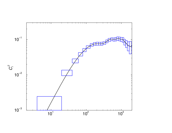
FIG. 2.: The angular power spectrum of CMB²-SZ due to the correlation of SZ effect and gravitational lensing in CMB. The band power errors are for the Planck mission using the noise calculation for multifrequency separation of SZ and CMB effect from Planck data.

FIG. 3.: Optimal filter function for the CMB²-SZ power spectrum, as a function of $l_{1}$ and $l_{2}$. In left, the filter is when $l=100$ and right is when $l=2000$ corresponding to large and small angular scales respectively. The optimal filter behaves such that it removes excess noise at multipoles less than $\sim$ 1500 and extracts sensitivity of lensing in the damping tail of the power spectrum.

We refer the reader to [7] for a full derivation of the bispectra due to correlations between lensing angular deflections in CMB and secondary effects due to large scale structure. Following these derivations, we can write the bispectrum as

$$B_{l_{1},l_{2},l}=-\left(\begin{array}[]{ccc}l_{1}&l_{2}&l\\ 0&0&0\end{array}\right)\sqrt{\frac{(2l_{1}+1)(2l_{2}+1)(2l+1)}{4\pi}}$$ (31)

$$\times \left[f_{l_{2},l_{1},l}C_{l_{1}}^{\rm CMB}b_{l}+{\rm Perm.}\right]\,,$$ (32)

where

$$f_{l_{a},l_{b},l_{c}}=\left[\frac{l_{a}(l_{a}+1)-l_{b}(l_{b}+1)-l_{c}(l_{c}+1)}{2}\right]\,,$$ (34)

and $b_{l}$ is the cross-correlation power spectrum involved with lensing angular deflections and a secondary source of anisotropies that trace the large scale structure and effectively correlates with lensing potentials (e.g., integrated Sachs-Wolfe effect [15], linear Doppler effect, SZ effect). Here, we consider the case of SZ since, as discussed in [7], the correlation between lensing and other two effects does not lead to a bispectrum with significant signal-to-noise.

If the two maps involved with the construction of the squared temperature-temperature power spectrum is the same (e.g., CMB alone), then the permutation in equation LABEL:eqn:cmbbi leads to a total of 6 terms in the ordering of $l_{1}$, $l_{2}$ and $l$. When the bispectrum is measured with two independent maps, e.g., CMB and SZ through frequency cleaning, the permutation in equation LABEL:eqn:cmbbi involves an additional term with the replacement of $l_{1}$ by $l_{2}$.

We now primarily consider the case of two independent maps with Planck, and thus, we can write the CMB²-SZ power spectrum as

$$C_{l}^{2} = b_{l}\sum_{l_{1}l_{2}}\left(\begin{array}[]{ccc}l_{1}&l_{2}&l\\ 0&0&0\end{array}\right)^{2}{(2l_{1}+1)(2l_{2}+1)\over 4\pi}w_{l_{1},l_{2}}^{2}$$ (37)

$$\times \left[C_{l_{1}}^{\rm CMB}f_{l_{2},l_{1},l}+C_{l_{2}}^{\rm CMB}f_{l_{1},l_{2},l}\right]\,.$$ (38)

Here, $C_{l}^{\rm CMB}$ is the unlensed primary CMB contribution.

The proposed use of the CMB²-SZ power spectrum is essentially following. One can directly measure $C_{l}^{2}$ in the CMB and SZ data and since information related to $C_{l}^{\rm CMB}$ also directly comes from data, one can construct the quantity $b_{l}$ which is directly proportional to $C_{l}^{2}$. As written in equation 38, in the case relevant to the CMB²-SZ power spectrum, the cross-correlation between lensing deflections and the SZ effect

$$b_{l}=\int dr\frac{W^{\rm SZ}(r)W^{\rm len}(k,r)|_{k=l/d_{A}}}{d_{A}^{2}}P_{\Pi\delta}({l\over d_{A}};r)\,.$$ (39)

Here, we have utilized the Limber approximation [24] by setting $k=l/d_{A}$, $P_{\Pi\delta}$ is the pressure-dark matter cross power spectrum, $r$ is the comoving radial distance and $d_{A}$ is the comoving angular diameter distance. The window functions for the SZ and lensing deflections are

$$W^{\rm SZ}(r)=g(x)\frac{k_{B}\sigma_{T}\bar{n}_{e}}{a(r)^{2}m_{e}c^{2}}$$ (40)

and

$$W^{\rm len}(k,r)=-3\frac{\Omega_{m}}{a(r)}\left(\frac{H_{0}}{k}\right)^{2}\frac{d_{A}(r_{s}-r)}{d_{A}(r)d_{A}(r_{s})}\,,$$ (41)

respectively. In Eq. 40, $\bar{n}_{e}$ is the mean density of electrons today, $\sigma_{T}$ is the Thomson cross-section and $g(x)=x\coth(x/2)-4$ with $x=h\nu/k_{B}T_{\rm CMB}$ is the spectral shape of the SZ effect. At Rayleigh-Jeans part of the CMB, $g(x)=-2$. As discussed in [4], an experiment such as Planck with observations over a wide range of frequencies can separate out SZ contributions based on the spectral signature, $g(x)$ relative to primary CMB and other contributors. For this paper, we will consider Planck in estimating signal-to-noise and will use the noise power spectra calculated in [4] for the Planck SZ and CMB maps.

In order to assess how well Planck CMB and SZ maps can be used for the purpose of constructing $b_{l}$, we need to consider an estimate for it, as well as, estimates for $C_{l}^{\rm CMB}$ and $C_{l}^{\rm SZ}$; The latter is required when estimating the signal-to-noise for possible detections. We use CMBFAST of [28] and compue $b_{l}$ and $C_{l}^{\rm CMB}$ analytically using a semi-analytical description of pressure fluctuations in the large scale structure involving the halo approach [18]. To calculate $b_{l}$ we need the pressure-dark matter cross-power spectrum while $C_{l}^{\rm SZ}$ depends on the pressure-pressure power spectrum. The power spectra are introduced and discussed in detail in [9, 10] and we refer the reader to these two papers for for further details on this approach. The basic assumption of the halo model is that large scale structure dark matter distribution can be viewed as a collection of dark matter halos with a mass function following Press-Schechter [19] mass function or variants and a dark matter distribution in each halo following NFW profile of [20] or other descriptions. The halos are biased relative to the linear density field following the description of [21]. With clustering of dark matter described through such an approach, any other physical property of the large scale structure can be easily described through the relation between that property and dark matter. For example, in the case of pressure, we can gas distribution in each halos follow hydrostatic equillibrium with dark matter. As discussed in [10], such an approach through the halo model provides a reliable semi-analytic approach to model non-linear large scale structure clustering and its predictions, in the case of pressure as relevant for the SZ effect and lensing-SZ correlations, are consistent with numerical simulations (e.g., [22]).

In figure 1, we show the correlation between lensing deflections and SZ effect. The contributions are broken to singlem 1-halo, and 2-halo term involving correlations between and within halos. As shown, for multipoles of interest, most of the correlation comes from the 2-halo term involving large scale correlations between halos, though at multipoles $\sim$ few hundred, the contribution from single halo term cannot be ignored. This is the mildly non-linear regime where contributions from large scale correlations between halos and the halo profiles become important.

Following the correlation between lensing and SZ shown in figure 1, in figure 2, we show the $C_{l}^{2}$ power spectrum due to the relevant bispectrum. We now discuss the calculation of errors shown in figure 2.

A Signal to Noise

To establish the signal-to-noise for the detection of the lensing-SZ bispectrum through the squared temperature-temperature power spectrum, we calculate the covariance associated with the proposed statistic following [10]. Here, we assume that the squared temperature and temperature power spectrum will be measured with two maps involving CMB and SZ with squared temperature measurement from the CMB map and a single temperature measurement from SZ. We can write the error on each of the power spectrum measurements associated with the proposed statistic as

$$\Delta C_{l}^{2}=\sqrt{\frac{1}{f_{\rm sky}(2l+1)}}\left[\left(C_{l}^{2}\right)^{2}+C_{l,tot}^{2\rm CMB}C_{l,tot}^{\rm SZ}\right]^{1/2}\,,$$ (42)

while the total signal-to-noise is

$$\frac{S}{N}=\left[f_{\rm sky}\sum_{l}(2l+1)\frac{\left(C_{l}^{2}\right)^{2}}{\left(C_{l}^{2}\right)^{2}+C_{l,tot}^{2\rm CMB}C_{l,tot}^{\rm SZ}}\right]^{1/2}\,,$$ (43)

with the fraction of sky covered by $f_{\rm sky}$.

Here, the propose squared temperature and temperature angular power spectrum is $C_{l}^{2}$ and $C_{l,tot}^{2\rm CMB}$ is the squared temperature power spectrum in CMB data alone,

$$C_{l,tot}^{2\rm CMB}=$$ (44)

$$\sum_{l_{1}l_{2}}2C_{l_{1},tot}^{\rm CMB}C_{l_{2},tot}^{\rm CMB}w_{l_{1},l_{2}}^{2}\left(\begin{array}[]{ccc}l_{1}&l_{2}&l_{3}\\ 0&0&0\end{array}\right)^{2}\frac{(2l_{1}+1)(2l_{2}+1)}{4\pi}\,.$$ (47)

In calculating the noise, following [25], we also include relevant detector and frequency separation noise — for the SZ map — by introducing $C_{l,tot}^{\rm CMB}=C_{l}^{\rm CMB}+C_{l}^{\rm S}+C_{l}^{\rm N}$, with $S$ denoting other secondary contributors in the CMB map (e.g., lensing) and $N$ is the noise contribution. There is an additional term here involving the CMB trispectrum which leads to the covariance between multipoles. We ignore it here given that there is no significant non-Gaussian component to the primary anisotropies especially in the adiabatic CDM models [6], which are more consistent with current observations of large scale structure and CMB. The next important contribution to the covariance of CMB comes from secondary effects with a thermal spectrum. As discussed in Hu [11], gravitational lensing of CMB, which is the most important secondary effect that leads to non-Gaussian correlations, does not produce a significant covariance out to $l$ of 2000 as relevant for the Planck mission. Thus, we ignore the presence of a non-Gaussian trispectrum in our variance estimates and only consider Gaussian contributions. At further small angular scales, in addition to lensing, other secondary effects with a CMB thermal spectral signature, such as kinetic SZ effect, can produce a trispectrum in CMB temperature data (see, [10]).

Note that since we consider frequency separated maps, there is no trispectrum contribution to the covariance of the proposed statistic from the SZ effect and contribution to the variance comes only from the SZ power spectrum $C_{l}^{\rm SZ}$. We calculated this power spectrum again using the halo model following [10]. If the measurement is to be done in a map which is not frequency cleaned with components separated out, then the trispectrum involved with SZ will also contribute to the covariance.

B Filter functions

Here, we consider two possibilities for the filtering of unnecessary noise in the $T^{2}$ map. A straightforward filter is to essentially remove the excess low multipole noise and we achieve this by choosing

$\displaystyle\mbox{$w_{l_{1},l_{2}}$}=\left\{\begin{array}[]{ll}1&\mbox{$l_{1},l_{2}>l_{\rm cut}$}\\ 0&\mbox{$l_{1},l_{2}<l_{\rm cut}$}\end{array}\right.$

where we set the $l_{\rm cut}$ to be 1000. Note that in the case of Planck, instrumental noise degrades the information beyond a $l$ of 2000.

FIG. 4.: The cumulative signal-to-noise for the detection of temperature²-temperature power spectra in Planck data. The top figure is using the filtering scheme where we remove excess noise at multipoles $l_{1}$ and $l_{2}$ of less than 1000. The shown curves are for with no SZ separation (dotted), with SZ separation (solid), and perfect SZ separation with no noise contribution to both SZ and CMB maps (dashed). In the realistic case of SZ separation, the total cumulative signal-to-noise is of order $\sim$ 20. The bottom panel compares the signal-to-noise for Planck with no filtering (dotted line) and optimal filtering (long dashed line). Optimal filtering leads to a cumulative signal-to-noise of $\sim$ 70.

Additionally, we consider an optimal filtering scheme which maximizes the $(S/N)^{2}$ in equation 43. Analytically, this is equivalent to taking the derivative of the expression in equation 43 with respect to $w_{l_{1},l_{2}}$ and solving for the value which maximizes the signal-to-noise. We found this to be when

$$w_{l_{1},l_{2}}=\frac{\left[C_{l_{1}}^{\rm CMB}f_{l_{2},l_{1},l}+C_{l_{2}}^{\rm CMB}f_{l_{1},l_{2},l}\right]}{2C_{l,tot}^{\rm CMB}C_{l_{2},tot}^{\rm CMB}}\,,$$ (48)

with an appropriate normalization such that $\sum_{l_{1}l_{2}}w_{l_{1},l_{2}}=1$. This optimal filter is equivalent to the one introduced by Hu [11] for the estimator of the deflection angles in CMB using a quadratic statistic. Note that the optimal filter is independent of the correlation power between lensing deflections and the SZ effect, however, depends on the details of mode coupling associated with lensing in CMB through the $f$ terms. One can easily construct the filter through apriori knowledge on the CMB power spectrum and noise properties.

When the optimal filter is applied to the squared temperature map, $C_{l,tot}^{2\rm CMB}=C_{l}^{2}$, and this leads to a simplified expression for the signal-to-noise of the CMB²-SZ power spectrum

$$\left(\frac{S}{N}\right)^{2} \approx f_{\rm sky}\sum_{ll_{1}l_{2}}\left(\begin{array}[]{ccc}l_{1}&l_{2}&l\\ 0&0&0\end{array}\right)^{2}{(2l_{1}+1)(2l_{2}+1)\over 4\pi}$$ (51)

$$\times \frac{\left[C_{l_{1}}^{\rm CMB}f_{l_{2},l_{1},l}+C_{l_{2}}^{\rm CMB}f_{l_{1},l_{2},l}\right]^{2}b_{l}^{2}}{2C_{l_{1},tot}^{\rm CMB}C_{l_{2},tot}^{\rm CMB}C_{l,tot}^{\rm SZ}}$$ (52)

$$= f_{\rm sky}\sum_{ll_{1}l_{2}}\frac{B^{2}_{l_{1}l_{2}l}}{2C_{l_{1},tot}^{\rm CMB}C_{l_{2},tot}^{\rm CMB}C_{l,tot}^{\rm SZ}}\,.$$ (53)

As written above, the total signal-to-noise is now equal to exactly the total amount present in the full bispectrum formed by correlations between gravitational lensing deflections in CMB and the SZ effect (see, [7]). Thus, the optimal filter allows one to capture, at the two point level through basically a power spectrum, all information contained within the bispectrum at the three point level; this happens with no loss in signal-to-noise. The temperature-gradient divergence statistic introduced by [11] allows this to be carried out directly; with appropriate optimal filtering suggested above, this is equivalent to the CMB²-SZ approached outlined here.

In figure. 3, we show the surface of the optimal filter as a function of $l_{1}$ and $l_{2}$ when $l_{3}=100$ and 2000, respectively. As shown, the optimal filter behaves such that one only used information in multipole range with $l_{1}$ and $l_{2}$ $\gtrsim 1500$. This behavior is the reason why that a simple filter with the behavior of a step-function in $l_{1}$ and $l_{2}$ essentially allows us to capture some of the information present in the bispectrum. The detailed behavior of the optimal filter function, especially information related to lensing present in the peaks and valleys of the CMB power spectrum, however, limits the information that can be captured by a simple filter. The optimal filter behaves such that it effectively extracts all information related to lensing from the damping tail of the CMB power spectrum.

IV Discussion

In figure 1, we show the correlation between SZ effect and lensing angular deflections. The cross angular power spectrum is weighted by a factor of $l^{3}$ to highlight the multipole range which is important for the CMB bispectrum due to gravitational lensing-secondary correlations. For comparison, in the same plot, we show the correlation power between lensing deflections and the integrated Sachs-Wolfe effect (ISW; [15]) at late times. We refer the reader to Cooray & Hu [7] for a detailed discussion of the bispectra produced through correlations between gravitational lensing angular deflections and secondary effects. In the case of the lensing-SZ, note that we have updated the calculations presented therein using a detailed description of large scale structure pressure fluctuations instead of the assumption that pressure traces dark matter (see, [9, 10] for a discussion on the computation of statistics related to large scale structure pressure); The assumption of pressure traces dark matter, in general, leads to an slight overestimate of the correlation between lensing and SZ.

The lensing-SZ correlation behaves such contributions relavant for the CMB bispectrum, at multipoles less than 100, comes from interhalo large scale correlations, which we defined as the 2-halo term in [9, 10], involving the linear density field. The mildly non-linear regime, at multipoles around few hundred, is described through the combination of large scale correlations and the interhalo correlations through the profiles denoted by the 1-halo term. This behavior is consistent with the fact that angular deflections in CMB is a large scale phenomena with an angular coherence of the deflection angle of $\sim$ 10 degrees (see, [13]). Though lensing windown function peaks at a redshift of $\sim$ 3, at half the angular diameter distance to last scattering, the non-linear contributions to the lensing-SZ correlations comes primarily from the SZ effect which has a window function that effectively peaks at very low redshifts; overall, contributions to the lensing-SZ correlations comes over a wide-range of redshifts and the low redshift behavior of the SZ effect makes the contribution from the 1-halo term important at small angular scales.

Note that most of the contributions come at multipoles greater than few hundred, with a tail continues to multipoles of thousands. Since CMB itself dominates low multipoles, its contribution to the variance is more important at multipoles less than $\sim$ 1000. This is the same reason why the lensing-ISW effect, even with a significantly higher correlation at very large angular scales, leads to considerably smaller signal-to-noise for the bispectrum and thus, to the squared temperature-temperature power spectrum.

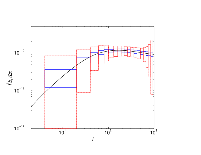
FIG. 5.: Power spectrum for the correlation of lensing angular deflections and the SZ effect, as calculated under the halo description. The band power errors are from the measurement of CMB²-SZ power spectrum in Planck with frequency cleaned CMB and SZ maps with a filtering scheme where noise is removed at multipoles less than 1000 (dotted) and using the optimal filtering (solid). The experimental measurement of the SZ-lensing deflections cross power spectrum is important for the understanding of relation between large scale pressure and dark matter fluctuations.

In figure 2, we show the angular power spectrum of CMB²-SZ power spectrum using the halo model description of $b_{l}$. We computed the power spectrum band errors by using the optimal filtering scheme discussed in § III B and shown in figure 3 and using equation 42 to compute errors. Here, we consider the Planck measurement of the SZ effect and use the variance power spectrum calculated in [4]. We also include the relevant beam/detector noise in the CMB map. For secondary contributors to the noise, we include contribution from lensing and non-linear kinetic SZ following [13] and [10]. The effect of the optimal filter is to remove the noise associated with low multipoles primarily from the intrinsic CMB anisotropies, while extracting information related to lensing associated with peaks and valleys in the CMB power spectrum as well as small scall information coming from the modification of a CMB gradient on the sky. As shown, Planck derived CMB and SZ maps can be clearly used to detect the CMB²-SZ non-Gaussian bispectrum due to lensing at the two-point level.

In figure 4, we show the cumulative signal-to-noise associated with this detection. Here, we consider both the optimal filtering as well as our crude filter where we removed all information at multipoles less than 1000. In the top panel, we consider this latter scenario. Using the frequency cleaned maps, the signal-to-noise ranges up to $\sim$ 20, while with no frequency cleaning we only find a value around 6. If Planck were to allow perfect separation of SZ and CMB and with no noise contributions to both SZ and CMB maps, and with only cosmic variance, one finds a total signal-to-noise of $\sim$ 60. This increase in signal-to-noise primarily comes from multipoles greater than 1000 and is due to the decrease in the noise associated with the SZ map. Clearly, improving the separation of SZ from CMB and decreasing the associated noise can lead to a significantly better detection of the lensing-SZ correlation through the CMB²-SZ power spectrum.

In the bottom panel of figure 4, we compare cumulative signal-to-noise with no filtering, optimal filtering and with our simple noise removal at $l\lesssim 1000$ and $l\lesssim 1500$. Here again, we consider the Planck CMB and SZ maps. With no filtering, cumulative signal-to-noise is of order $\sim$ 3, while with optimal filtering, one obtains a total signal-to-noise of $\sim$ 70. With the simple noise removal at $l$ of 1000, one has only gained a factor of $\sim$ 6, while this is still a factor of $\sim$ 3.5 less than optimal case. As shown in figure 3, when large scales are considered, the filter removes excess noise out to $l_{1},l_{2}$ of 1500. Thus, we introduced simple noise removal out to $l$ of 1500. As shown in figure 4 (bottom panel) with a dot-dashed line, even though there is an increase in signal-to-noise at low $l$ values, consistent with the behavior of the optimal filter function, one finds less cumulative signal-to-noise at small angular scales. Such differences are primarily due to the detailed behavior of the optimal filter. With a simple filter, no information is obtained from multipoles that is associated with peaks and valleys of the CMB power spectrum, while related information is contained within the optimal filter. Though one can obtain relatively modest measurement of the CMB²-SZ power spectrum through crude filtering, an optimal filter, such as the one suggested here, is highly recommended to exploit the full potential of the measurable signal.

In addition to the CMB²-SZ power spectrum, or a constructing through the temperature-gradient divergence statistics of [11], an alternative technique to construct the lensing-SZ correlation involves the gradient statistic of [26]. This technique utilizes gradient maps and an analysis similar to polarization to construct a map that is directly proportional to weak lensing convergence. With such a statistic, and following the procedure in [26, 27], we find a cumulative signal-to-noise of $\sim$ 35, which is better than the simple filter but roughly a factor of 2 worse than the optimal filter considered here.

Given that the proposed statistic involving CMB²-SZ power spectrum is directly proportional to the cross-power spectrum between lensing angular deflections and the SZ effect, our error estimates on $C_{l}^{2}$ can be converted to those of $b_{l}$. In figure 5, we show the band power errors on $b_{l}$ using the Planck estimates for errors on CMB²-SZ power spectrum using the simple filter (dashed line) and the optimal filter (solid lines). As shown, Planck allows a clear detection of the cross-correlation between SZ and lensing deflections; the detection is very clear with the optimal filter. The experimental measurement of this correlation power spectrum is preferred since it contains important cosmological and astrophysical information related to large scale fluctuations of pressure and dark matter. When combined with SZ-SZ power spectrum and the lensing-lensing power spectrum either from large scale structure weak lensing or CMB directly, this lensing-SZ power spectrum will provide us knowledge on the correlation between pressure and dark matter. The proposed squared temperature-temperature statistic involving Planck CMB and SZ maps, with appropriate filtering, is clearly one of the few ways to obtain this information.

- [1]
- [2] L. Knox, Phys. Rev. D, 52 4307 (1995); G. Jungman, M. Kamionkowski, A. Kosowsky and D.N. Spergel, Phys. Rev. D, 54 1332 (1995); J.R. Bond, G. Efstathiou and M. Tegmark, MNRAS, 291 L33 (1997); M. Zaldarriaga, D.N. Spergel and U. Seljak, Astrophys. J., 488 1 (1997); D.J. Eisenstein, W. Hu and M. Tegmark, Astrophys. J., 518 2 (1999)
- [3] R. A. Sunyaev and Ya. B. Zel’dovich, MNRAS, 190, 413 (1980)
- [4] A. Cooray, W. Hu and M. Tegmark, Astrophys. J., 540, 1 (2000)
- [5] L. Knox, A. Cooray, D. Eisenstein and Z. Haiman, Astrophys. J., 550, 7 (2001).
- [6] E. Komatsu and D. N. Spergel, preprint, astro-ph/0005036; L. Wang and M. Kamionkowski, Phys. Rev. D, 61, 063504 (1999); A. Gangui and J. Martin, MNRAS, 313, 323 (2000); X. Luo and D. N. Schramm, Phys. Rev. Lett., 71, 1124 (1994); X. Luo Astrophys. J., 427, 71 (1994); T. Falk, R. Rangarajan and M. Frednicki, Astrophys. J. Lett.403, L1 (1993);
- [7] A. Cooray and W. Hu, Astrophys. J., 534, 533 (2000); D. M. Goldberg and D. N. Spergel, Phys. Rev. D, 59, 103002 (1999); D. N. Spergel and D. M. Goldberg Phys. Rev. D, 59, 103001 (1999)
- [8] P. G. Ferreira, J. Magueijo and K. M. Gorksi, Astrophys. J., 503, 1 (1998); for updates, see also, J. Pando, D. Vallas-Gabaud D. and L. Fang, Phys. Rev. Lett., 79, 1611 (1998); A. J. Banday, S. Zaroubi, S. and K. M. Gorski, Astrophys. J.in press (astro-ph/9908070); B. Bromley and M. Tegmark, Astrophys. J. Lett., 524, L79 (1999)
- [9] A. Cooray, Phys. Rev. D, 62, 19452 (2000).
- [10] A. Cooray, Phys. Rev. D., submitted (astro-ph/0105063); also, A. Cooray, 2001, Ph.D. thesis, University of Chicago, Chicago (2001); available from the U. of Chicago Crear Science Library or from the author.
- [11] W. Hu, 2001, Phys. Rev. D. submitted (astro-ph/0105117).
- [12] G. Hinshaw, A. J. Banday, C. L. Bennett, K. M. Gorski and A. Kogut, Astrophys. J., 446, 67 (1995)
- [13] W. Hu, A. Cooray, Phys. Rev. D, 63, 023504 (2000).
- [14] A. Gangui, F. Lucchin, S. Matarrese and S. Mollerach, Astrophys. J., 430, 447 (1994)
- [15] R. K. Sachs and A. M. Wolfe, Astrophys. J., 147, 73 (1967)
- [16] D. J. Eisenstein and W. Hu, Astrophys. J., 511, 5 (1999)
- [17] E. F. Bunn and M. White, Astrophys. J., 480, 6 (1997)
- [18] R. J. Scherrer and E. Bertschinger, Astrophys. J., 381, 349 (1991); R. K. Sheth and B. Jain, MNRAS, 285, 231 (1997); U. Seljak, MNRAS, 318, 203 (2000); C.-P. Ma and J. N. Fry, Astrophys. J., 543, 503 (2000); A. Cooray and W. Hu, Astrophys. J., 548, 7 (2001); R. Scoccimarro, R. Sheth, L. Hui and B. Jain, Astrophys. J., 546, 20 (2001)
- [19] W. H. Press and P. Schechter, Astrophys. J., 187, 425 (1974); see, also, R. K. Sheth and B. Tormen, MNRAS, 308, 119 (1999).
- [20] J. Navarro, C. Frenk and S. D. M. White, Astrophys. J., 462, 563 (1996).
- [21] H. J. Mo, Y. P. Jing and S. D. M. White, MNRAS, 284, 189 (1997); H. J. Mo and S. D. M. White, MNRAS, 282, 347 (1996).
- [22] A. Refregier and R. Teyssier, Phys. Rev. D, submitted, astro-ph/0012086 (2001).
- [23] P. T. P. Viana and A. R. Liddle MNRAS, 303, 535 (1999)
- [24] D. Limber, Astrophys. J., 119, 655 (1954)
- [25] L. Knox, Phys. Rev. D, 48, 3502 (1995)
- [26] M. Zaldarriaga and U. Seljak, Phys. Rev. D, 59, 123507 (1999)
- [27] H. V. Peiris and D. N. Spergel, Astrophys. J., in press (astro-ph/001393)
- [28] U. Seljak and M. Zaldarriaga, Astrophys. J., 469, 437 (1996)