Order and chaos in the local disc stellar kinematics induced by the Galactic bar

The Galactic bar causes a characteristic splitting of the disc phase space into regular and chaotic orbit regions which is shown to play an important role in shaping the stellar velocity distribution in the Solar neighbourhood. A detailed orbital analysis within an analytical 2D rotating barred potential reveals that this splitting is mainly dictated by the value of the Hamiltonian $H$ and the bar induced resonances. In the $u-v$ velocity plane at fixed space position, the contours of constant $H$ are circles centred on the local solid rotation velocity of the bar frame and of radius increasing with $H$. For reasonable bar strengths, the contour $H=H_{12}$ corresponding to the effective potential at the Lagrangian points $L_{1/2}$ marks the average transition from regular to chaotic motion, with the majority of orbits being chaotic at $H>H_{12}$. On top of this, the resonances generate an alternation of regular and chaotic orbit arcs opened towards lower angular momentum and asymmetric in $u$ for space positions away from the principal axes of the bar. Test particle simulations of exponential discs in the same potential and a more realistic high-resolution 3D $N$-body simulation reveal how the decoupled evolution of the distribution function in the two kind of regions and the process of chaotic mixing lead to overdensities in the $H\ga H_{12}$ chaotic part of the disc velocity distributions outside corotation. In particular, for realistic space positions of the Sun near or slightly beyond the outer Lindblad resonance and if $u$ is defined positive towards the anti-centre, the eccentric quasi-periodic orbits trapped around the stable $x_{1}(1)$ orbits – i.e. the bar-aligned closed orbits which asymptotically become circular at larger distances – produce a broad $u\la 0$ regular arc in velocity space extending within the $H>H_{12}$ zone, whereas the corresponding $u\ga 0$ region appears as an overdensity of chaotic orbits forced to avoid that arc. This chaotic overdensity provides an original interpretation, distinct from the anti-bar elongated quasi-periodic orbit interpretation proposed by Dehnen (D5 (2000)), for the prominent stream of high asymmetric drift and predominantly outward moving stars clearly emerging from the Hipparcos data. However, the most appropriate interpretation for this stream remains uncertain. The effects of spiral arms and of molecular clouds are also briefly discussed within this context.

1 Introduction

The kinematics of disc stars in the Solar neighbourhood displays several long known properties, such as the increase of velocity dispersion with age, the tendency of young stars to appear in moving groups or streams, and the classical vertex deviation affecting stars with asymmetric drift down to $\sim 25$ km s^-1 relative to the Sun and mainly owing to the Hyades and Sirius streams. Disc heating is traditionally attributed to the diffusion of stars by transient spiral arms or by massive compact objects like molecular clouds, the streams to dissolving ensembles of stars born at the same place, and the vertex deviation to local gravitational perturbations like spiral arms or local departures from a steady state.

Beside these properties, the local disc velocity distribution also betrays a broad stream of low angular momentum and mainly outward moving stars with a mean heliocentric asymmetric drift $s\approx 45$ km s^-1, i.e. typical of the thick disk (Gilmore et al. GWK (1989)), which hereafter will be referred to as the “Hercules” stream, according to the comoving Eggen group $\zeta$ Herculis (Skuljan et al. SHC (1999)). The mean outward motion of stars with high asymmetric drift, also known as the “$u$-anomaly” and seen up to over $s=100$ km s^-1 in metal rich samples (Raboud et al. RGMFS (1998)) and in Mira variables with period between $145$ and $200$ days (Feast & Whitelock FW (2000)), is already apparent in early stellar kinematical samples (Eggen E (1966); Woolley et al. WEPP (1970)) and was recognised long ago by Mayor (M (1972)), but the clearest evidence for the Hercules stream comes from the Hipparcos proper motions combined with (Fig. 1) or without (Dehnen D1 (1998)) available radial velocities. This stream is very likely to have a dynamical origin because its stars are older than $\sim 2$ Gyr (Caloi et al. CCD (1999)) and present a wide range of metallicities (Raboud et al. RGMFS (1998)).

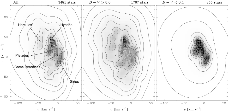
Figure 1: Heliocentric velocity distribution in the $u-v$ plane of all the Hipparcos single stars with $\sigma(\pi)/\pi<0.1$, $d<100$ pc and radial velocities in the Hipparcos Input Catalogue (left) and of the sub-samples with $B-V>0.6$ (middle) and $B-V<0.4$ (right). For the sake of comparison, the contours are as in Dehnen (D1 (1998)), containing $2$, $6$, $12$, $21$, $33$, $50$, $68$, $80$, $90$, $95$, $99$ and $99.9$ percent of all stars. The diagram for the full sample is exactly the same as in Fux (F3 (2000)), except for a different labelling of the contours.

The existence of the Hercules stream is most probably related to the influence of the Galactic bar. It is now indeed widely accepted that the Milky Way is a barred galaxy, as are the majority of disc galaxies. Evidence for the bar comes from longitudinal asymmetry in the bulge surface photometry (e.g. Blitz & Spergel BS (1991); Binney et al. BGS (1997)), star counts (e.g. Nakada et al. NDH (1991); Nikolaev & Weinberg NW (1997); Stanek et al. SU (1997)), interpretation of the observed gas kinematics in the central few kpc (Binney et al. BGSBU (1991); Englmaier & Gerhard EG (1999); Fux F2 (1999); Weiner & Sellwood WS (1999)), large microlensing optical depths towards the Galactic bulge (Paczynski et al. PSU (1994); Kuijken KK (1997); Gyuk GY (1999); Alcock et al. AAA (2000)) and possibly inner stellar kinematics (Sevenster et al. SSVF (1999); see also Gerhard OG (1999) for a recent review). Although still not very well constrained, the most quoted values for the main bar parameters are an in-plane inclination angle with respect to the Galactic centre direction $\varphi\approx 15^{\circ}-45^{\circ}$, with the near side of the bar in the first Galactic quadrant, and a corotation radius $R_{\hbox{\tiny CR}}\approx 3.5-5$ kpc.

Barred $N$-body models of the Milky Way produce a mean outward motion of disc particles at realistic positions of the Sun relative to the bar (Fux et al. FMP (1995); Raboud et al. RGMFS (1998)), but the precise bar induced dynamical process leading to the observed kinematical properties of the Hercules stream is still a matter of debate. Dehnen (1999b , D5 (2000) – hereafter D2000) relates this stream and the main mode of high angular momentum stars in the observed velocity distribution to the coexistence near the outer Lindblad resonance (OLR) of two distinct types of periodic orbits replacing the circular orbit close to the OLR in a rotating barred potential, i.e. the same idea introduced by Kalnajs (K (1991)) to explain the Hyades and Sirius streams. Linear theory indeed predicts that the orientation of orbits closing in the bar rotating frame changes across the main resonances associated with the bar (Binney & Tremaine BT (1987)). In particular, periodic orbits outside and inside the OLR radius are respectively elongated along the major and minor axis of the bar, and both types of orbits, as well as the quasi-periodic orbits trapped around these orbits, can overlap in space near the OLR. According to D2000, the Hercules stream and the main velocity mode, respectively “OLR” and “LSR” mode in his terminology, result from the anti-bar and bar elongated orbits respectively, and the valley between the two modes from off-scattered stars on unstable OLR orbits. Raboud et al. (RGMFS (1998)), on the other hand, suggest that the Hercules stream involves stars merely on chaotic orbits and susceptible to cross the corotation radius and wander throughout the Galaxy, but do not explicitly justify why such stars should move outwards on the average in the Solar neighbourhood. One motivation for this interpretation is that of order $10\%$ of the particles in $N$-body models of barred galaxies indeed follow such orbits (e.g. Pfenniger & Friedli PF (1991)).

This paper investigates how the barred potential of the Milky Way divides the phase space of the stellar disc into regions of regular and chaotic motion and how this segregation may explain some properties of the observed local stellar kinematics and in particular help to clarify the real nature of the Hercules stream. The investigation is first performed in details using the same analytical two-dimensional rotating barred potential as in D2000 and then complemented with the results from a more realistic high-resolution three-dimensional $N$-body simulation.

The structure of the paper is as follow: Section 2 briefly presents the observed stellar velocity distribution in the Solar neighbourhood and some further informations about the Hercules stream. Section 3 recalls a dynamical classification of orbits in rotating barred potentials based on the Jacobi integral and determines the location in local velocity space of the class of orbits that may cross the corotation radius. Section 4 describes the analytical barred potential adopted in the 2D study and Sect. 5 the main periodic orbits supported by this potential outside corotation. Section 6 derives the associated regular and chaotic regions in velocity space as a function of space position relative to the bar. Section 7 presents the velocity distributions at the same space positions resulting from test particle simulations and examines the role of chaos in shaping these distributions. Section 8 shows how the derived velocity distributions depend on the initial conditions of the simulations and Sect. 9 how the particles initially on OLR orbits eventually contribute to these distributions. Section 10 gives the results inferred from the 3D $N$-body simulations. Section 11 makes a quantitative comparison of the model velocity distributions with the observed one and discusses the most likely origin of the Hercules stream. Finally, Sect. 12 sums up.

2 Observed local velocity distribution

There are several attempts to recover the velocity distribution of stars in the Solar neighbourhood from the Hipparcos data published in the recent literature (e.g. Dehnen D1 (1998) and Skuljan et al. SHC (1999) for all stellar types; Chereul et al. CCB (1998) and Asiain et al. AFTC (1999) for early-type stars). The main features of the $u-v$ distribution are illustrated in Figure 1 and the mean velocities of the highlighted streams are listed in Table LABEL:stream. Throughout this paper, $v$ and $u$ respectively stand for the azimuthal and radial velocity components, with positive values towards galactic rotation and towards the Galactic anti-centre, and $w$ for the vertical velocity component.

The main sample selected for this figure is built from the 3481 single stars of the Hipparcos Catalogue with relative errors on parallaxes less than $10$%, distances less than $100$ pc, and given radial velocities in the Hipparcos Input Catalogue. Here, an entry of the Hipparcos Catalogue is considered as a single star if the CCDM identifier and Multiple System Annex flag (fields H55 and H59 respectively) are void, the number of components (field H58) is $1$ and the solution quality (field H61) is different from ’S’. Two disjoint sub-samples are isolated from this main sample, the first one restricted to the 1707 stars with $B-V>0.6$, representing stars which are older on the average than the stars in the full sample, and the second one to the 855 stars with $B-V<0.4$, representing essentially main sequence stars which are younger than 2 Gyr. The diagrams are derived using the adaptative kernel method described in Skuljan et al. (SHC (1999)), with an average smoothing length $h=16$ km s^-1 for the $B-V>0.6$ sub-sample, and $h=10$ km s^-1 for the other samples.

Table 1: Mean heliocentric velocities of some stellar streams in the Solar neighbourhood. The velocity components are estimated from the left frame in Fig. 1, except those for the Arcturus stream which refer to figure 3 of Dehnen (D1 (1998)).

Stream	$v\;[\,$km s${}^{-1}]$	$u\;[\,$km s${}^{-1}]$
Coma Berenices	$-4$	$3$
Sirius	$3$	$-9$
Hyades	$-18$	$42$
Pleiades	$-19$	$13$
Hercules	$-45$	$35$
Arcturus	$-110$	$16$

The reader should be warned that stellar samples built this way are kinematically biased in the sense that radial velocities are predominantly known for high proper-motion stars (Binney et al. BDHMP (1997); Skuljan et al. SHC (1999)). Moreover, the completeness of the Hipparcos Catalogue depends on Galactic latitude, so that the effects of such a bias are even further complicated by the anisotropic local velocity distribution. Nevertheless, the resulting velocity distributions closely resemble the asserted unbiased distributions derived by Dehnen (D1 (1998)), suggesting that kinematical biases do not severely affect our diagrams.

Figure 1 nicely confirms that the Hercules stream involves merely old disc stars. According to D2000, roughly 15% of the Hipparcos stars with $B-V>0.6$ belong to this stream, but this is likely an underestimate of the corresponding fraction among local old disc stars because such a colour range is still contaminated by young stars which contribute negligibly to the stream and because the Hipparcos catalogue is biased towards young stars. The average luminosity of stars in this catalogue indeed increases with distance and the catalogue essentially covers the vertical region of the Galactic plane where the fraction of young stars is largest.

3 Effective potential and Jacobi integral

In a rigid potential $\Phi(\@vec{x})$ rotating at a constant frequency $\Omega_{\rm P}$ about the $z$-axis, the Hamiltonian of a test particle expressed in the rotating frame writes:

$$H(\@vec{x},\dot{\@vec{x}})=\frac{1}{2}\dot{\@vec{x}}^{2}+\Phi_{\rm eff}(\@vec{x}),$$ (1)

where $\Phi_{\rm eff}(\@vec{x})=\Phi(\@vec{x})-\frac{1}{2}\Omega_{\rm P}^{2}(x^{2}+y^{2})$ is the effective potential. If $\Phi(\@vec{x})$ is non-axisymmetric and $\Omega_{\rm P}\neq 0$, the energy $E$ and the $z$-component of the angular momentum $L_{z}$ are not conserved individually, and the only known classical integral of motion generally is the value of the Hamiltonian $H=E-\Omega_{\rm P}L_{z}$, known as the Jacobi integral. Since $\dot{\@vec{x}}^{2}$ must be positive, this integral restricts the motion of a particle to the space region where $\Phi_{\rm eff}(\@vec{x})<H$.

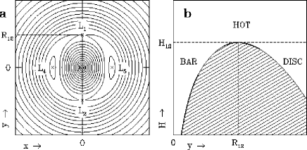
Figure 2: a) Effective potential in the $x-y$ plane of a barred disc model corresponding to Eq. (5) with $F=0.10$. The bar is along the $y$-axis and the spacing between the contours increases by a factor $1.2$ towards lower $\Phi_{\rm eff}$. The crosses indicate the Lagrangian points $L_{1/2}$ (on the $y$-axis) and $L_{4/5}$ (on the $x$-axis). b) Effective potential along the $y$-axis (thick line) and the three main classes of orbits related to the conservation of the Jacobi integral. The shaded area below the curve is forbidden for orbits with $H<H_{12}$.

In a rotating barred potential, the contours of effective potential in the plane of symmetry $z=0$ look like a volcano with a sinusoidal crest, the extrema of which defining the locations of the Lagrangian points $L_{1/2}$ and $L_{4/5}$, corresponding respectively to the saddle points and maxima of $\Phi_{\rm eff}$ on the major and minor axis of the bar (Fig. 2a). Two critical values of the Hamiltonian are associated with stars corotating at these points, namely $H_{12}\equiv\Phi_{\rm eff}(L_{1/2})$ and $H_{45}\equiv\Phi_{\rm eff}(L_{4/5})$. The first of them can be used to classify stellar orbits into three dynamical categories (Sparke & Sellwood SS (1987); Pfenniger & Friedli PF (1991)): the bar orbits and disc orbits with $H<H_{12}$, which cannot cross the $H_{12}$ contour and are therefore confined inside and outside corotation respectively, and the hot orbits with $H\geq H_{12}$, which are susceptible to cross the corotation barrier and explore all space except a small region around $L_{4/5}$ if $H<H_{45}$ (Fig. 2b). Stars with $H_{12}<H<H_{45}$ cannot cross the corotation radius at all azimuth and may therefore more likely be locked during several orbital periods on either side of corotation.

In the Solar neighbourhood, located confidently beyond corotation, only stars from the disc and hot populations are observed. Since these stars share about the same $\Phi_{\rm eff}$ if not too far from the Galactic plane, their $H$-values depend mainly on the velocities and thus one expects that the two populations occupy different regions in local velocity space. If $v$, $u$ and $w$ are measured with respect to the Galactic centre, Eq. (1) transforms into:

$$(v-R_{\circ}\Omega_{\rm P})^{2}+u^{2}+w^{2}=2(H-\Phi_{\rm eff}^{\circ}),$$ (2)

where $R_{\circ}$ is the galactocentric distance of the Sun and $\Phi_{\rm eff}^{\circ}$ the local effective potential. Thus the contours of constant Hamiltonian in velocity space are spheres centred on $(v,u,w)=(R_{\circ}\Omega_{\rm P},0,0)$ and of radius $\sqrt{2(H-\Phi_{\rm eff}^{\circ})}$ increasing with $H$. Stars on disc and hot orbits are respectively those inside and outside the $H_{12}$ sphere. If the vertical dimension is neglected, these spheres become circles with the same properties. In the axisymmetric limit and for a flat rotation curve of circular velocity $v_{\circ}$, the radius $c_{\hbox{\tiny CR}}$ of the $H_{12}=H_{45}$ contour and the low azimuthal velocity $\Delta v$ relative to $v_{\circ}$ at which this contour crosses the $u=0$ axis are then given by:

$$c_{\hbox{\tiny CR}}^{2} \equiv 2[H_{12}-\Phi_{\rm eff}(R_{\circ})]$$ (3)

$$= v_{\circ}^{2}\left[\ln{\left(\frac{R_{\hbox{\tiny CR}}}{R_{\circ}}\right)^{2}}+\left(\frac{R_{\circ}}{R_{\hbox{\tiny CR}}}\right)^{2}-1\right],$$

$$\Delta v = v_{\circ}\left(\frac{R_{\circ}}{R_{\hbox{\tiny CR}}}-1\right)-c_{\hbox{\tiny CR}},$$ (4)

where $R_{\hbox{\tiny CR}}=v_{\circ}/\Omega_{\rm P}$ is the corotation radius (see Fig. 3). For $R_{\hbox{\tiny CR}}/R_{\circ}=4.5/8$ and $v_{\circ}=200$ km s^-1, one gets $-\Delta v=0.227v_{\circ}\approx 45$ km s^-1, which coincides with the mean heliocentric asymmetric drift of the Hercules stream. Note however that this simple approximation is not truly a lower limit to the asymmetric drift of stars on hot orbits for several reasons: a non-zero $w$ velocity component defines two circles on the $H_{12}$ sphere with a reduced projected radius on the $u-v$ plane (small effect, of order $1$ km s^-1 for $|w|=20$ km s^-1), the presence of a bar lowers the effective potential at $L_{1/2}$ (larger effect, of order $5-10$ km s^-1), and finally $|\Delta v|$ is smaller if $u\neq 0$. Hence most stars in the Hercules stream are likely to fall outside the $H_{12}$ sphere and therefore may belong to the hot population.

Figure 3: Contours of constant Hamiltonian in the $u-v$ plane of a realistic 2D barred model (Eq. (5) with $R_{\hbox{\tiny CR}}/R_{\circ}=4.5/8$, $v_{\circ}=200$ km s^-1 and $F=0.20$). The velocities are relative to an inertial frame. The inner and outer solid circles give the $H_{12}$ and $H_{45}$ contours respectively, and the dotted circle is the axisymmetric limit of these contours.

From Eqs. (3) and (4), it also follows that the radius $c_{\hbox{\tiny CR}}$ and the velocity separation $|\Delta v|$ increase for larger galactocentric distances relative to $R_{\hbox{\tiny CR}}$. In particular, whatever the strength of the bar, one can always increase the fraction of the Hercules stream falling in the hot orbit region by reducing the value of $R_{\circ}/R_{\hbox{\tiny CR}}$.

4 Working potential

The analytical 2D barred potential adopted for the orbital structure analysis and the test particle simulations is the same as in D2000:

$$\Phi(R,\phi)=\Phi_{\circ}(R)+\Phi_{\rm b}(R,\phi),$$ (5)

with

$$\hskip 28.45274pt\Phi_{\circ}(R) = v_{\circ}^{2}\ln{R},$$ (6)

$$\Phi_{\rm b}(R,\phi) = \frac{1}{2}Fv_{\circ}^{2}\cos{(2\phi)}\left\{\begin{array}[]{cl}2-\left(\frac{R}{a}\right)^{3}&R\leq a\vspace*{.1cm}\\ \left(\frac{R}{a}\right)^{-3}&R\geq a.\end{array}\right.$$ (9)

This represents the sum of an axisymmetric potential $\Phi_{\circ}$ with constant circular velocity $v_{\circ}$ and a barred potential $\Phi_{\rm b}$ falling off as a quadrupole at $R\geq a$. The inner and outer parts of the latter component are described by two distinct functions which connect together at $R=a$ such as to ensure continuous potential and forces. The bar major axis is taken to coincide with the $y$-axis, contrary to the convention in D2000. The parameter $F$ is the bar strength, defined as the maximum azimuthal force on the circle of radius $a$ divided by the radial force of the axisymmetric part of the potential at the same radius (in absolute value). It is related to Dehnen’s parameter $\alpha$ by $F=8.89\alpha$. The potential is rotating at a constant pattern speed $\Omega_{\rm P}$ such as to place corotation at $R_{\hbox{\tiny CR}}=1.25a$, in agreement with numerical simulations and analyses of observations in early-type barred galaxies if $a$ is associated with the bar semi-major axis (e.g. Elmegreen BE (1996)). Unlike D2000, only flat rotation curve models will be examined. In this case, the OLR and corotation radii are related via $R_{\hbox{\tiny OLR}}=(1+1/\sqrt{2})R_{\hbox{\tiny CR}}$, and a value of $R_{\circ}/R_{\hbox{\tiny OLR}}=1.1$ corresponds to a corotation radius $R_{\hbox{\tiny CR}}=4.26$ kpc if $R_{\circ}=8$ kpc. Some considerations in the case of a non-constant rotation curve can be found in Sect. 11.

The next sections present a study of the periodic orbits outside corotation in the adopted rotating barred potential, identify the regular and chaotic regions in phase space associated with this potential, and discuss how stars may populate the available orbits. All orbits in these sections are integrated in double precision using an 8 order Runge-Kutta-Fehlberg algorithm (Fehlberg RKF (1968)). Two values of the bar strength will be considered, $F=0.10$ and $F=0.20$. The larger value corresponds to a rather strong bar (see Sect. 10 for a quantification with respect to real galaxies), but has the advantage to clearly point out the effect of chaos in the test particle simulations. Some of the key results for the intermediate case $F=0.15$ are presented in Fux (2001a ). For comparison, Dehnen’s simulations were done in the range $F=0.062-0.116$.

5 Periodic orbits

Much of the orbital structure in a system can be assessed from the study of its periodic orbits, which sometimes are considered as the skeleton of the system. While periodic orbits have been widely investigated in 2D and 3D within bars, only few papers (Athanassoula et al. ABMP (1983); Contopoulos & Grosbol CG (1989); Sellwood & Wilkinson SW (1993)) discuss them in discs surrounding bars.

Figure 4: Distinct looped periodic orbits in the axisymmetric potential $\Phi_{\circ}$ of Eq. (6) which close after one rotation in the rotating frame and are symmetric with respect to the $x$- and/or $y$-axes. The orbits all have $(H-H_{\hbox{\tiny OLR}})/v_{\circ}^{2}=0.244$ and are not drawn at the same relative scale. For cross-identification, the line thickness of the orbits is the same as for the portion of the characteristic curves in Fig. 5a to which they belong. Orbits in the lower and upper halfs of the diagram give rise to respectively stable and unstable orbits at low eccentricities when the bar is added.

A good approach to investigate periodic orbits in a 2D rotating barred potential is to start with the axisymmetric limit. In this case, the only orbits which close whatever the value of $\Omega_{\rm P}$ are the circular orbits. All other bound orbits can be thought as a libration motion around these orbits and look like a rosette which never closes, except for some exceptional potentials like a point mass with $\Omega_{\rm P}=0$, or at resonances, where the radial and azimuthal frequencies $\omega_{R}$ and $\omega_{\phi}$ satisfy the relation:

$$n_{\phi}\omega_{R}=n_{R}(\omega_{\phi}-\Omega_{\rm P}),$$ (10)

with integer values of $n_{R}\geq 0$ and $n_{\phi}$. In the rotating frame, an $n_{R}/n_{\phi}$ resonant orbit closes after $n_{R}$ radial oscillations and $|n_{\phi}|$ orbital periods. Outside corotation, $n_{\phi}$ is negative and one may speak of outer $n_{R}/|n_{\phi}|$ resonances. This paper discusses only outer resonances and the minus sign in their labelling will be omitted. While in the axisymmetric case the orientation of the resonant orbits is arbitrary, the virtual introduction of a bar will retain only those orbits which are reflection symmetric with respect to (at least one of) the bar principal axes, say the $x$- and $y$-axes. Figure 4 displays several orbits of this kind with $|n_{\phi}|=1$. There exists an infinity of resonant orbits which accumulate at corotation as $n_{R}\rightarrow\infty$. Those with $n_{R}>6$ or closing after more than one rotation will not be considered in this paper. For even $n_{R}$, there exists two distinct resonant orbits for each value of the Hamiltonian, depending on whether the $x$-axis coincides with orbital apocentre or pericentre. For odd $n_{R}$, there are twice as many solutions because the orbits are no longer reflection symmetric with respect to both axes.

Figure 5: a) Characteristic diagram in the rotating axisymmetric potential (Eq. (6)) for the circular orbit (circ.) and the lowest order outer $n_{R}/1$ resonant orbits which are symmetric with respect to the coordinate axes. The curves give the $x$-coordinate normalised by the OLR radius of the orbits when they cross the $x$-axis with $\dot{y}>0$ as a function of the Hamiltonian value relative to $H_{\hbox{\tiny OLR}}$, the $H$-value of the circular orbit at the OLR, and normalised by $v_{\circ}^{2}$, assuming that the potential rotates clockwise in the inertial frame. The short-dashed line gives the zero velocity curve (ZVC) and the vertical dotted line the $H$-value of the orbits sketched in Fig. 4. The grey $3/1$ and $5/1$ resonance curves are shown only in the lower frame, which is a magnification of the rectangular box in the upper frame. b) Corresponding characteristic diagram in the barred potential of Eq. (5) with a bar strength $F=0.10$. The major axis of the bar coincides with the $y$-axis. The full and dotted parts of the curves stand for stable and unstable orbits respectively. The orbit labels refer to the nomenclature of Contopoulos & Grosbol (CG (1989)). The symmetric and asymmetric $3/1$ and $5/1$ resonance curves are plotted with grey lines in both the upper and lower frames, but labelled only in the lower one. c) Same as former diagram, but with $F=0.20$.

The characteristic curves of these resonant orbits in the $H-x$ plane (Fig. 5a) all intersect the circular orbit curve (COC) at their point of lowest $H$, corresponding to a bifurcation. For even resonances, four branches emanate from the bifurcation, two from the COC and two from the resonance curve. The resonance branches above (towards larger $x$) and below the COC represent orbits with respectively apocentre and pericentre on the $x$-axis. The lower branch always passes through the zero velocity curve (ZVC), where the orbit becomes cuspy on the $x$-axis and then develops loops at higher value of the Hamiltonian. For such loop orbits, the $x$-coordinate of the characteristic curves does not trace the pericentre but the place where the orbit self-intersect and $\dot{x}\neq 0$. For odd resonances, the bifurcation has six branches: the two from the COC, two for the resonant orbits with radial extrema on the $x$-axis and which have properties similar to the former even resonance branches, and two for the resonant orbits with those extrema on the $y$-axis. The two latter branches have opposite $\dot{x}$ but degenerate into the same curve in the $H-x$ characteristic diagram. All periodic orbits in the symmetry plane of an axisymmetric potential are stable.

Figures 5b and 5c show how the characteristic curves are modified when the bar component with major axis on the $y$-axis is added to the potential. The changes mainly occur at the bifurcations of the axisymmetric case. The bifurcations of the even resonances become gaps, with the right (low $H$) COC branch deviating into the lower resonance branch, and the upper resonance branch into the left COC branch, giving rise to a sequence of continuous orbit families. In the terminology introduced by Contopoulos & Grosbol (CG (1989)), the outermost of these families is called $x_{1}(1)$, and the other families are divided into an upper $x_{1}^{*}(i)$ and a lower $x_{1}(i)$ sub-family at or near the point of minimum $H$, where the stability of the orbits appears to reverse. The six-branch bifurcations of the odd resonances (see the $1/1$ and $3/1$ resonances in the figures) split into two pitchfork bifurcations, one involving the resonant orbits symmetric with respect to the bar minor axis, which are stable near the bifurcation, and the other the resonant orbits non-symmetric relative to this axis, which are unstable near the bifurcation and qualified as asymmetric. As a by-product of this splitting, the segment of the $x_{1}(i)$ characteristic curve between the two new bifurcations becomes unstable.

Figure 6: Orbits of the $x_{1}(1)$ (left) and $x_{1}(2)$ (right) families in the model with bar strength $F=0.10$, with the thick line representing the orbit of lowest apocentre and of lowest Hamiltonian respectively. The shaded ellipse sketches the bar. The full and dotted lines represent stable and unstable orbits respectively. The nearly circular $x_{1}(1)$ orbits extend out to infinity. Note the unstable $x_{1}(1)$ orbit at the $1/1$ resonance.

At low eccentricity (i.e. small $H$), only those orbits with a pericentre on the bar minor axis seem to be stable. This could be the influence of the Lagrangian points $L_{\rm 4/5}$, which are stable fix points in the models. At high eccentricity, all orbit families undergo a change of stability and the characteristic curves in Fig. 5 are all interrupted at the point where the minor axis loop of the orbits touches the centre $R=0$. The curves actually go beyond this point, but the resonance number changes. For instance, the $2/1$ orbits become $2/3$ orbits. When increasing the bar strength (from Fig. 5b to Fig. 5c), the resonance gaps between successive $x_{1}(i)$ curves and the separation between the pitchfork bifurcation pairs increases. The characteristic curves also become more twisted and the fraction of stable orbits decreases. In particular, almost all $x_{1}(3)$ orbits are unstable for $F=0.20$. It should be noted that other authors (Athanassoula et al. ABMP (1983); Sellwood & Wilkinson SW (1993)) report more complicated characteristic curves for the $x_{1}(2)$ and higher order orbit families near the ZVC in their models, probably as a consequence of an $m=4$ Fourier component in the potential.

Some orbits of the above families are plotted in D2000, but obviously missing all eccentric $x_{1}(1)$ and $x_{1}(2)$ orbits with loops on the bar minor axis. A more complete set of orbits from these two families are given in Fig. 6. These orbits are the most important even $n_{R}$ periodic orbits because they are usually associated with the largest invariant curve islands in surface of section maps. The orbits drawn with thick lines are examples of the perpendicularly oriented orbits that replace the circular orbit near the OLR radius and which have been proposed as a possible explanation for either the Hyades and Sirius streams (Kalnajs K (1991)) or the Hercules-LSR bimodality (D2000) in the observed $u-v$ distribution. As we shall see in the next sections, the stable eccentric $x_{1}(1)$ orbits also play an important role in shaping the local velocity distribution. Regular orbits trapped around them are indeed unlikely to be heavily populated by stars, but represent forbidden phase space regions for chaotic orbits.

The space coverage of the orbit families can be determined from $x-y$ plots like in Fig. 6. For each position in real space, there will be an (infinite) set of periodic orbits passing through. The velocity trace in planar velocity space of the above described orbits, as well as the curves delineating some of the main resonances in the underlying axisymmetric potential, are indicated in Figs. 7 and 8 for various azimuthal angles $\varphi$ and a realistic range of galactocentric distances relative to the OLR, and for two different bar strengths. Here the angle $\varphi$ is measured from the bar major axis and increases towards the direction opposite to galactic rotation, i.e. coincides with the traditional in-plane inclination angle of the bar. All space positions are reached by many of the considered orbit families, and sometimes several traces are produced by orbits from the same family: for instance, at $\varphi=90^{\circ}$, there is a large range of $R$ with three traces from $x_{1}(1)$ orbits, mainly due to the loops on the $x$-axis of the high-$H$ orbits. The traces of the $1/1$, $1/1$ asym, $x_{1}(1)$, $x_{1}^{*}(2)$, $x_{1}(2)$ and $x_{1}^{*}(3)$ orbits with non-nearly vanishing $|u|$-velocity all fall very close to the associated resonance curves, indicating that the axisymmetric approximation used to compute these curves works well for $n_{R}\leq 4$. Not all resonant periodic orbits, i.e. those with traces on the resonance curves, are unstable. In particular, orbits on the $2/1$ (OLR) and $1/1$ resonance curves are stable $x_{1}(1)$ and $1/1$ orbits at $\varphi=90^{\circ}$ and unstable $x_{1}^{*}(2)$ and $1/1$ asym orbits at $\varphi=0^{\circ}$, except for a $x_{1}^{*}(2)$ and a $x_{1}(1)$ orbit with $u=0$ for $R/R_{\hbox{\tiny OLR}}\geq 1.1$. Hence resonance regions of phase space are not necessary unstable and depleted as asserted in D2000 for the OLR.

There are sometimes several orbits from the same family plotted very close to each other, like for example the three unstable $x_{1}(2)$ orbits at $R/R_{\hbox{\tiny OLR}}=0.9$, $\varphi=30^{\circ}$ and $(v/v_{\circ},u/v_{\circ})\approx(-0.85,-0.80)$ for $F=0.20$. This happens when the sequence of orbits within the family reverses its progression in the $x-y$ plane towards a given direction and very close to the current space position, causing an accumulation of orbits near this position with different local velocities. One may also note that the continuous transitions between some orbit families can cause periodic orbits from different families to have almost identical traces, as for example the $x_{1}^{*}(2)$ and $x_{1}(2)$ near the centre of the frame $R/R_{\hbox{\tiny OLR}}=1.1$ and $\varphi=90^{\circ}$ in Fig. 8.

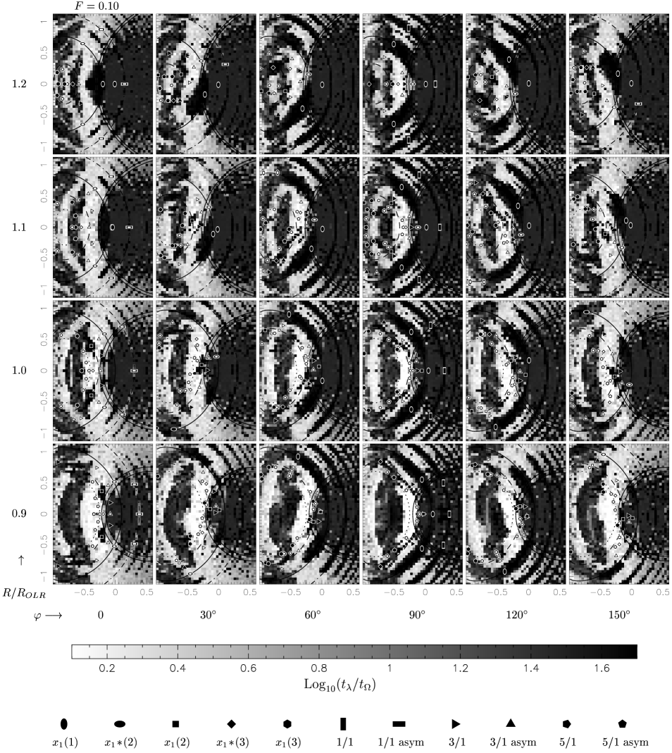
Figure 7: Liapunov divergence timescale of the orbits in the $u-v$ plane as a function of position in real space, for a bar strength $F=0.10$. The horizontal and vertical axes of each frame are $v/v_{\circ}$ and $u/v_{\circ}$ respectively, with $v$ positive in the direction of rotation and $u$ towards the anti-centre, and the origin at the circular orbit of the axisymmetric part of the potential $\Phi_{\circ}$. The timescales are in units of local circular period $t_{\Omega}$ in $\Phi_{\circ}$ and greyscale coded. The dark and white regions respectively represent regular and chaotic orbits. The oval and polygonal symbols indicate the positions of the periodic orbits, with a different symbol for each orbit family. Full and empty symbols respectively stand for stable and unstable orbits. The full lines open towards the right (increasing $v$) are the $H_{12}$ and $H_{45}$ contours. The dash-dotted, solid, dashed and dotted lines open towards the left respectively give the locations of the outer $1/1$, $2/1$, $4/1$ and $6/1$ resonant orbits in $\Phi_{\circ}$.

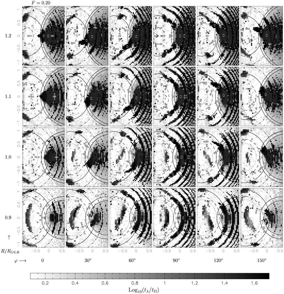
Figure 8: As Fig. 7, but for a bar strength $F=0.20$.

The rather large number of stable simple periodic orbits through each space position and the numerous stellar streams observed in the Solar neighbourhood may suggest that at least some of them are related to periodic orbits, as anticipated in Kalnajs (K (1991)). For instance, beside the idea of the $x_{1}(1)$ and low-eccentricity $x_{1}(2)$ induced streams near the OLR radius, the $\varphi=30^{\circ}$ frames in Fig. 7 betray interesting stable eccentric $x_{1}(2)$ and $5/1$ asym orbits at $R/R_{\hbox{\tiny OLR}}=1.2$ and $R/R_{\hbox{\tiny OLR}}=1.1$ respectively and with $v/v_{\circ}\approx-0.6$ and $u/v_{\circ}\approx 0.05-0.15$, which fall very close to the velocity of the young Arcturus stream (see Table LABEL:stream).

6 Liapunov exponents

The next step after the periodic orbit search is to determine the phase space extent of the regular orbits trapped around the stable closed orbits and of the chaotic orbits, which have no other integral than the Jacobi integral. The Poincaré surface of section method is well suited to highlight the regular and chaotic regions in phase space at constant value of the Hamiltonian, but not at constant position in real space. A better tool for this purpose are the Liapunov exponents, which also allow to quantify the degree of stochasticity of the orbits. These exponents describe the mean exponential rate of divergence of two trajectories initially close to each other in phase space and are defined as:

$$\lambda(\@vec{x}_{\circ},\Delta\@vec{x}_{\circ})=\lim_{\scriptsize\begin{array}[]{c}\Delta\@vec{x}_{\circ}\rightarrow 0\\ t\rightarrow\infty\end{array}}\frac{1}{t}\ln{\frac{|\Delta\@vec{x}(t)|}{|\Delta\@vec{x}_{\circ}|}},$$ (11)

where $\@vec{x}_{\circ}$ and $\Delta\@vec{x}_{\circ}$ are the initial ($t=0$) position and deviation, and $\Delta\@vec{x}(t)$ is the deviation at time $t$. Such limit is proven to exist and is finite for all bound orbits (Oseledec O (1968)). The value of $\lambda$ generally depends on the direction of the deviation $\Delta\@vec{x}_{\circ}$ and, if $N$ is the dimension of phase space, one can show (Oseledec O (1968); Benettin et al. BGS0 (1976)) that there exists in fact $N$ discrete exponents $\lambda_{1}\geq\lambda_{2}\geq\ldots\geq\lambda_{N}$. However, the largest exponent $\lambda_{1}$ is the most important because it results from almost all deviations in $\Delta\@vec{x}_{\circ}$-space (e.g. Udry & Pfenniger UP (1988)), and therefore is the one found in practice when the initial deviation is chosen randomly. Moreover, this exponent exclusively determines the orbital stability: if $\lambda_{1}=0$, all exponents vanish and the orbit is regular, and if $\lambda_{1}>0$, the orbit is chaotic and the amount of chaos increases with $\lambda_{1}$.

The numerical computation of the Liapunov exponents faces some problems related to the limits in Eq. (11). First, the finite initial deviation $\Delta\@vec{x}_{\circ}$ may rapidly grow as large as the size of the orbits themselves, especially for chaotic orbits, and thus $\Delta\@vec{x}(t)$ must be occasionally scaled down by a large factor. Noting $\Delta\@vec{x}^{0}(t)$ the deviation before the first rescaling, this is done in a way similar to Contopoulos & Barbanis (CB (1989)), by normalising $\Delta\@vec{x}(t)$ to $|\Delta\@vec{x}_{\circ}|$:

$$\Delta\@vec{x}^{i}(t_{i})=\frac{|\Delta\@vec{x}_{\circ}|}{|\Delta\@vec{x}^{i-1}(t_{i})|}\Delta\@vec{x}^{i-1}(t_{i})$$ (12)

every time $t_{i}$ when $|\Delta\@vec{x}^{i-1}|>1.3\cdot 10^{-3}R_{\hbox{\tiny OLR}}$, so that after $n$ iterations:

$$\ln{\frac{|\Delta\@vec{x}(t)|}{|\Delta\@vec{x}_{\circ}|}}=\ln{\frac{|\Delta\@vec{x}^{n}(t)|}{|\Delta\@vec{x}_{\circ}|}}+\sum_{i=1}^{n}\ln{\frac{|\Delta\@vec{x}^{i-1}(t_{i})|}{|\Delta\@vec{x}_{\circ}|}}.$$ (13)

Another problem is that one cannot integrate orbits over an infinite time and thus the time limit in Eq. (11) must be replaced by the value at some finite time, which has been set to about $3$ Hubble times when the models are scaled to realistic physical units.

The Liapunov exponent $\lambda_{1}$ has been calculated on a Cartesian grid of planar velocities for different positions of the observer, using the 2D potential of Eq. (5) and with an initial deviation of $+1.3\cdot 10^{-11}R_{\hbox{\tiny OLR}}$ in the $R$-coordinate (Figs. 7, 8 and 10). The results are presented as a divergence timescale $t_{\lambda}\equiv 1/\lambda_{1}$ in units of local circular period in the axisymmetric part of the potential, which provides a more obvious and useful measure of stochasticity. Diagrams have been computed for every $10^{\circ}$ in azimuth for $R/R_{\hbox{\tiny OLR}}=$ 0.9, 1.0, 1.05, 1.1, 1.2 and also at $\varphi=25^{\circ}$ over a larger radial range, but those diagrams between our $30^{\circ}$ sampling and at $R/R_{\hbox{\tiny OLR}}=1.05$ will not be shown here (and the same is true for the velocity distributions of the next section). We shall refer to such diagrams as “Liapunov” diagrams.

The first thing to notice in these diagrams is that the stable and unstable periodic orbits fall within regular and chaotic regions respectively, as expected. There are some apparent exceptions like the $1/1$ asym orbit at $\varphi=0$ and large $R$ which must owe to the limited velocity resolution of the diagrams ($=0.04v_{\circ}$; see Fux 2001b for some higher resolution Liapunov diagrams). The fraction of chaotic orbits also obviously increases with bar strength. Furthermore, as a consequence of the four-fold symmetric barred potential, the diagrams at $\varphi=0$ and $90^{\circ}$ are symmetric with respect to $u=0$ and, more generally, diagrams at supplementary angles are anti-symmetric to each other in $u$, i.e. $t_{\lambda}(R,180^{\circ}-\varphi,v,u)=t_{\lambda}(R,\varphi,v,-u)$.

At $\varphi=90^{\circ}$ and for the radial range explored in Figs. 7 and 8, the $2/1$ and $1/1$ resonance curves, as well as all other not highlighted resonances of the form $2/|n_{\phi}|$ with integer $|n_{\phi}|$, are embedded in the middle of broad regular orbit arcs separated by mainly chaotic regions which come closer to $u=0$ as the bar strength increases. For $R/R_{\hbox{\tiny OLR}}\ga 1.1$ (and $\varphi=90^{\circ}$), the regularity of the OLR arc gets destroyed near $u=0$, leaving the place to an unstable $x_{1}^{*}(2)$ orbit. Between the dominant regular orbit arcs, secondary regular arcs associated with resonances of the form $4/|n_{\phi}|$ with odd integer $|n_{\phi}|$ can also be identified, especially for $F=0.10$. This includes in particular the $4/1$ resonance arc visible for $R/R_{\hbox{\tiny OLR}}\la 1.0$. In fact, the chaotic regions between the broad resonance arcs are probably densely filled by tiny arcs of higher order regular resonant orbits, but the filling factor must be very low.

At $\varphi=0$, the situation is reversed: the $2/|n_{\phi}|$ resonance curves lie in chaotic regions at large $H$ which are spaced by regular orbit arcs right between the resonances. At intermediate angles, the regular and chaotic regions become offset from the resonance curves and the $u$-symmetry breaks. In particular, for $\varphi\sim 30^{\circ}$ and $R/R_{\hbox{\tiny OLR}}\ga 1.0$, i.e. realistic positions for the Sun, an extreme case of asymmetry arises near the OLR: a prominent region of regular orbits extends down to negative $u$, bounded roughly by the OLR curve on the right and penetrating well inside the hot orbit zone, whereas the positive $u$ part of the OLR curve is surrounded by a wide chaotic region extending somewhat inside the $H_{12}$ contour and coinciding very well with the $u-v$ location of the Hercules stream.

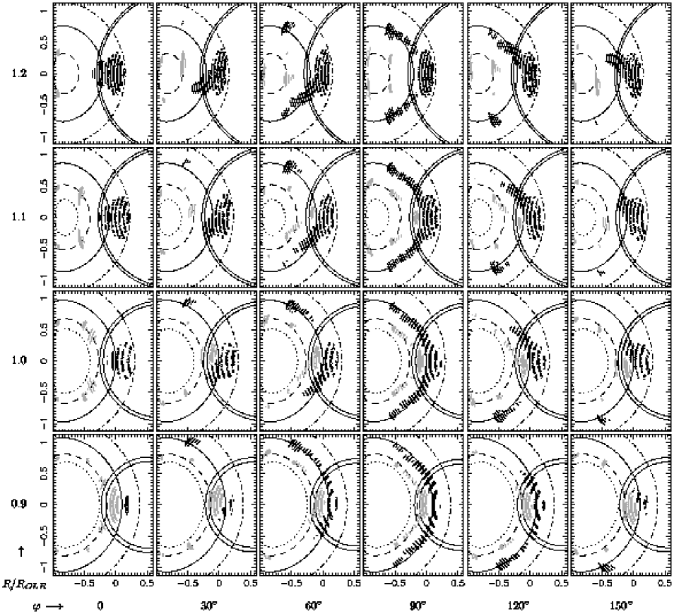
Figure 9: Location in the $u-v$ plane of the regular orbits trapped around the stable $x_{1}(1)$ periodic orbits for a bar strength $F=0.20$ (dark points) and around the stable $x_{1}(2)$ orbits for $F=0.10$ (grey points). The computational details are described in the text. The horizontal and vertical axes of the frames and the different curves are as in Fig. 7. The $H$-contours are given for $F=0.10$.

Figure 9 shows the $u-v$ region occupied by the regular orbits trapped around the stable $x_{1}(1)$ and $x_{1}(2)$ periodic orbits. To construct this figure, we have first derived many surfaces of section at mainly constant Hamiltonian interval $\Delta H=0.054v_{\circ}^{2}$ to locate the islands of invariant curves around these periodic orbits. Then the orbits within each islands of these maps have been sampled by 50 regularly spaced points along a straight line across the central periodic orbit and within the outermost invariant curve of the island. Finally, all the resulting initial conditions are integrated for 20 rotations in the rotating frame and the velocities are plotted when the orbits pass within a distance of $d_{\rm max}=R_{\circ}/80$ of the considered space positions. The striped appearance of the regular $x_{1}(1)$ and $x_{1}(2)$ regions in the diagrams are due to the discrete $H$-sampling and the broadening of the stripes to the finite value of $d_{\circ}$ (not to an inaccurate orbital integration). The islands in the surfaces of section generally contain sub-resonances which have been included. The $x_{1}(1)$ islands however have been truncated at the $1/1$ resonance, so that the part of the $x_{1}(1)$ region on the high-$v$ side of the $1/1$ resonance curve is not represented in the $u-v$ diagrams. The $x_{1}(1)$ regions are derived for $F=0.20$ because the high level of chaos at this bar strength makes it easier to distinguish the boundaries of these regions in the surfaces of section, and the $x_{1}(2)$ regions for $F=0.10$ in order to emphasise the more regular case where these regions are larger.

From this figure, it is obvious that the regular orbit arcs near the OLR, and in particular the prominent regular region at $\varphi\sim 30^{\circ}$ and $R/R_{\hbox{\tiny OLR}}\ga 1.0$ discussed previously, are produced by the regular orbits around the stable periodic orbits of the $x_{1}(1)$ family, with an eccentricity increasing towards larger Hamiltonian values. The regular regions associated with the stable $x_{1}(2)$ orbits can be viewed as divided into two parts, one involving only low-eccentricity orbits and the other one the higher eccentricity orbits falling close to the $4/1$ resonance curve. The low-eccentricity orbit part exists for $R/R_{\hbox{\tiny OLR}}\la 1.1$ and over an angle range around $\varphi=90^{\circ}$ increasing as $R$ decreases, and is generally enclosed between the $H_{12}$ contour and the OLR curve. Elsewhere, it is dissolved and only an unstable $x_{1}^{*}(2)$ orbit remains (Fig. 7). The higher eccentricity part connects the low-eccentricity part at $R/R_{\hbox{\tiny OLR}}\approx 0.9$ and then progressively detach from it as the $4/1$ resonance curve moves away from the $H_{12}$ contour at larger $R$. In particular, for $R/R_{\hbox{\tiny OLR}}\ga 1.1$ and for $F=0.10$, there are no regular quasi-$x_{1}(2)$ orbits between the $H_{12}$ contour and azimuthal velocities less than $v/v_{\circ}=-0.35$, whatever the angle $\varphi$, and no low-eccentricity such orbits at all for $\varphi\la 50^{\circ}$. Hence for this bar strength, the Hercules-like mode found in D2000’s simulations at $R/R_{\hbox{\tiny OLR}}\approx 1.1$ and $\varphi\sim 25$ cannot be related to such quasi-$x_{1}(2)$ orbits.

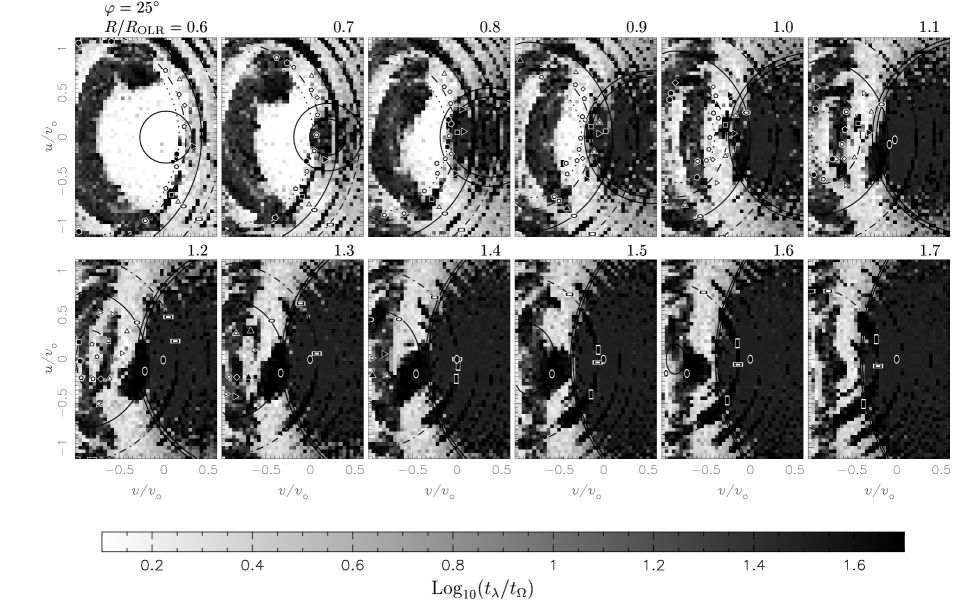
Figure 10: As Fig. 7, but for $\varphi=25^{\circ}$ and $0.6\leq R/R_{\hbox{\tiny OLR}}\leq 1.7$.

Figure 10 provides Liapunov diagrams over a larger radial range at $\varphi=25^{\circ}$ and for $F=0.10$. These diagrams clearly show that the $H_{12}$ contour marks the average transition between regular and chaotic motion. Hence disc orbits are essentially regular and hot orbits essentially chaotic. The diagrams in Fig. 10 also nicely illustrate the dependence of the $H_{12}$ and $H_{45}$ contours with galactocentric distance discussed in Sect. 3, and show how the velocity spacing between these contours decreases with increasing $R$.

Martinet & Raboud (MR (1999)) have computed a diagram $\Delta(v,u)$ representing the relative pericentre deviation between planar orbits integrated in a barred $N$-body model and the corresponding orbits in the underlying axisymmetric potential, starting from a realistic space position of the Sun. Their diagram correlates well with our Liapunov diagrams in the sense that the larger values of $\Delta$ coincide with shorter Liapunov timescales. In particular, a clear jump of $\Delta$ occurs at $H\approx H_{\rm 12}$, with the high-$H$ side displaying much larger pericentre deviations on the average, and there is also a tail of small $\Delta$-values at negative $u$ extending inside the hot orbit region.

It is worth mentioning that in a two-dimensional axisymmetric potential, all orbits are regular, i.e. have vanishing $\lambda_{1}$. Hence the chaotic regions discussed here are all produced by the influence of the bar alone. Also, the divergence timescale $t_{\lambda}$ in the chaotic regions may be as low as a few orbital times. This property may have important consequences on the early evolution of the distribution function in barred galaxies, as we shall see in the following section.

7 Phase space crowding

Given the orbital structure of phase space, we now want to know how nature populates the available orbits. This is done resorting to test particle simulations with the following two integral initial distribution function (Dehnen 1999a ):

$$f_{\circ}(E,L_{z})\!=\!\frac{2\Omega(R_{\rm c})}{\kappa(R_{\rm c})}\frac{\tilde{\Sigma}(R_{\rm c})}{2\pi\tilde{\sigma}(R_{\rm c})}\exp{\!\left[\Omega(R_{\rm c})\frac{L_{z}\!-\!L_{\rm c}(E)}{\tilde{\sigma}^{2}(R_{\rm c})}\right]},$$ (14)

where $E$ and $L_{z}$ are respectively the energy and the $z$-component of the angular momentum, $R_{\rm c}(E)$ and $L_{\rm c}(E)$ the radius and angular momentum of the circular orbit with energy $E$, $\Omega$ and $\kappa$ the circular and epicycle frequencies, and $\tilde{\Sigma}(R)$ and $\tilde{\sigma}(R)$ the approximate surface density and radial velocity dispersion profiles. This is a modified Shu (S (1969)) distribution where the radius of the guiding centre $R_{\rm c}$ is deduced from the energy instead of the angular momentum, with the main advantage that the density function extends smoothly towards negative $L_{z}$. Adopting $\tilde{\Sigma}(R)\sim\exp{(-R/h_{R})}$ and $\tilde{\sigma}^{2}(R)=\tilde{\sigma}_{\circ}^{2}\exp{(-(R-R_{\circ})/h_{\sigma})}$, where $R_{\circ}$ is the galactocentric distance of the Sun and $\tilde{\sigma}_{\circ}$ the approximate velocity dispersion at that distance, the initial distribution function has three free parameters, which unless otherwise specified are set to $h_{R}/R_{\circ}=0.33$, $\tilde{\sigma}_{\circ}/v_{\circ}=0.2$ and $h_{\sigma}/R_{\circ}=1.0$. This results in exactly the same initial conditions as for the default flat rotation curve case in D2000. In the beginning of the simulations, the non-axisymmetric part of the potential is gradually switched on from no contribution at $t=0$ to its full value at $t=2t_{\rm b}$, where $t_{\rm b}=2\pi/\Omega_{\rm P}$ is the rotation period of the bar, exactly the same way as in D2000 for the simulations with default integration time.

For the time integration, D2000 uses a subtle backward integration technique based on the conservation of the phase space density along the orbits in collisionless systems. The idea is to integrate back in time until $t=0$ the phase space points on a Cartesian grid of $u-v$ velocities at a given space position $(R_{\circ},\varphi)$ and time $t_{\rm end}$, to determine the energy $E$ and angular momentum $L_{z}$ of the originating orbits in the initial axisymmetric potential, and from these infer $f(t_{\rm end},R_{\circ},\varphi,v,u)=f_{\circ}(E,L_{z})$. The advantages of this technique is that only the orbits strictly necessary to derive the evolved local velocity distributions need to be computed, and that these velocity distributions are not affected by Poisson noise. Moreover, a unique simulation suffices to get $u-v$ distributions for different initial conditions, because $f_{\circ}$ comes in only after the orbit integration.

Unfortunately, the backward integration technique faces two major problems illustrated in Fig. 11, which shows the long term evolution of the planar velocity distribution at $R_{\circ}/R_{\hbox{\tiny OLR}}=1.1$ and $\varphi=25^{\circ}$ using this technique. The integration time in D2000 ranges from $4$ bar rotation for most simulations, corresponding to only $\sim 2$ orbital periods at $R=R_{\circ}$ in the inertial frame, up to $8$ bar rotation for some cases, but always matching the growth time of the bar to half the total integration time. The frame at $t=4t_{\rm b}$ is similar to his results, revealing a clear bimodal distribution. However, at $t=10t_{\rm b}$, the valley between the two modes becomes heavily populated, destroying the bimodality, and at later times, incurved waves appear in this valley with a spacing between the maxima decreasing with time. This is a typical signature of ongoing phase mixing in a regular region of phase space, which here corresponds to the eccentric orbit part of the quasi-$x_{1}(1)$ region according to the previous section. A very similar phenomenon, with similarly incurved waves, can also be barely recognised near the $1/1$ resonance. Between the $2/1$ and $1/1$ resonances, phase mixing operates on a shorter timescale and the orientation of the wave fronts seems to change from nearly-vertical at $t=30t_{\rm b}$ to nearly-horizontal at $t=120t_{\rm b}$. The backward integration technique in fact yields the fine-grained distribution function, which never smoothes out on sufficiently small scales, whereas the physical one to compare with the observations is the coarse-grained distribution. The second problem is related to chaos: at $t\ga 30t_{\rm b}$, the $u-v$ distribution becomes noisy in the chaotic regions because the phase space points integrated backwards from these regions sample the initial distribution function more randomly. Hence much longer integration times than in D2000 are required to obtain quasi-equilibrium (coarse-grained) distribution functions and to properly take into account the effect of chaos (remember that the divergence timescales for chaotic orbits is of the order of several orbital periods), and one cannot escape the fate of smoothing the fine-grained distribution.

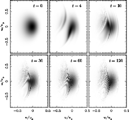
Figure 11: Time evolution of the velocity distribution in the $u-v$ plane at $R_{\circ}/R_{\hbox{\tiny OLR}}=1.1$ and $\varphi=25^{\circ}$ using the backward integration technique. The bar strength is $F=0.10$ and the time is given in units of the bar rotation period $t_{\rm b}$.

Figure 12: Velocity distribution in the $u-v$ plane as a function of space position in the test particle simulations with a bar strength $F=0.10$. The distributions are time averages within the interval from $25$ to $35$ bar rotations after the beginning of the simulations. The velocity contours are as in Fig. 1, whereas the axis labels, the Hamiltonian contours, the resonance curves and the periodic orbits are as in Fig. 7.

Therefore, most of the test particle simulations in this paper were done by simple forward integration. The initial phase space density is sampled by $N$ particles which are then integrated forward in time, and the $u-v$ diagrams at space position $(R_{\circ},\varphi)$ are constructed from all the particles within a distance $d_{\rm max}=R_{\circ}/80$ from that position (corresponding to $d_{\rm max}=100$ pc for $R_{\circ}=8$ kpc), using a Cartesian velocity binning with a bin size of $0.005v_{\circ}$. To increase the particle statistics, the $u-v$ distributions are averaged over 10 bar rotations and then smoothed within a square of $11\times 11$ bins. The time average, which is hardly possible in the backward integration technique, is also very convenient to reduce the phase mixing problem, as the contribution of each particle to a $u-v$ distribution becomes proportional to the time the particle spends within the volume where the distribution is computed. With the forward integration technique, the time evolution of the velocity distribution can be followed within a unique simulation. The test particle simulations of this paper all have $N=10^{6}$ and the velocity distributions have been derived within two time intervals, $25\leq t/t_{\rm b}\leq 35$ and $55\leq t/t_{\rm b}\leq 65$. Since the distance parameters in $f_{\circ}$ scale as $R_{\circ}$ and not $R_{\hbox{\tiny OLR}}$, the results at different $R_{\circ}/R_{\hbox{\tiny OLR}}$ require distinct simulations.

Figure 13: Same as Fig. 12, but for a bar strength $F=0.20$ and a time average over the interval $55\leq t/t_{\rm b}\leq 65$.

Figure 12 shows the $u-v$ distributions at various space positions averaged over the time interval $25\leq t/t_{\rm b}\leq 35$ for a bar strength $F=0.10$. As for the Liapunov diagrams, the distributions are obviously symmetric with respect to $u=0$ for $\varphi=0$ and $\varphi=90^{\circ}$ and the distributions at same radius but supplementary angles are anti-symmetric to each other in $u$. This is clearly not the case in the simulations of D2000 (see his figure 2, where $F=0.089$), providing a further argument that these have not achieved a quasi-stationary regime. Moreover, the traces of the stable $x_{1}(1)$ periodic orbits away from the $2/1$ resonance curve lie closer to the high angular momentum peak of the velocity distributions. For this bar strength and the adopted values of the parameters in the initial distribution function, there is also no clear bimodality with a deep separation valley at $R_{\circ}/R_{\hbox{\tiny OLR}}\ga 1.1$ and near $\varphi=30^{\circ}$, although a clear density excess remains at low $v$ and positive $u$. However, all space positions where a low-eccentricity regular $x_{1}(2)$ region exists (see former section and Fig. 9) present a nice bimodality, with the low angular momentum mode coinciding very well with that region and always peaking inside the $H_{12}$ contour.

While the traces of the non-resonant $x_{1}(1)$ and $x_{1}(2)$ orbits are generally embedded within their associated quasi-periodic orbit modes, they do not necessarily exactly coincide with the peak of these modes, especially in the $x_{1}(2)$ case (e.g. $R_{\circ}/R_{\hbox{\tiny OLR}}=1.0$ and $\varphi=60^{\circ}-120^{\circ}$ in Fig. 12). Furthermore, since the quasi-periodic orbits cover a larger space area than the periodic orbits themselves, quasi-$x_{1}(1)$ and quasi-$x_{1}(2)$ modes may occur even at positions where no $x_{1}(1)$ or $x_{1}(2)$ orbit are passing through.

Increasing the bar strength (Fig. 13) provides a better understanding of how the velocity distributions are affected by chaos. Now, there appears to be an obvious second source producing a low angular momentum mode, which adds to the quasi-$x_{1}(2)$ orbit flow at the space regions reached by these orbits, and acts alone elsewhere, as for instance at $R_{\circ}/R_{\hbox{\tiny OLR}}=1.1$ and $\varphi=30^{\circ}$. The overdensity in velocity space generated by this second source correlates very well with highly stochastic regions in the Liapunov diagrams (see Fig. 8) and seems to always peak outside the $H_{12}$ contour. At $\varphi=90^{\circ}$, the overdensity culminates at $u\approx 0$ and is enclosed by the regular arc of eccentric quasi-$x_{1}(1)$ orbits. At $\varphi=0$, these quasi-$x_{1}(1)$ orbits occupy the $u=0$ region and chaotic overdensities happen symmetrically on both positive and negative $u$ sides of this region. At $\varphi\sim 30^{\circ}$, the quasi-$x_{1}(1)$ region is located at negative $u$ and there is a large chaotic overdensity at positive $u$.

These properties result from the decoupling between the regular and the chaotic regions of phase space. Since chaotic orbits cannot visit the regions of regular motion and, vice versa, regular orbits avoid the chaotic regions, the distribution function in each of these regions evolves in a completely independent way. In the regular regions, it recovers roughly the initial distribution after phase mixing, whereas in the chaotic regions, it is substantially modified through a process known as chaotic mixing and which operates on the Liapunov divergence timescale (e.g. Kandrup HEK (2001)): the particles on chaotic orbits quickly disperse within the easily accessible phase space regions, i.e. not impeded by cantori or an Arnold web, and converge towards a uniform population of these regions. The dominant manifestation of chaotic mixing is a net migration of particles from the inner to the outer space regions. For instance, in the simulations with $R_{\circ}/R_{\hbox{\tiny OLR}}=1.1$, the scale length of the radial particle distribution, which remains very close to an exponential in the range $0.5\la R/R_{\circ}\la 1.25$, increases by $\sim 30$% for $F=0.10$ and by $\sim 90$% for $F=0.20$ within this radial range. This migration is particularly marked for particles on hot chaotic orbits because the region inside corotation initially represents a large reservoir of such particles and because these particles can freely pass over corotation. As a consequence, in the explored $R_{\circ}/R_{\hbox{\tiny OLR}}$ range, the chaotic regions in the $u-v$ diagrams are more heavily crowded than the regular regions at $H\ga H_{12}$, therefore corresponding to local overdensities.

At first glance, there seems to be a rather continuous transition from the quasi-$x_{1}(2)$ orbit mode to the main chaotic orbit mode when moving across the OLR radius towards increasing $R_{\circ}$, with always a single effective peak showing up and with the involved quasi-$x_{1}(2)$ region progressively dissolving in the chaotic one. But in some cases, the two mode-generating sources really contribute to distinct peaks in the velocity distribution (see Fig. 20d for an example).

The process of chaotic mixing leads to velocity distribution contours which are parallel to the contours of constant $H$ in the chaotic regions (e.g. Fig. 13). This property is also consistent with Jean’s theorem stating that the distribution function in a steady-state system depends only on the integral of motions. The only integral for the chaotic orbits in the present 2D barred models is the value of the Hamiltonian, hence the distribution function and therefore the corresponding velocity distributions at fixed space position should be a function of only $H$ in the chaotic regions. It should be noted that the Jeans theorem does not strictly apply to the hot and disc chaotic orbits. Indeed, these orbits are not energetically bound (in terms of $H$) and thus the phase space density around such orbits and within the finite space volume of the galaxy should decrease with time, conflicting with the steady-state assumption of the theorem. However, the escaping timescale of these chaotic orbits, which is essentially controlled by Arnold diffusion across the confining cantori, is much longer than the Liapunov divergence timescale and even the Hubble time, and thus the density in the phase space regions covered by these orbits can be considered as almost constant (see also Kaufmann & Contopoulos KC (1996) and references therein).

Secondary chaotic orbit overdensities also occur between the $x_{1}(1)$ and the $1/1$ regular arcs, especially at $R_{\circ}/R_{\hbox{\tiny OLR}}\geq 1.0$ and $30^{\circ}\leq\varphi\leq 150^{\circ}$ (Fig. 13). These secondary overdensities and the above described main overdensities connect to each other in phase space, i.e. are traced by the same orbits. Hence it is also expected that the $u-v$ density at constant $H$-value is the same for all overdensities. This is only roughly the case in Fig. 13, probably because the smoothing of the diagrams lowers the peaks of the tiny secondary overdensities relative to the broader main overdensities. Small chaotic overdensities may sometimes even be noticed beyond the $1/1$ resonance curve. However, at high angular momentum, the hot orbits spend most of their time in the outer galaxy, far away from the influence of the bar, and thus become more regular (the energy and angular momentum are more nearly conserved). The eccentric $x_{1}(2)$ regular regions can also represent density depressions between chaotic regions in the velocity distributions, as can be marginally inferred for example from the $R_{\circ}/R_{\hbox{\tiny OLR}}=0.9$ and $\varphi=90^{\circ}$ frame in Figs. 9 and 12.

The valley between the main high-$L_{z}$ velocity mode (or LSR mode after Dehnen) and the main chaotic orbit mode is generally close to the $H_{12}$ contour, reflecting the decline of the hot orbit population as $H\rightarrow H_{12}$. Such a valley should in principle also exist between the LSR mode and the secondary chaotic overdensities (see for instance $R_{\circ}/R_{\hbox{\tiny OLR}}=1.1$ and $\varphi=30^{\circ}$ in Fig. 13). The main chaotic orbit mode also seems to always peak between the $H_{12}$ and $H_{45}$ contours in Fig. 13, but this is not true for all our test particle simulations, as demonstrated by the $h_{R}/R_{\circ}=0.2$ frame in Fig. 14 and Fig. 20a. However, this property might be more generic for self-consistent models (see Sect. 10). For some not fully understood reasons, the symmetry properties mentioned previously for the case $F=0.10$ are somewhat less evident for $F=0.20$, despite the longer integration time.

D2000 attributes the valley between the main LSR mode and the Hercules-like mode to stars scattered off the OLR, in the sense that the resonance generates chaotic orbits. In particular, he claims that the unstable $x_{1}^{*}(2)$ orbit falls exactly between the two modes. This is not quite correct for a stochastically induced Hercules-like mode, as is best illustrated by Fig. 13: for $R_{\circ}/R_{\hbox{\tiny OLR}}\ga 1.0$ and $\varphi\sim 30^{\circ}$, the $u>0$ part of the $2/1$ resonance curve passes through the Hercules-like mode and the $x_{1}^{*}(2)$ orbit clearly lies within the mode at $R_{\circ}/R_{\hbox{\tiny OLR}}=1.2$, and the low density region below this mode is due to regular resonant orbits. D2000 also claims that in his simulations the extension of the LSR mode to $u<0$ at $v\approx-0.1v_{\circ}$ is caused by the elongation of the (presumably quasi-$x_{1}(1)$) orbits near the OLR. Our results indicate that at least the final part of this extension, corresponding to the secondary overdensities, is produced by chaotic orbits. Such an extension exits in the observations, but is only significant down to heliocentric $u\approx-60$ km s^-1.

The velocity distributions at the two different mean integration times $<\!t\!>=30t_{\rm b}$ and $60t_{\rm b}$ reveal some secular evolution. As $<\!t\!>$ increases, the crowding contrast between the regular and chaotic regions becomes more evident, with denser high-$H$ chaotic regions and deeper regular region valleys. The quasi-$x_{1}(1)$ mode squeezes towards its high angular momentum side for $R_{\circ}/R_{\hbox{\tiny OLR}}\ga 1.1$ and, especially in the case $F=0.10$, the peak of the quasi-$x_{1}(2)$ mode moves closer to the $H_{12}$ contour for $R_{\circ}=R_{\hbox{\tiny OLR}}$, betraying a longer phase mixing timescale near this resonance.

In a real galaxy, the presence of mass concentrations like giant molecular clouds and of transient spiral arms will prevent the strict conservation of the Jacobi integral and cause the stars to diffuse from the regular regions to the chaotic regions of phase space and vice versa (see also Sect. 10). The chaotic regions should be very efficient in heating galactic discs and the communication between the two kind of regions may even allow to heat regular regions. The quantification of this phenomenon might be an interesting problem to study, but is beyond the scope of this paper.

Finally, Figs. 12 and 13 also suggest that with increasing bar strength, the velocity dispersion ratio $\sigma_{v}/\sigma_{u}$ decreases and, as reported by D2000, the $u$-range and in particular the mean $u$-velocity of the main chaotic overdensity become larger.

8 Changing the initial conditions

How can the initial conditions be changed in order to increase the population of the hot chaotic orbits, and in particular the density in the Hercules-like chaotic overdensity ? Figure 14 shows how the three parameters of the initial axisymmetric distribution function (Eq. (14)) individually affect the final velocity distribution for a realistic position of the Sun and $F=0.10$, using exceptionally the backward integration technique which, as mentioned in Sect. 7, is very convenient for this purpose. A long time integration is adopted to reduce the phase mixing problem and the $u-v$ distributions are smoothed the same way as the previous ones based on the direct integration method. A comparison of the default parameter velocity distribution with the corresponding distribution (at $\varphi=30^{\circ}$) in Fig. 12 indicates that both integration techniques give very similar results.

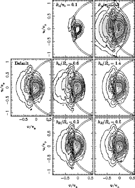
Figure 14: Velocity distribution in the $u-v$ plane after $120$ bar rotations as a function of initial conditions and using the backward integration technique. The space position is $R_{\circ}/R_{\hbox{\tiny OLR}}=1.1$ and $\varphi=25^{\circ}$ and the bar strength $F=0.10$. The left frame shows the result for the default values of the parameters, i.e. $\tilde{\sigma}_{\circ}/v_{\circ}=0.2$, $h_{\sigma}/R_{\circ}=1$ and $h_{R}/R_{\circ}=0.33$, and the other frames the results when changing only one parameter at a time to the indicated value. The velocity contours are as in Fig. 1 and the circular arcs represent the $H_{12}$ and $H_{45}$ contours.

Increasing the overall initial velocity dispersion (top frames in Fig. 14) yields a larger final velocity dispersion. Hence in this kind of simulations the particles remember the initial conditions and the action of the bar is unable to completely erase them. Also, the $u-v$ density in the Hercules-like stream is enhanced relative to the density within the main velocity mode. This is because the larger velocity dispersion lowers the peak of the latter mode, and because a larger $\tilde{\sigma}_{\circ}$ increases the average Hamiltonian value of the particles and thus the fraction of hot chaotic particles. Reducing the initial velocity dispersion scale length keeping the same velocity dispersion at $R_{\circ}$ (middle frames) renders the inner regions hotter and hence mainly increases the density of the velocity distribution at low angular momentum. To increase the relative fraction of stars in the Hercules-like stream, the most efficient way seems to start with a smaller disc scale length (bottom frames). This represents a higher initial space density of the disc in the inner regions where the particles have larger $H$-values on the average and thus again a larger fraction of hot chaotic particles which will be spread over the whole disc by the barred potential.

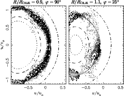
Figure 15: For two different space positions and after $120$ bar rotations, traces in the $u-v$ plane of the trajectories which were in OLR with the unperturbed rotating potential at $t=0$ (bar strength $F=0.10$). The points are colour-coded according to the angle $\alpha$ between the line joining the apocentres of the initial resonant orbit and the major axis of the vanishing bar potential: black if $|\alpha|<45^{\circ}$, light grey if $|\alpha|>70^{\circ}$, and dark grey for intermediate angles.

By changing the initial conditions, it is therefore possible to achieve a more pronounced main chaotic overdensity than in the results based on the default parameters and also to match more precisely the observed velocity dispersions in the Solar neighbourhood.

9 Resonances and stochasticity

A worthful exercise is to determine what happens to the periodic orbits which are initially in (outer) $2/1$ resonance before the growth of the bar. This is illustrated in Fig. 15, which highlights for two different space positions at $t=120t_{\rm b}$ the points in the $u-v$ plane corresponding to trajectories which were on such orbits at $t=0$. The diagrams are built by integrating backwards the trajectories passing through a Cartesian $u-v$ grid and marking all the points on this grid originating from initial orbits with $(\omega_{\phi}+2\omega_{R}-\Omega_{\rm P})/\Omega_{\rm P}<10^{-2}$. The darkness of the points reflects the angle $\alpha$ between the major axis of the initial resonant orbit and the major axis of the then vanishing bar potential, with darker points standing for smaller angles, i.e. resonant orbits with apocentre closer to the bar major axis.

At $\varphi=90^{\circ}$ and $R/R_{\hbox{\tiny OLR}}=0.9$, there is a wide region of regular orbits around most of the $2/1$ resonance curve (see Fig. 7). The trajectories with small $\alpha$’s clearly fall in the inner part of this region, while those with larger $\alpha$’s appear rather on its edge and are spread within the neighbouring chaotic regions. In addition to the regular versus chaotic phase space decoupling, the fact that the OLR curve is associated with a valley in the planar velocity distribution (see Fig. 12) is also because the phase space density in the chaotic regions bounding the regular orbit arc around this curve is forced to be a function of $H$ only, hence lowering the density on the low-$v$ side and increasing it on the other side relative to the initial densities. At $\varphi=25^{\circ}$ and $R/R_{\hbox{\tiny OLR}}=1.1$, the part of the $2/1$ resonance curve within the $u>0$ chaotic region has no nearby small-$\alpha$ points and is embedded in a broad cloud of high-$\alpha$ points.

Hence, the initial $2/1$ resonant orbits more nearly aligned with the bar major axis end into regular regions, while only those more nearly perpendicular to this axis are scattered into chaotic regions. This is consistent with the stability properties of the low-eccentricity $x_{1}(1)$ and $x_{1}^{*}(2)$ orbits in the full barred potential, which are both $2/1$ periodic orbits.

10 $N$-body models

In addition to the test particle simulations, we have also run a high-resolution $N$-body simulation whose predictions can be compared with the results of the former sections. The main difference of this simulation with respect to the previous simulations is that it is three-dimensional and completely self-consistent, i.e. with no rigid component and allowing the development of spiral arms. The description of the simulation hereafter is based on physical units in which the initial conditions provide a reasonable axisymmetric model of the present Milky Way. In these units, $R_{\hbox{\tiny OLR}}=9$ kpc at $t=2.32$ Gyr.

The simulation, also discussed in Fux (F3 (2000)), is similar to the simulations presented in Fux (F1 (1997)), starting from a bar unstable axisymmetric model including a nucleus-spheroid, a disc and a dark halo component with parameters set to $a=1$ kpc, $M_{\rm NS}=2.6\cdot 10^{10}$ M_⊙, $h_{R}=3.2$ kpc, $h_{z}=300$ pc, $M_{\rm D}=5.0\cdot 10^{10}$ M_⊙, $b=9.1$ kpc and $M_{\rm DH}=2.6\cdot 10^{11}$ M_⊙ (in the same notation as in Fux F1 (1997)). It involves $14\,299\,552$ particles of which $5\,553\,784$ belong to the disc component. The simulation uses the double polar-cylindrical grid technique described in Fux (F2 (1999)) to solve the gravitational forces, with $N_{R}\times N_{\phi}\times N_{z}=94\times 96\times 253$, $H_{z}=25$ pc and imposed reflection symmetry with respect to the plane $z=0$ and the $z$-axis. The time integrator is a leap-frog with a time step $\Delta t=0.05$ Myr. The simulation has been carried out until $t=2.65$ Gyr. The phase space coordinates have been saved every 50 Myr for all particles and every Myr for the disc particles within a fixed annulus $7.5\leq R/{\rm kpc}\leq 10.5$.

After the formation of the bar at about $1.4$ Gyr, the simulation reveals a complex velocity structure with multiple streams occuring almost everywhere in the disc. The streams, as well as the velocity dispersions, remain very time dependent, even within space regions corotating with the bar. Some mpeg movies showing the time evolution of the $u-v$ distribution for a realistic position of the Sun are available on the web at the address http://www.mso.anu.edu.au/~fux/streams.html. However, the strong time dependency is certainly partly the consequence of incomplete phase mixing as in the test particle simulations of the previous sections. Therefore, we will again average in time the $u-v$ distributions resulting from the $N$-body simulation to minimise this problem and thus focus on the average properties of these distributions.

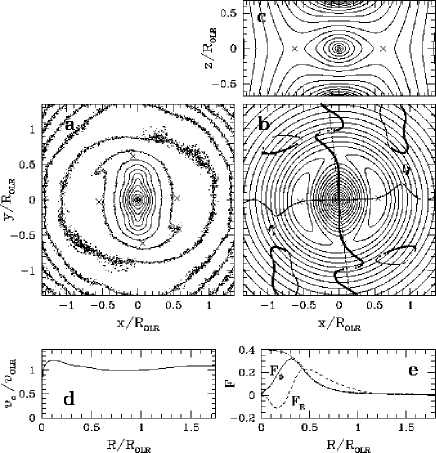
Figure 16: Some properties of the $N$-body simulation averaged over $2\leq t/{\rm Gyr}\leq 2.65$ and scaled to a time independent $R_{\hbox{\tiny OLR}}$ (see text for details). a) Face-on surface density of the luminous (disc + nucleus-spheroid) particles, with contours spaced by 0.5 magnitude. b) Effective potential in the plane $z=0$, with the spacing of the contours increasing by a factor $1.2$ as one moves from $L_{4/5}$ to lower $\Phi_{\rm eff}$ regions. The curves made of large and small dots represent respectively the azimuthal minima and maxima of $\Phi_{\rm eff}$ at local radius. In these first two frames, galactic rotation is clockwise and the crosses indicate the Lagrangian points $L_{1/2}$ and $L_{4/5}$. c) Effective potential in the vertical plane passing through the Lagrangian points $L_{1}$ and $L_{2}$ and shown by the dotted straight line in the former frame. d) Rotation curve of the axisymmetrised average model, with $v_{\hbox{\tiny OLR}}\equiv v_{\rm c}(R_{\hbox{\tiny OLR}})$. e) Radial dependence of the azimuthal and radial bar strengths $F_{\phi}$ and $F_{R}$. The unlabelled dotted curve is the azimuthal strength of the analytical barred potential given by Eq. (5) for $F=0.20$.

A complication arises from the fact that the pattern speed of the bar decreases with time due to the angular momentum the bar loses to the (live) dark halo, so that the OLR does not lie at a fixed radius anymore but moves outwards. The decrease of $\Omega_{\rm P}$ is probably not that large in real disc galaxies with a substantial gas fraction like the Milky Way, as shown by self-consistent numerical simulations with an SPH component (e.g. Friedli & Benz FB (1993)). Hence, the $u-v$ distributions at a given $R_{\circ}/R_{\hbox{\tiny OLR}}$ must be computed within space volumes comoving with $R_{\hbox{\tiny OLR}}$. We found that the evolution of the bar position angle $\vartheta(t)$ over the time interval $1.5\leq t/{\rm Gyr}\leq 2.65$ can be well fitted by an analytical function of the form:

$$\vartheta(t)=\vartheta_{\infty}-\frac{\Omega_{\circ}}{\mu}\exp{(-\mu t)},$$ (15)

where $\vartheta_{\infty}$, $\Omega_{\circ}$ and $\mu$ are the free parameters, with residuals in $\vartheta$ never exceeding $5^{\circ}$. From this we obtain $\Omega_{\rm P}(t)={\rm d}\vartheta/{\rm d}t$ and $R_{\hbox{\tiny CR}}(t)=v_{\circ}^{\prime}/\Omega_{\rm P}(t)$, where $v_{\circ}^{\prime}$ is matched so that $R_{\hbox{\tiny CR}}=[R(L_{1/2})+R(L_{4/5})]/2$ on the average. The radius of the OLR is then derived from $R_{\hbox{\tiny CR}}$ via the flat rotation curve relation, which yields a very good approximation of $R_{\hbox{\tiny OLR}}$ on the average, and represents the smoothly changing reference adopted for the distance normalisation. Because the rotation curve remains nearly flat and constant with time at intermediate $R$, no velocity scaling is required.

Figure 17: a) Characteristic diagram for the low-eccentricity $x_{1}(1)$, $x_{1}^{*}(2)$ and $x_{1}(2)$ periodic orbits in the time averaged $N$-body model. The full and dotted lines indicate stable and unstable orbits respectively, and the dashed line the zero velocity curve. $v_{\hbox{\tiny OLR}}$ is the circular velocity at the OLR in the axisymmetrised potential. All curves are interrupted at high $H$ (see text), and the $x_{1}(1)$ curve is truncated on the low-$H$ side at the outer $1/1$ resonance. b) Sequence of $x_{1}(1)$ orbits in the $x-y$ plane for the same model. The orbits are sampled at constant Hamiltonian interval and cover the whole range of the corresponding characteristic curve in the former diagram. The orientation of the bar is sketched by the shaded ellipse and its rotation is clockwise.

The time average is done over the interval $2\leq t/{\rm Gyr}\leq 2.65$ and as underlying mass distribution and potential associated with the average velocity distributions, we take those resulting from the sum of the $50$ Myr spaced output models of the simulation within the same time interval and with the mass in each model rescaled as the distances to preserve the velocity scale. The number of models added together is rather low (only 14), yielding only a crude estimate of the true average quantities, especially regarding azimuthal variations in the spiral arm regions. Figure 16 shows some properties of the resulting average model. At given radius $R$, the azimuthal and radial bar strengths $F_{\phi}(R)$ and $F_{R}(R)$ (Fig. 16e) are defined as the most extreme values over azimuth of $|A_{\phi}(R,\phi)/A_{R}^{\rm axisym}(R)|$ and $[A_{R}(R,\phi)-A_{R}^{\rm axisym}(R)]/A_{R}^{\rm axisym}(R)$ respectively, where $A_{\phi}$ and $A_{R}$ are the azimuthal and radial accelerations in the plane $z=0$ and $A_{R}^{\rm axisym}$ is the axisymmetric part of $A_{R}$. In particular, $F_{\phi}(a=R_{\hbox{\tiny CR}}/1.25)$ coincides with the definition of bar strength used in the former sections. The time averaged model has $F_{\phi}(a)\approx 0.2$, i.e. a rather strong bar. However, Buta & Block (BB (2001)) have introduced a bar strength classification in terms of a parameter $Q_{\rm b}$, corresponding here to the radial maximum of $F_{\phi}(R)$, and present galaxies with values of this parameter up to $0.65$. Our average model has $Q_{\rm b}\approx 0.325$ and thus falls only in the middle of the range covered by real galaxies.

Figure 18: Time averaged planar velocity distribution of the disc particles in the $N$-body simulation as a function of position in space and within vertical cylinders of radius $R_{\circ}/80$. The horizontal and vertical axes of the frames are $v/v_{\circ}$ and $u/v_{\circ}$ respectively, with $v_{\circ}$ being the circular velocity at local radius in the corresponding axisymmetriesed average model. The velocity contours are as in Fig. 12, as well as the $H$-contours (drawn at $z=0$), the resonance curves and the traces of the periodic orbits, which all refer to the average rotating potential. Only orbits from the $x_{1}(1)$, $x_{1}^{*}(2)$ and $x_{1}(2)$ families and within the Hamiltonian range scanned by the characteristic curves in Fig. 17a are indicated.

The disc scale length between corotation and slightly outside the OLR (Fig. 16a) has substantially increased with respect to the initial conditions, in agreement with the test particle results. The effective potential (Fig. 16b) indicates Lagrangian points which significantly lag the bar principal axes. This is the effect of the spiral arms starting at the end of the bar, which were absent in the test particle simulations and now produce a twist of the potential well. Note however that, as pointed out by Zhang (ZX (1996)), there is a phase shift between the potential and the density wells, with the former leading the latter outside the bar. The characteristic curves of the main periodic orbit families and the $x-y$ configuration of the $x_{1}(1)$ orbits in the average potential are given in Fig. 17. The characteristic curves are truncated at large $H$, where they start to bend and interfere with each other presumably as a consequence of the sharp phase change in the potential well at large radii (see Fig. 16b). The $x_{1}(1)$ orbits respond to the twisted potential well by having their major axis departing more and more from the $y$-axis as $H$ decreases, and the closed orbits of the other families share a similar response. Since the cusps of the cusped orbits now occur away from the coordinate axes, the characteristic curves no longer reach the ZVC.

The time averaged $u-v$ distributions are presented in Fig. 18. The diagrams are computed by summing the $1$ Myr spaced outputs of the simulation, yielding much more accurate time averages than for the properties based on the $50$ Myr spaced outputs, and using the same space volumes, velocity binning and smoothing procedure as for the test particle simulations. However, contrary to the latter simulations, the diagrams are based on a unique simulation and therefore the initial conditions for each diagram now scale as $R_{\hbox{\tiny OLR}}$ instead of $R_{\circ}$. Hence the pattern speed and size of the bar are not the only parameters that change for different values of $R_{\circ}/R_{\hbox{\tiny OLR}}$. In particular, the initial velocity dispersions decrease with $R$, causing a similar trend in the final velocity distributions. Diagrams have been derived at an azimuthal interval $\Delta\varphi=10^{\circ}$, but only those at $30^{\circ}$ spacing are shown.

A priori, some properties inferred from the test particle simulations seem less robust in the $N$-body simulation: the non-resonant $x_{1}(1)$ orbits are somewhat less coincident with peaks in the velocity distributions, and the resonant $x_{1}(1)$ orbits, i.e. those with traces on the $2/1$ resonance curve, are less correlated with depleted $u-v$ regions at high eccentricities. Moreover, the low angular momentum peak often lies well inside the hot orbit region even when it is still mostly associated with regular quasi-$x_{1}(2)$ orbits, as indicated by the presence of a stable low-eccentricity $x_{1}(2)$ orbit. In fact, a closer inspection reveals that the velocity distributions in the $N$-body simulation at given $R_{\circ}/R_{\hbox{\tiny OLR}}$ appear to best match those of the test particle simulations at a typically $10$% larger value of $R_{\circ}/R_{\hbox{\tiny OLR}}$. This can be explained by a delayed response of the phase space density distribution to the growing absolute OLR radius: the $u-v$ distributions do not instantaneously adjust to the moving $R_{\hbox{\tiny OLR}}$ and therefore always reflect an earlier smaller $R_{\hbox{\tiny OLR}}$ value instead of the current one. Hence the velocity distributions in Fig. 18 should virtually be shifted upwards by roughly one frame to be more consistent with the $R_{\circ}/R_{\hbox{\tiny OLR}}$ scale and the other plotted informations. Actually, the effective $R_{\hbox{\tiny OLR}}$ must be a function of the orbits.

With such a correction in mind, the $N$-body velocity distributions now share much more the same properties as in the test particle simulations. The low angular momentum mode, when purely induced by chaotic orbits as in the frame $R_{\circ}/R_{\hbox{\tiny OLR}}=1.1$ and $\varphi=30^{\circ}$ of Fig. 18, also no longer peaks outside the $H_{45}$ contour, but rather between the $H_{12}$ and the $H_{45}$ contours. The velocity distributions most resemble those of the test particle simulations with a bar strength $F=0.15$ (not shown in this paper, but see Fux 2001a ). Since $F\approx 0.20$ in our average $N$-body model, this suggests that the velocity distributions are less responsive to the bar strength in the more realistic 3D $N$-body simulation than in the 2D test particle simulations.

The symmetries found in Sect. 7 for the velocity distributions, and in particular the $u$-symmetry at $\varphi=0$ and $\varphi=90^{\circ}$, obviously break and the velocity distributions in the $N$-body model at given $\varphi$ and fixed effective radius seem to compare best with the corresponding distributions in the test particle simulations at an angle $\sim\varphi-10^{\circ}$, suggesting that the velocity distributions know about the spiral arm induced average local twist of the potential well relative to the bar major axis. While this is especially true for the more regular low-$H$ regions, the velocity distributions show no significant phase shift at all in the hot orbit region. The reason is because the hot orbits are more eccentric and therefore are sensitive to more inner features of the potential. It should be noted that in $N$-body simulations like the one presented here, spiral arms are particularly strong during about $1$ Gyr after the formation of the bar, so that the reported effects of spiral arms are probably overestimates for the Milky Way if the Galactic bar is old.

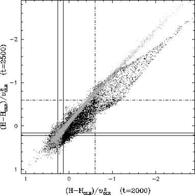
Figure 19: Comparison of the normalised Hamiltonian values of a random selection of $2\cdot 10^{5}$ disc component particles in the $N$-body simulation at times $t=2000$ and $2500$ Myr. $v_{\hbox{\tiny OLR}}$ and $H_{\hbox{\tiny OLR}}$ respectively are the velocity and Hamiltonian value of the circular orbit at the OLR of the axisymmetrised potential. The points in grey represent the particles inside the circle passing through the Lagrangian points $L_{1/2}$ at $t=2000$ Myr. These particles exist down to and beyond the smallest displayed value of $H$, as the effective potential at the central Lagrangian point is $(\Phi_{\rm eff}(L_{3})-H_{\hbox{\tiny OLR}})/v_{\hbox{\tiny OLR}}\approx-5.2$. The solid lines indicate the normalised $H_{12}$ and $H_{45}$ values and the dash-dotted lines the normalised $H$-value of the circular orbit at the outer $1/1$ resonance (in the axisymmetrised potential).

A potentially important difference of 3D models with respect to 2D models is that the effective potential a star experiences near corotation depends on its distance from the Galactic plane (see Fig. 16c). This raises the average value of the Jacobi integral required for the stars to cross the corotation radius and thus renders such a crossing more difficult. For stars on the Solar circle, the higher effective value of $H_{12}$ is not compensated by their departure from the Galactic plane or a $w$ velocity component. Indeed, in our average $N$-body model, the change of effective potential near corotation when moving from $z=0$ to $z=300$ pc is $\Delta\Phi_{\rm eff}/v_{\hbox{\tiny OLR}}^{2}\approx 0.233$ (with $v_{\hbox{\tiny OLR}}$ as defined in the caption of Fig. 17), while this change at the OLR of the axisymmetrised potential is only $0.004$, and adding a vertical velocity of $w/v_{\hbox{\tiny OLR}}=0.1$ only increases $H/v_{\hbox{\tiny OLR}}^{2}$ by $0.005$. Hence 2D models certainly exaggerate the traffic of stars on hot orbits travelling from one side of corotation to the other.

Finally, Fig. 19 shows how the value of the Hamiltonian is conserved during the $N$-body simulation. The main result is that the $H$-values at different times are much better related for bar particles than for (the dynamically defined) disc and hot particles. In particular, bar particles remain bar particles, but disc particles can easily transform into hot particles and vice versa for $(H-H_{\hbox{\tiny OLR}})/v_{\hbox{\tiny OLR}}^{2}\ga-0.2$, supporting the presumption in Sect. 7 that spiral arms may induce exchanges between regular and chaotic phase space regions in real galaxies. Near the $1/1$ resonance, the disc particles also reveal a smaller scatter of their past versus present $H$ relation. The normalised Hamiltonian (as well as the absolute non-rescaled Hamiltonian) increases on the average for the disc particles, which may be understood by the fact that the contribution of the term $-\Omega_{\rm P}^{2}R^{2}/2$ to $\Phi_{\rm eff}$ diminishes as the bar rotates slower, and decreases for the bar particles, owing to the deepening of the central potential well.

It would be interesting to investigate the evolution of the particle $H$-values in an $N$-body simulation with a bar rotating at a constant frequency, for example without including a live dark halo component, in order to disentangle the effects of the spiral arms from the effects of a decreasing pattern speed. It would be also worth to explore the diffusion of particles from regular to chaotic phase space regions and vice versa, starting with 2D $N$-body simulations in a first approach. One problem to be clarified is why the $N$-body velocity distributions look so similar to the test particle ones, despite the action of such a diffusion process. A detailed analysis of the orbital structure in 3D models remains to be done, and in particular of the properties of the vertical motion within regular and chaotic regions.

11 Models versus observations

Before concluding, we now present a selection of test particle and $N$-body velocity distributions yielding a good match to the observed one, confront the quasi-$x_{1}(2)$ orbit and chaotic orbit interpretations of the Hercules stream, paying also attention to the case of the Hyades stream, and discuss how the models could be further improved.

Beside the parameters in the initial conditions of the simulations, the free model parameters are $R_{\circ}/R_{\hbox{\tiny OLR}}$, $\varphi$, the velocity scale specified by $v_{\circ}$ (defined as the local circular velocity in the axisymmetric part $\Phi_{\circ}$ of the potential for the $N$-body simulation), which should lie between $180$ and $230$ km s^-1 (e.g. Sackett PS (1997)), and the velocity of the Sun $(v_{\rm s},u_{\rm s})$ relative to the circular orbit in $\Phi_{\circ}$. A commonly adopted velocity reference in the Solar neighbourhood is the LSR, defined as the velocity of the most nearly circular closed orbit passing through the present location of the Sun according to Binney & Merrifield (BM (1998)). This definition, which is merely an attempt to generalise the circular LSR orbit of the axisymmetric case to non-axisymmetric potentials, is not always well adapted. The most reasonable LSR orbit candidates near the OLR of a barred potential indeed are the stable low-eccentricity $x_{1}(1)$ and $x_{1}(2)$ orbits, but some space positions near the OLR circle are visited by neither of these orbits in our models (see for example $R_{\circ}/R_{\hbox{\tiny OLR}}=1.0$ and $\varphi=30^{\circ}$ in Fig. 12). However, for $R_{\circ}/R_{\hbox{\tiny OLR}}\ga 1.0$, there always exists a prominent peak of low-eccentricity quasi-$x_{1}(1)$ orbits in the model velocity distributions, which, as pointed out in Sect. 7, not necessarily coincides with the trace of the non-resonant $x_{1}(1)$ orbit when there is one. The maximum of this peak will therefore be taken as the model “LSR” and will be preferably associated to the Coma Berenices stream, which is the local maximum in the observed velocity distribution that lies closest to the heliocentric velocity of the LSR $(v,u)_{\rm LSR}\approx(-5,10)$ km s^-1 derived from the Hipparcos data (Dehnen & Binney DB (1998)).

For $R_{\circ}\ga R_{\hbox{\tiny OLR}}$, the quasi-$x_{1}(1)$ peak is always close to the circular orbit of the axisymmetrised potential, except near the OLR radius and $\varphi=90^{\circ}$ where it reaches a maximum positive $v$-offset of $\sim 0.05v_{\circ}$ for all explored bar strengths. Under the above circumstances and for realistic space positions, the azimuthal velocity of the Sun should exceed the circular velocity by $5-10$ km s^-1.

The selected model velocity distributions are displayed in Fig. 20. The distributions are derived according to the same procedures as described in Sects. 7 and 10. Frame (a) shows a case where the Hercules-like stream is induced exclusively by chaotic orbits and peaks inside the $H_{12}$ contour, illustrating the fact that chaotic modes not necessarily only occur in the hot orbit region. Here the Hyades stream coincides with a chaotic overdensity associated with a narrow and low-$H$ chaotic breach roughly along the OLR curve, i.e. an interpretation similar to the one proposed in Sect. 7 for the $u<0$ extension of the LSR mode. Frame (c) gives a case where the Hercules-like stream now falls entirely in the hot orbit region and where the Hyades stream has the same chaotic origin as in frame (a).

Frame (e), derived from the $N$-body simulation and presenting a larger velocity dispersion, provides a remarkable example of a Hercules-like stream sustained exclusively by quasi-$x_{1}(2)$ orbits. The test particle simulations develop quasi-$x_{1}(2)$ modes which cannot be as easily matched to the Hercules stream in our scaling procedure, generally falling right between this stream and the Hyades stream. This can be explained by the different local slope of the circular velocity $v_{\rm c}$ in the $N$-body and the test particle models. As explained by D2000 in terms of orbital frequencies, the separation between the quasi-$x_{1}(1)$ and the quasi-$x_{1}(2)$ modes increases with ${\rm d}v_{\rm c}/{\rm d}R(R_{\circ})$. Since the average $N$-body model has a slightly raising rotation curve near the OLR radius (Fig. 16d), its circular velocity gradient is larger than for the flat rotation curve test particle simulations and thus the quasi-$x_{1}(2)$ mode is found at higher asymmetric drift relative to the quasi-$x_{1}(1)$ mode. However, the fact that observations support a rather gently declining rotation curve at $R_{\circ}$ and that a large inclination angle of the bar is needed ($\varphi\ga 40^{\circ}$ for $R_{\circ}>R_{\hbox{\tiny OLR}}$) are arguments against the quasi-$x_{1}(2)$ interpretation of the Hercules stream. On the other hand, the displacement of the quasi-$x_{1}(2)$ peak towards the $H_{12}$ contour with increasing integration time mentioned in Sect. 7 for $F=0.10$ and $R_{\circ}\approx R_{\hbox{\tiny OLR}}$ may reinforce this interpretation.

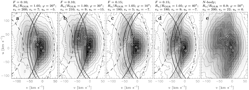
Figure 20: Selection of scaled velocity distributions from the test particle (frame a to d) and $N$-body (frame e) simulations, with the various parameters indicated on the top of the frames and the velocity origin at the adopted Solar motion. The velocity window and the velocity contours are the same as in Fig. 1. The filled circles represent the mean velocities of the streams listed in Table LABEL:stream, excluding the Arcturus stream. All distributions from the test particle simulations are time averages over $55\leq t/t_{\rm b}\leq 65$. The $H$-contours and the resonance curves are as in Fig. 7 and are not plotted for the $N$-body model because of the time delay problem discussed in Sect. 10.

Frame (d) is an example with two distinct low angular momentum peaks, the most negative $v$ one being related to chaotic hot orbits and the other one to quasi-$x_{1}(2)$ orbits. It would be interesting to check whether a sufficiently negative ${\rm d}v_{\rm c}/{\rm d}R(R_{\circ})$ is able to shift the quasi-$x_{1}(2)$ mode more towards the true location of the Hyades stream and thus yield a model velocity distribution with a better overall match to the observed one. Note that the chaotic orbit mode will not necessarily be shifted as the quasi-$x_{1}(2)$ mode, because its location in the $u-v$ plane does not actually depend on the local slope of the circular velocity, but rather on the difference of $\Phi_{\rm eff}$ between the current space position and the Lagrangian point $L_{1/2}$, which determines the $u-v$ location of the $H_{12}$ contour. Finally, frame (b) displays a surprising case where the velocity distribution in the quasi-$x_{1}(2)$ region of the $u-v$ plane (see Fig. 9) seems to have split into two peaks coinciding well with the locations of the Hercules and Hyades streams, i.e. both these streams have a quasi-$x_{1}(2)$ origin. However, this is likely to be a transitory situation resulting from the unachieved phase mixing near $R_{\circ}=R_{\hbox{\tiny OLR}}$ (see Sect. 7).

These examples illustrate the variety of possible interpretations for the Hercules and Hyades streams, and it is very hard at this stage to decide with certainty which one is the most appropriate. The splitting of the LSR mode into the Pleiades, Coma Berenices, Sirius and other streams is probably not related to the bar itself and has a more local origin, like for instance the effect of time dependent spiral arms.

12 Conclusion

The Galactic bar induces a characteristic splitting of the disc phase space into regular and chaotic orbit regions, with the latter regions owing only to the non-axisymmetric part of the potential in the limit of no vertical motion. In this paper, we have isolated these two kind of regions, as well as the quasi-periodic orbit sub-regions inside the regular regions associated with the stable $x_{1}(1)$ and $x_{1}(2)$ periodic orbits respectively, within the same analytical 2D rotating barred potential with flat azimuthally averaged rotation curve as in D2000. We then have run test particle simulations in this potential and a more realistic self-consistent 3D $N$-body simulation to find out how the disc distribution function outside the bar region relates to such a phase space splitting and in particular how chaos may explain features in the Solar neighbourhood stellar kinematics like the Hercules stream.

Beside the bar strength, the regular versus chaotic splitting of phase space, investigated via the largest Liapunov exponent, is mainly determined by the value of the Hamiltonian $H$ (or Jacobi’s integral) and by the bar related resonances. In two dimensions and at fixed space position, the constant-$H$ contours in the galactocentric $u-v$ velocity plane are circles centred on $(v,u)=(R_{\circ}\Omega_{\rm P},0)$ and of radius $\sqrt{2(H-\Phi_{\rm eff}^{\circ})}$, where $R_{\circ}$ is the galactocentric distance, $\Omega_{\rm P}$ the rotation frequency of the bar and $\Phi_{\rm eff}^{\circ}$ the local effective potential. The fraction of chaotic orbits increases with $H$ and there is a sharp average transition from regular to chaotic behaviour in the $u-v$ plane when crossing the contour corresponding to the effective potential at the saddle Lagrangian points, $H_{12}\equiv\Phi_{\rm eff}(L_{1/2})$, which generally intersects the $v$-axis at lower velocity than the circular orbit in the axisymmetric part of the potential. At $H<H_{12}$, the orbits are rather regular, while at $H>H_{12}$, which defines the category of hot orbits susceptible to cross the corotation radius, they are rather chaotic.

The resonances, on the other hand, generate an alternation of regular and chaotic orbit arcs in the velocity plane which, contrary to the low-$v$ part of the $H$-contours, are opened towards lower angular momentum. At bar inclination angles $\varphi=0$ and $\varphi=90^{\circ}$, the maxima or minima of these stochasticity waves are in phase with the resonance curves derived from the axisymmetric limit and the arcs are symmetric in $u$, reflecting the four-fold symmetry of the potential. At intermediate angles, these extrema become offset with respect to the resonance curves and the $u$-symmetry breaks. In particular, at $R\ga R_{\hbox{\tiny OLR}}$ and $\varphi\sim 30^{\circ}$, a prominent regular region of eccentric quasi-$x_{1}(1)$ orbits extends well within the hot orbit region at $u\la 0$, while the $u>0$ counterpart of the OLR curve is surrounded by a wide chaotic region consistent with the location of the Hercules stream.

For a moderate bar strength ($F=0.10$), the low-eccentricity and non-resonant quasi-$x_{1}(2)$ orbit regions exist only for $R/R_{\hbox{\tiny OLR}}\la 1.1$ and over an angle range around $\varphi=90^{\circ}$ increasing towards smaller $R$. There is no such region near the default position considered in D2000, i.e. $R/R_{\hbox{\tiny OLR}}\approx 1.1$ and $\varphi=25^{\circ}$, compromising the quasi-$x_{1}(2)$ orbit interpretation given by Dehnen for the Hercules-like mode occuring in his simulations at the most realistic positions of the Sun relative to the bar.

The test particle simulations, started from axisymmetric initial conditions and progressively exposed to the full rotating barred potential, reveal a decoupled evolution of the disc distribution function within the regular and chaotic phase space regions. In the regular regions, the phase space density after phase mixing is roughly the same as the initial one, whereas in the chaotic regions, the particles quickly evolve towards a uniform population of the easily available phase space volume via chaotic mixing, resulting in a substantial density re-adjustment. Because the space region within corotation represents a large initial reservoir of hot chaotic orbit particles which are spread throughout the disc by this process, yielding a net outward migration of such particles, the chaotic regions in the $u-v$ plane outside corotation become more heavily crowded than the regular regions at $H\ga H_{12}$. In particular, the wide and predominantly $u>0$ chaotic region mentioned above for realistic space positions of the Sun appears as an overdensity in the $u-v$ distribution, providing a coherent interpretation of the Hercules stream and explaining the $u>0$ property of this stream. According to this interpretation, the Hercules stream involves stars on essentially chaotic orbits which are forced to avoid the regular $x_{1}(1)$ region at negative $u$.

The time averaged disc $u-v$ velocity distributions inferred from the $N$-body simulation are remarkably similar to those of the test particle simulations, despite the action of the transient spiral arms which allows at least some of the particles to diffuse from the regular to the chaotic regions and vice versa. At low eccentricity, the orbits are less sensitive to the inner features of the potential and the azimuthal properties of the velocity distributions essentially align with the average local phase shift of the potential well relative to the bar major axis induced by the spiral arms.

The velocity distributions may be very time dependent if for instance the bar has formed recently, because of the phase mixing occuring in the disc during at least $\sim 10$ bar rotations after the growth of the bar according to the test particle simulations. The $u-v$ distributions in the $N$-body simulation at fixed space position relative to the bar also display a strong temporal behaviour (see the mpeg movies at http://www.mso.anu.edu.au/~fux/streams.html), as expected from the presence of the transient spiral waves. However, since the simulation has been run for only about $1.25$ Gyr after the formation of the bar, phase mixing is still operating in the disc component, rendering difficult to disentangle from it the individual effects of such waves. The $N$-body simulation also gives some insight on the consequences of evolving bar parameters: the slowly decreasing pattern speed of the bar mainly introduces a delayed response of the disc distribution function to the outward moving resonances, so that the velocity distributions at a given time rather reflect a higher value of $R/R_{\hbox{\tiny OLR}}$ than the true instantaneous one when compared with the constant $\Omega_{\rm P}$ test particle simulations. For completeness, one should mention that other perturbations than the bar and the spiral arms may provide alternative explanations of the local stellar streams, like for example the interactions of the Milky Way with its satellite companions.

Finally, the process of chaotic mixing, combined with the possible stellar exchanges between the regular and chaotic phase space regions resulting from the diffusion of stars by transient spiral arms or molecular clouds, may provide an new and efficient way of heating galactic discs which remains to be explored.

- (1) Alcock C., Allsman R.A., Alves D.R., et al. 2000, ApJ, 541, 734
- (2) Asiain R., Figueras F., Torra J., & Chen B. 1999, A&A, 341, 427
- (3) Athanassoula E., Bienaymé O., Martinet L., & Pfenniger D. 1983, A&A, 127, 349
- (4) Benettin G., Galgani L., & Strelcyn J.M. 1976, Phys. Rev., A14, 2338
- (5) Binney J., & Merrifield M. 1998, in Galactic Astronomy, ed. J.P. Ostriker, & D.N. Spergel (Princeton Univ. Press, New Jersey), p. 536
- (6) Binney J., & Tremaine S. 1987, in Galactic Dynamics, ed. J.P. Ostriker (Princeton Univ. Press, New Jersey), p. 146
- (7) Binney J., Gerhard O.E., Stark A.A., Bally J., & Uchida K.I. 1991, MNRAS, 252, 210
- (8) Binney J., Gerhard O., & Spergel D. 1997, MNRAS, 288, 365
- (9) Binney J.J., Dehnen W., Houk N., Murray C.A., & Penston M.J. 1997, in Hipparcos–Venice’97, ESA SP-402, 473
- (10) Blitz L., & Spergel D.N. 1991, ApJ, 379, 631
- (11) Buta R., & Block D.L. 2001, ApJ, 550, 243
- (12) Caloi V., Cardini D., D’Antona F., et al. 1999, A&A, 351, 925
- (13) Chereul E., Crézé M., & Bienaymé O. 1998, A&A, 340, 384
- (14) Contopoulos G., & Barbanis B. 1989, A&A, 222, 329
- (15) Contopoulos G., & Grosbol P. 1989, A&AR, 1, 261
- (16) Dehnen W. 1998, AJ, 115, 2384
- (17) Dehnen W. 1999a, AJ, 118, 1201
- (18) Dehnen W. 1999b, ApJ, 524, L35
- (19) Dehnen W. 2000, AJ, 119, 800 (D2000)
- (20) Dehnen W., & Binney J.J. 1998, MNRAS, 298, 387
- (21) Eggen O.J. 1966, Royal Obs. Bulletins, 125, 149
- (22) Elmegreen B. 1996, in Proc. IAU Coll. 157, ASP Conf. Ser. 91, Barred Galaxies, ed. R. Buta, D.A. Crocker, & B.G. Elmegreen, 197
- (23) Englmaier P., & Gerhard O. 1999, MNRAS, 304, 512
- (24) Feast M.W., & Whitelock P.A. 2000, MNRAS, 317, 460
- (25) Fehlberg E. 1968, NASA Technical Report TR R-287
- (26) Friedli D., & Benz W. 1993, A&A, 268, 65
- (27) Fux R. 1997, A&A, 327, 983
- (28) Fux R. 1999, A&A, 345, 787
- (29) Fux R. 2000, in ASP Conf. Ser. 197, Dynamics of Galaxies: From the Early Universe to the Present, ed. F. Combes, G.A. Mamon, & V. Charmandaris, 27
- (30) Fux R. 2001a, in ASP Conf. Ser. 228, Dynamics of Star Clusters and the Milky Way, ed. S. Deiters, B. Fuchs, A. Just, R. Spurzem, & R. Wielen, 283 (astro-ph/0007363)
- (31) Fux R. 2001b, in Stellar Dynamics: from Classical to Modern, ed. L.P. Ossipkov, & I.I. Nikiforov (Saint-Petersburg Univ. Press), 209
- (32) Fux R., Martinet L., & Pfenniger D. 1995, in The Formation of the Milky Way, ed. E.J. Alfaro, & A.J. Delgado (Cambridge Univ. Press), 243
- (33) Gerhard O.E. 1999, in ASP Conf. Ser. 182, Galaxy Dynamics, ed. D. Merritt, J.A. Sellwood, & M. Valluri, 307
- (34) Gilmore G., Wyse R.F.G., & Kuijken K. 1989, ARA&A, 27, 555
- (35) Gyuk G. 1999, ApJ, 510, 205
- (36) Kalnajs A. 1991, in Dynamics of Disc Galaxies, ed. B. Sundelius (Göteborg University), 323
- (37) Kandrup H.E. 2001, in Stellar Dynamics: from Classical to Modern, ed. L.P. Ossipkov, & I.I. Nikiforov (Saint-Petersburg Univ. Press), 213 (astro-ph/0010325)
- (38) Kaufmann D.E., & Contopoulos G. 1996, A&A, 309, 381
- (39) Kuijken K. 1997, ApJ, 486, L19
- (40) Martinet L., & Raboud D. 1999, Ap&SS, 265, 371
- (41) Mayor M. 1972, A&A, 18, 97
- (42) Nakada Y., Deguchi S., Hashimoto O., et al. 1991, Nat, 353, 140
- (43) Nikolaev S., & Weinberg M.D. 1997, ApJ, 487, 885
- (44) Oseledec V.I. 1968, Trans. Moscow Math. Soc., 19, 197
- (45) Paczynski B., Stanek K.Z., Udalski A., et al. 1994, ApJ, 435, L113
- (46) Pfenniger D., & Friedli D. 1991, A&A, 252, 75
- (47) Raboud D., Grenon M., Martinet L., Fux R., & Udry S. 1998, A&A, 335, L61
- (48) Sackett P.D. 1997, ApJ, 483, 103
- (49) Sellwood J.A., & Wilkinson A. 1993, Rep. Prog. Phys., 56, 173
- (50) Sevenster M., Saha P., Valls-Gabaud D., & Fux R. 1999, MNRAS, 307, 584
- (51) Shu F.H. 1969, ApJ, 158, 505
- (52) Skuljan J., Hearnshaw J.B., & Cottrell P.L. 1999, MNRAS, 308, 731
- (53) Sparke L.S., & Sellwood J.A. 1987, MNRAS, 225, 653
- (54) Stanek K.Z., Udalski A., Szymanski M., et al. 1997, ApJ, 477, 163
- (55) Udry S., & Pfenniger D. 1988, A&A, 198, 135
- (56) Weiner B.J., & Sellwood J.A. 1999, ApJ, 524, 112
- (57) Woolley R., Epps E.A., Penston M.J., & Pocock S.B. 1970, Royal Obs. Annals, 5, 1
- (58) Zhang X. 1996, ApJ, 457, 125