astro-ph/0105397

CERN–TH/2001-129

UMN–TH–2005/01, TPI–MINN–01/21

Primordial Nucleosynthesis with CMB Inputs:
Probing the Early Universe and Light Element Astrophysics

Richard H. Cyburt¹, Brian D. Fields², and Keith A. Olive^{3,4 1}Department of Physics
University of Illinois, Urbana, IL 61801, USA
²Center for Theoretical Astrophysics, Department of Astronomy
University of Illinois, Urbana, IL 61801, USA
³TH Division, CERN, Geneva, Switzerland
⁴Theoretical Physics Institute, School of Physics and Astronomy,
University of Minnesota, Minneapolis, MN 55455, USA

Abstract

Cosmic microwave background (CMB) determinations of the baryon-to-photon ratio $\eta\propto\Omega_{\rm baryon}h^{2}$ will remove the last free parameter from (standard) big bang nucleosynthesis (BBN) calculations. This will make BBN a much sharper probe of early universe physics, for example, greatly refining the BBN measurement of the effective number of light neutrino species, $N_{\rm\nu,eff}$. We show how the CMB can improve this limit, given current light element data. Moreover, it will become possible to constrain $N_{\rm\nu,eff}$ independent of ⁴He, by using other elements, notably deuterium; this will allow for sharper limits and tests of systematics. For example, a 3% measurement of $\eta$, together with a 10% (3%) measurement of primordial D/H, can measure $N_{\rm\nu,eff}$ to a $95\%$ confidence level of $\sigma_{95\%}(\mbox{$N_{\rm\nu,eff}$})=1.8$ (1.0) if  $\eta\sim 6.0\times 10^{-10}$. If instead, one adopts the standard model value $\mbox{$N_{\rm\nu,eff}$}=3$, then one can use $\eta$ (and its uncertainty) from the CMB to make accurate predictions for the primordial abundances. These determinations can in turn become key inputs in the nucleosynthesis history (chemical evolution) of galaxies thereby placing constraints on such models.

May 2001

1 Introduction

Cosmology is currently undergoing a revolution spurred by a host of new precision observations. A key element in this revolution is the measurement of the anisotropy in the cosmic microwave background (CMB) at small angular scales [1] - [4]. In principle, an accurate determination of the CMB anisotropy allows for the precision measurement of cosmological parameters, including a very accurate determination of the baryon density $\rho_{\rm B}\propto\Omega_{\rm B}h^{2}$. Because the present mean temperature of the CMB is extremely well-measured, one can then infer the baryon-to-photon ratio $\eta=n_{\rm B}/n_{\gamma}$, via $\eta_{10}=\eta\times\!10^{10}=274\Omega_{\rm B}h^{2}$.

To date, big bang nucleosynthesis (BBN) provides the best measure of $\eta$, as this is the only free parameter of standard BBN (assuming the number of neutrino species $\mbox{$N_{\rm\nu,eff}$}=3$, as in the standard electroweak model; see below). The CMB anisotropies thus independently test the BBN prediction [5]. Initial measurements of the CMB anisotropy already allow for the first tests of CMB-BBN consistency. At present, the predicted BBN baryon densities agree to an uncanny level with the most recent CMB results [3, 4]. The recent result from DASI [3] indicates that $\Omega_{B}h^{2}=0.022^{+0.004}_{-0.003}$, while that of BOOMERanG-98 [4], $\Omega_{B}h^{2}=0.021^{+0.004}_{-0.003}$ (using 1$\sigma$ errors) which should be compared to the BBN predictions, $\Omega_{B}h^{2}=0.021$ with a 95% CL range of 0.018 – 0.027, based only on D/H in high redshift quasar absorption systems [6]. These determinations are higher than the value $\Omega_{B}h^{2}=0.009$ (0.006 – 0.017 95% CL) based on ⁴He and ⁷Li [7]. However, the measurements of the Cosmic Background Imager (CBI; Padin et al. [2]) at smaller angular scales (higher multipoles) agree with lower BBN predictions and claims a maximum likelihood value for $\Omega_{B}h^{2}=0.009$ (albeit with a large uncertainty). We also note that in the DASI analysis [3], values of $\Omega_{B}h^{2}<0.01$ were not considered, and therefore we consider their result an upper limit to the baryon density.

In this paper we anticipate the impact on BBN of future high-precision CMB experiments. We begin with a summary (§2) of BBN analysis. In §3 we examine the test of cosmology which will come from comparing the BBN and CMB determinations of the cosmic baryon density. In §4 we describe and quantify the enhanced ability to probe the early universe, and quantify the precision with which primordial abundances can be predicted and thereby constrain various astrophysical processes. The impact of improvements in the observed abundances and theoretical inputs are discussed in §5, and discussion and conclusions appear in §6.

2 Formalism and Strategy

As is well known, BBN is sensitive to physics at the epoch $t\sim 1$ sec, $T\sim 1$ MeV. For a given $\eta$, the light element abundances are sensitive to the cosmic expansion rate $H$ at this epoch, which is given by the Friedmann equation $H^{2}=8\pi G\rho_{\rm rel}\sim g_{*}T^{4}/m_{\rm pl}^{2}$, and is sensitive (through $g_{*}$) to the number of relativistic degrees of freedom in equilibrium. Thus the observed primordial abundances measure the number of relativistic species at the epoch of BBN, usually expressed in terms of the effective or equivalent number of neutrino species $N_{\rm\nu,eff}$ [8]. By standard BBN we mean that $\eta$ is homogeneous and the number of massless species of neutrinos, $\mbox{$N_{\rm\nu,eff}$}=3$. In this case, BBN has only one free parameter, $\eta$. We will for now, however, relax the assumption of exactly three light neutrino species. In this case, BBN becomes a two-parameter theory, with light element abundance predictions a function of $\eta$ and $N_{\rm\nu,eff}$.

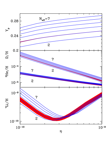
Figure 1: BBN abundance predictions as a function of the baryon-to-photon ratio $\eta$, for $\mbox{$N_{\rm\nu,eff}$}=2$ to 7. The bands show the $1\sigma$ error bars. Note that for the isotopes other than Li, the error bands are comparable in width to the thickness of the abundance curve shown. All bands are centered on $\mbox{$N_{\rm\nu,eff}$}=3$.

In Figure 1, we plot the primordial abundances as a function of $\eta$ for a range of $N_{\rm\nu,eff}$ from 2 to 7. We see the usual offset in ⁴He, but also note the shifts in the other elements, particularly D, and also Li over some ranges in $\eta$. Because of these variations, one is not restricted to only ⁴He in testing $N_{\rm\nu,eff}$ and particle physics.

To quantify the predictions of BBN and their consistency with the CMB, we adopt a likelihood analysis in the usual manner [9]. Using BBN theory in Monte Carlo simulations, one computes mean abundances, usually quantified as $y_{{\rm th},i}=(Y_{p},{\rm D/H},{\rm\mbox{${}^{3}${\rm He}}/H},{\rm\mbox{${}^{7}${\rm Li}}/H})$, and the theory error matrix $C_{ij}$ as functions of $\eta$ and $N_{\rm\nu,eff}$. Using these, one can construct a likelihood distribution ${\cal L}_{\rm BBN}(\eta,\mbox{$N_{\rm\nu,eff}$};\vec{y})$. One finds that the propagated errors are well approximated by gaussians, in which case we can write

$${\cal L}_{\rm BBN}(\eta,\mbox{$N_{\rm\nu,eff}$};\vec{y})=\frac{1}{\sqrt{(2\pi)^{N}|C|}}\ \exp\left[-\frac{1}{2}(\vec{y}-\vec{y}_{\rm th})^{T}C^{-1}(\vec{y}-\vec{y}_{\rm th})\right]$$ (1)

This function contains all of the statistical information about abundance predictions and their correlations at each $(\eta,\mbox{$N_{\rm\nu,eff}$})$ pair.

Eq. (1) can be used as follows:

1. Testing BBN: Typically, concordance is sought for the $\mbox{$N_{\rm\nu,eff}$}=3$ case [10]. Each value of the single free parameter $\eta$ predicts four light nuclide abundances. Thus the theory is overconstrained if two or more primordial abundances are known. With these abundances as inputs, it is possible to determine if the theory is consistent with the data for any range of $\eta$, and if so, one can determine the allowed $\eta$ range; this is the standard BBN prediction.

2. Probing the Early Universe: In this extension to case (1), one allows for $\mbox{$N_{\rm\nu,eff}$}\neq 3$, and uses two or more abundances simultaneously to constrain $\eta$ and $N_{\rm\nu,eff}$. One therefore derives information about particle physics in the early universe, via $N_{\rm\nu,eff}$, as well as (somewhat looser) limits on $\eta$ [9, 11, 12]. This approach can be made quantitative by convolving the likelihood in eq. (1) with an observational likelihood function ${\cal L}_{\rm OBS}(\vec{y})$

   $${\cal L}_{\rm OBS-BBN}(\eta,\mbox{$N_{\rm\nu,eff}$})=\int{\rm d}\vec{y}\ {\cal L}_{\rm BBN}(\eta,\vec{y},\mbox{$N_{\rm\nu,eff}$})\ {\cal L}_{\rm OBS}(\vec{y})$$ (2)

3. Predicting Light Element Abundances. Because the theory is overdetermined, one can use eq. (1) as a way to combine one set of abundances to determine $\eta$ (typically for $\mbox{$N_{\rm\nu,eff}$}=3$) while simultaneously predicting the remaining abundances. This procedure is less common, but has been used [13] to predict Li depletion given a ⁴He and D, or to predict D astration given Li and ⁴He.

With the advent of the CMB measurements of $\eta$, we can take a different approach to BBN. Namely, the CMB anisotropy measurements are strongly sensitive to $\eta$ and thus independently measure this parameter. The expected precision of MAP is $\sigma_{\eta}/\eta\mathrel{\raise 1.29167pt\hbox{$<$\kern-7.5pt\lower 4.30554pt\hbox{$\sim$}}}10\%$ while Planck should improve this to $\mathrel{\raise 1.29167pt\hbox{$<$\kern-7.5pt\lower 4.30554pt\hbox{$\sim$}}}3\%$ [14]. In fact, the CMB anisotropies are also weakly sensitive to the value of $N_{\rm\nu,eff}$, primarily via the early integrated Sachs-Wolfe effect. Thus, the CMB measurements will produce a likelihood of the form ${\cal L}_{\rm CMB}(\eta,\mbox{$N_{\rm\nu,eff}$})$. In practice, the CMB sensitivity to $N_{\rm\nu,eff}$ is significantly weaker than that of BBN. The current CMB limits are $\mbox{$N_{\rm\nu,eff}$}\mathrel{\raise 1.29167pt\hbox{$<$\kern-7.5pt\lower 4.30554pt\hbox{$\sim$}}}17$ (95% CL) [16], and are very sensitive to the assumed priors [17]. Thus, to simplify the following discussion, we will ignore the CMB dependence on $N_{\rm\nu,eff}$. We thus write the CMB distribution as ${\cal L}_{\rm CMB}(\eta)$, and the convolution of this with BBN theory

$${\cal L}_{\rm CMB-BBN}(\vec{y},\mbox{$N_{\rm\nu,eff}$})=\int{\rm d}\eta\ {\cal L}_{\rm BBN}(\eta,\vec{y},\mbox{$N_{\rm\nu,eff}$})\ {\cal L}_{\rm CMB}(\eta)$$ (3)

This expression gives the relative likelihoods of the primordial abundances as a function of the CMB-selected $\eta$. This will select the allowed ranges in the abundances and in $N_{\rm\nu,eff}$, and is the starting point for our analysis.

Figure 2 illustrates the combined likelihoods ${\cal L}_{\rm CMB-BBN}$ (projected on the $\eta-\mbox{$N_{\rm\nu,eff}$}$ plane) one may expect using eq. (3) and assuming a CMB determination of

$$\eta_{10}=5.80\pm 0.58\ \ \mbox{(expected {\em MAP} error)}$$ (4)

i.e., to a conservative 10% accuracy, based on the “low” deuterium observations [6]. For simplicity we have used a gaussian distribution, with a mean and standard deviation as given in eq. (4). For each element, the likelihood forms a “ridge” in the abundance–$N_{\rm\nu,eff}$ plane, tracing the curve $y_{i,{\rm max}}(\mbox{$N_{\rm\nu,eff}$})=y_{i}(\hat{\eta},\mbox{$N_{\rm\nu,eff}$})$ at the fixed $\hat{\eta}$ we have chosen. While the dependence on $N_{\rm\nu,eff}$ is not dramatic for any of the elements, the variation does exceed the width of the ridge for ⁴He, D, and ⁷Li. This sensitivity will open the possibility for D and ⁷Li to probe $N_{\rm\nu,eff}$. We do not show ³He, as these contours appear as nearly vertical lines. Note that a feature not apparent from these figures is the fact that the predicted light element abundances are correlated for a given $N_{\rm\nu,eff}$; these correlations are essential to include when combining information from predictions for multiple elements.

The combined likelihood distribution of course varies strongly with $\eta$, and so in Figure 3 we illustrate ${\cal L}_{\rm CMB-BBN}$ for

$$\eta_{10}=2.40\pm 0.24\ \ \mbox{(expected {\em MAP} error)}$$ (5)

again, a 10% measurement, this time at the value favored by ⁴He, ⁷Li, and the higher D observation [7] (and by CBI [2]). Note that at this lower value of $\eta$, D and Li show a slightly reduced sensitivity to $N_{\rm\nu,eff}$, making these elements somewhat weaker probes of this parameter.

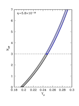
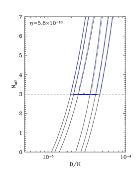
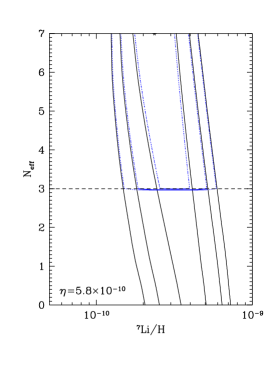
Figure 2: The likelihood distribution of eq. (3) illustrated in its $y_{i}-\mbox{$N_{\rm\nu,eff}$}$ projections. Contours show 68%, 95%, and 99% confidence levels, and the peak likelihood is displayed as a star. Solid curves are for the prior $0\leq\mbox{$N_{\rm\nu,eff}$}\leq 7$; dotted curves are for $3\leq\mbox{$N_{\rm\nu,eff}$}\leq 7$. We assume a CMB distribution in $\eta$ which is gaussian with $\eta_{10}=5.8\pm 0.58$, i.e., the expected MAP error. The departure from vertical in the peaks is a measure of the ability to constrain $N_{\rm\nu,eff}$; we see that this is the strongest for ⁴He, but is possible to a lesser extent for D and ⁷Li.

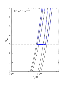
Figure 3: As in figure 2, with ${\eta}_{10}=2.4\pm 0.24$. Note the change in sensitivity to $N_{\rm\nu,eff}$.

3 Testing BBN and Cosmology

The procedure to test BBN is conceptually simple, but the details of this crucial test are important. For BBN, the difficulties stem from systematic uncertainties in the observational inference of abundances, and in the correction for post-BBN processing (chemical evolution) of the light elements prior to the epoch at which they are observed. Let us comment briefly on each of these in turn.

The ⁴He data relevant for BBN comes from observations of ⁴He in low metallicity extragalactic H II regions. A correlation is found between the ⁴He abundance and metallicity, and the primordial abundance is extracted by extrapolating the available data to zero metallicity. Because of the large number of very low metallicity observations, this extrapolation is very sound statistically and yields an error of only 0.002 (i.e. of only 1%) in Y_p. However, the method of analysis leads to a much larger uncertainty as can be seen by the various results in the literature: $0.238\pm 0.002$ [18]; $0.244\pm 0.002$ [19]; $0.234\pm 0.003$ [20]. In addition, a recent detailed examination of the systematic uncertainties in the ⁴He abundance determination showed that literature ⁴He abundances typically under-estimated the true errors by about a factor of 2 [21]. The reason for the enhanced error determinations is a degeneracy among the physical parameters (electron density, optical depth, and underlying stellar absorption) which can yield equivalent results. Without new data or a reanalysis of the existing data, it is difficult to ascribe a definite uncertainty to the ⁴He abundance at this time. For lack of a better number we will take our default value as

$$Y_{p}=0.238\pm 0.002\pm 0.005$$ (6)

As in the case of ⁴He, there is a considerable body of data on ⁷Li from observations of hot halo dwarf stars. Recent high precision studies of Li abundances in halo stars have confirmed the existence of a plateau which signifies a primordial origin [22]. Ryan et al. [23] inferred a primordial Li abundance of

$$\mbox{${}^{7}${\rm Li}}/{\rm H}=(1.23^{+0.68}_{-0.32})\times 10^{-10}$$ (7)

which includes a small correction for Galactic production which lowers ⁷Li/H compared to taking the mean value over a range of metallicity. In contrast to the downward correction due to post big bang production of Li, there is a potential for an upward correction due to depletion. Here, we note only that the data do not show any dispersion (beyond that expected by observational uncertainty). In this event, there remains little room for altering the ⁷Li abundance significantly.

The observational status of primordial D is very promising if somewhat complicated. Deuterium has been detected in several high-redshift quasar absorption line systems. It is expected that these systems still retain their original, primordial deuterium, unaffected by any significant stellar nucleosynthesis. At present, however, the determinations of D/H in different absorption systems show considerable scatter. The result for D/H already used above is [6]

$${\rm D/H}=(3.0\pm 0.4)\times 10^{-5}$$ (8)

and is based on three determinations: D/H = $(3.3\pm 0.3)\times 10^{-5}$, $(4.0\pm 0.7)\times 10^{-5}$, and $(2.5\pm 0.2)\times 10^{-5}$. O’Meara et al.  [6] note, however, that $\chi^{2}_{\nu}=7.1$ for the 3 combined D/H measurements (i.e., $\nu=2$), and interpret this as a likely indication that the errors have been underestimated. There are in addition two other determinations: D/H = $(2.25\pm 0.65)\times 10^{-5}$ [24] and $(1.65\pm 0.35)\times 10^{-5}$ [25]. At the very least all of these measurements represents lower limits to the primordial abundance.

On the CMB side, the key issue is the influence of a host of parameters on the anisotropy power spectrum. That is, individual features in the power spectrum, such as peak heights and positions, do depend on multiple parameters, and thus the measurement of a few features can leave ambiguities in the inferred cosmology. Fortunately, different features in the power spectrum depend differently on the cosmological parameters, so that a sufficiently precise measurement with sufficient angular coverage will be able to break the degeneracy represented by any one feature. Such precise measurements will be provided by the space-based missions MAP and Planck. For the rest of the paper, we will assume the existence of such measurements and thus an unambiguous determination of ${\cal L}_{\rm CMB}(\eta)$, and examine the impact of such a measurement on BBN.

4 BBN After CMB Concordance

We now quantitatively explore the predictive power of BBN with $\eta$ given by the CMB fluctuations. The BBN predictions we use, and their derivation from Monte Carlo calculations, are described in detail in [7].

BBN neutrino counting will benefit significantly from the CMB revolution. To date, BBN limits on $N_{\rm\nu,eff}$ require an accurate ⁴He abundance (to fix the neutrino number) and a good measure of at least one more abundance (to fix $\eta$). A precise determination of $\eta$ from the CMB anisotropy opens up other strategies. One no longer need use light elements to fix $\eta$, and thus all abundances are available to constrain $N_{\rm\nu,eff}$.

Abundance observations fix the distributions ${\cal L}_{i}^{\rm obs}(y_{i})$. We can convolve these with eq. 3 to obtain

$${\cal L}_{i\cdots\ell}(\mbox{$N_{\rm\nu,eff}$})=\int{\rm d}y_{i}\,\cdots\,{\rm d}y_{\ell}\ {\cal L}_{\rm CMB-BBN}(\vec{y},\mbox{$N_{\rm\nu,eff}$})\ {\cal L}_{i}(y_{i})\cdots{\cal L}_{\ell}(y_{\ell})$$ (9)

a distribution for $N_{\rm\nu,eff}$. That is, for a given nuclide, the distribution in $N_{\rm\nu,eff}$ is given by the vertical region in Figure 2 or 3 determined by the horizontal extent of the abundance measurement. Of course, combining abundance determinations sharpens the limits on $N_{\rm\nu,eff}$. One could then predict with great accuracy the abundances for any elements not used for this analysis.

As expected, the ⁴He abundance shows the most sensitivity to $N_{\rm\nu,eff}$. Figure 4a illustrates the power of such an analysis in light of CMB data. The curves show the resultant likelihood function for CMB measurements of increasing accuracy (30, 10, and 3%). If one can observe ⁴He to current sensitivity, which we have assumed to be $\pm 0.0054$, we see that $N_{\rm\nu,eff}$ can be measured to a precision $\sigma_{95\%}(\mbox{$N_{\rm\nu,eff}$})=1.3$ (95% CL) for a 30% error in $\eta$, which improves to $\sigma_{95\%}(\mbox{$N_{\rm\nu,eff}$})=0.8$ for an uncertainty in $\eta$ of $\leq 10\%$. As one can see, with a CMB measurement of $\eta$ at even the 30% level, we are already be dominated by uncertainties in $Y_{p}$. These limits, which depend only on ⁴He, are comparable to present constraints [9] which use BBN abundances to fix the allowed value of $\eta$. But recall that the uncertainty in $Y_{p}$ may actually be a factor of 2 larger [21], in which case $\sigma_{95\%}(\mbox{$N_{\rm\nu,eff}$})=1.7$ (95% CL) for an uncertainty in $\eta$ of $\leq 10\%$.

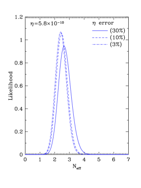
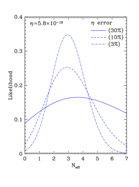
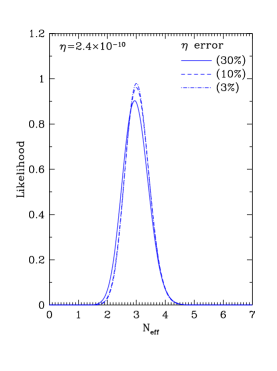
Figure 4: (a) The distribution in $N_{\rm\nu,eff}$ assuming a CMB $\eta$ measurement of Figure 2, and primordial ⁴He & ⁷Li abundances as in eqs. (6) & (7). The curves show the effect of the expected increased accuracy in the CMB determination of $\eta$. (b) Distribution in $N_{\rm\nu,eff}$ assuming a CMB $\eta$ measurement of Figure 2, and a D measurement at the current precision (as in eq. (8)). (c) As in (a), but the a CMB $\eta$ measurement of Figure 3.

With $\eta$ independently and accurately fixed, it becomes possible constrain $N_{\rm\nu,eff}$ with nuclides other than, or in addition to, ⁴He. As seen in Figures 2 and 3, deuterium shows a promising level of sensitivity to $N_{\rm\nu,eff}$. Indeed, D/H has been included in $N_{\rm\nu,eff}$ fitting by several others [9, 11, 12], although ⁴He remained the primary probe of $N_{\rm\nu,eff}$. Figure 4b illustrates the predictive power of a measurement of ${\rm D/H}=(3.0\pm 0.4)\times 10^{-5}$, as found in recent high-redshift determinations (though systematic uncertainties might lead to larger errors). We find that it is possible to obtain a constraint on $N_{\rm\nu,eff}$ to an accuracy $\sigma_{95\%}(\mbox{$N_{\rm\nu,eff}$})=2.2$ with deuterium alone for $\eta_{10}=5.8\times(1\pm 0.03)$. While this constraint is at present weak, it can be sharpened considerably with improved D abundances (see below in §5).

The availability of elements other than ⁴He for neutrino counting has several advantages. Observations of the different elements have very different systematics, so that one can circumvent longstanding concerns about ⁴He observations by simply using other elements. Also, the prospects for improvement in deuterium abundances are better than for ⁴He. For example, many new quasars will be found in the Sloan Survey (see, e.g., [26]), which will lead to a larger set of candidate D/H systems. There is thus reason for optimism that systematics in the determination of primordial deuterium will be sorted out by looking at a large sample.

Turning to the case of lithium, we see from Figures 1 through 3 that the ⁷Li is almost insensitive to $N_{\rm\nu,eff}$. For realistic errors in the observed primordial Li abundance ($\mathrel{\raise 1.29167pt\hbox{$>$\kern-7.5pt\lower 4.30554pt\hbox{$\sim$}}}30\%$ [23]) one cannot expect to use this element as an $N_{\rm\nu,eff}$ discriminant. This may even be a virtue, as the weak dependence of ⁷Li on $N_{\rm\nu,eff}$ means that lithium remains a powerful cross-check of the basic BBN concordance with the CMB, independent of possible variations in $N_{\rm\nu,eff}$.

Of course, the tightest constraints on $N_{\rm\nu,eff}$ would come from combining all available abundances, including ⁴He, in order to exploit its sensitivity to $N_{\rm\nu,eff}$. Even if one chooses to be very conservative regarding the uncertainties in the observed $Y_{p}$, depending on the accuracy of the observed D/H, useful additional constraints can still flow from conservative error bars ($\Delta Y_{p}\sim\pm 0.010$), or from adopting upper or lower bounds to $Y_{p}$.

With $\eta_{\rm CMB}$ in hand, one can use BBN not only to probe the early universe, but also to accurately predict the light element abundances and thus to probe astrophysics. Again, the starting point is the distribution in abundances and $N_{\rm\nu,eff}$ given by eq. (3) and in Figures 2 and 3. One must first address the $N_{\rm\nu,eff}$ dependence of the predictions. For a conservative prediction of the abundances, one can simply marginalize over all allowed $N_{\rm\nu,eff}$, which implicitly assumes that all values in one’s grid are equally likely. One might also simply adopt the range determined from the invisible width of $Z^{0}$ decay, which presently gives $\mbox{$N_{\rm\nu,eff}$}=3.00\pm 0.06$ [28]; this value is sufficiently accurate that one may simply adopt $\mbox{$N_{\rm\nu,eff}$}=3$ in this case, i.e., formally ${\cal L}_{\rm expt}(\mbox{$N_{\rm\nu,eff}$})=\delta(\mbox{$N_{\rm\nu,eff}$}-3)$.

For the case $\mbox{$N_{\rm\nu,eff}$}=3$ we have computed the distribution of predicted light element abundances. Results appear in Figure 5. One should bear in mind that for each $\eta$, the light element predictions are correlated, so that knowledge of one abundance will narrow the distribution for the others.

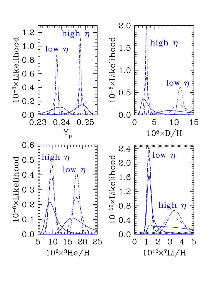
Figure 5: Predicted abundances, illustrated for two possible CMB-determined $\eta$ dubbed high(low) $\eta$ from eq. 4(5). Curves assuming (30, 10, 3%) error in $\eta$ are (solid, dashed, dot-dashed).

With these predictions in hand, one can do astrophysics. For example, deuterium is always destroyed astrophysically [27]. Thus, the ${\rm D/D_{p}}$ ratio in any astrophysical system is the fraction of unprocessed material in that system, and hence constrains the net amount of star formation. In the case of ³He, the stellar nucleosynthesis predictions are uncertain, and the interpretation of dispersion in the present-day observations is unclear; a firm knowledge of the primordial abundance will provide a benchmark against which to infer the Galactic production/destruction of ³He. With regard to ⁷Li, knowlege of the primordial abundance can address issues of stellar depletion and will allow one to better constrain the production of Li by early Galactic cosmic rays [23], and can provide a consistency check on models of halo star atmospheres.

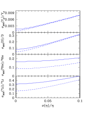
Figure 6: The 95% CL accuracies of the abundance predictions as a function of the CMB accuracy. The adopted $\eta$ is that of eq. (4). Solid line: present BBN theory errors. Dashed line: BBN theory errors reduced by 50%. .

Figure 6 illustrates the impact of improvements in the accuracy of the CMB $\eta$. The solid curves show the fractional error (95% CL) $\sigma_{95\%}(y)/y$ in each element as a function of the CMB precision. We see that for ⁴He, D, and ⁷Li, the precision of the predictions can be improved significantly with improved $\eta$ determinations. This holds until $\sigma_{\eta}/\eta\simeq 0.7\%-3\%$ (Planck’s expected level of precision). At this point, the BBN theory errors begin to dominate; we now turn to this issue.

5 Needed Improvements in Observational and Theoretical Inputs

In anticipation of this new role for BBN, it is important to note the limitations to the power of BBN with $\eta_{\rm CMB}$ given. The sharpness of the predictions is limited by the precision of the observed primordial abundances, and of the nuclear physics inputs. On the observational side, as noted above we can reasonably expect an improvement in D/H as the number of high-redshift absorption line systems increases. To have an idea of the impact of lowering deuterium observational errors, we compute the $N_{\rm\nu,eff}$ prediction using a ${\rm D/H}=3.0\times 10^{-5}$. We show in Figure 7 results with an uncertainty $\sigma({\rm D/H})=0.4\times 10^{-5}$ as before, i.e., $\sigma({\rm D})/{\rm D}=13\%$, as well as $\sigma({\rm D})/{\rm D}=10\%$ and 3%. We see that improved accuracy in the observed D abundances considerably reduces the uncertainty in $N_{\rm\nu,eff}$. Even in the limit of a perfect CMB observation ($\sigma_{\eta}/\eta\rightarrow 0$) the observational and theoretical uncertainty in D leads to a nonzero $N_{\rm\nu,eff}$ width. This reinforces the need to get an accurate determination of D/H as possible.

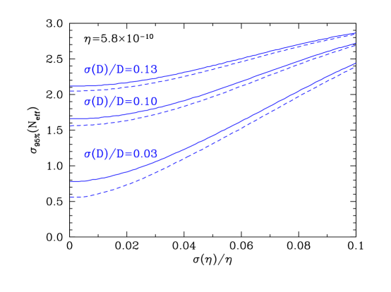
Figure 7: The precision of $N_{\rm\nu,eff}$ determinations for different levels of precision in D and $\eta$ measurements (95% CL).

The other source of uncertainty is the theoretical error which stems from uncertainties in the nuclear inputs. To show the effect of the current nuclear uncertainties, we compute the predicted abundances by arbitrarily reducing the adopted errors [7] by 50%. These appear as the dashed curves in Figures 6 and 7. We see that the theory uncertainties are in fact a minor contributor to the total error budget of $N_{\rm\nu,eff}$, which is dominated by the observational abundance errors. However, for abundance predictions, the theory errors can be important, particularly for ³He and ⁷Li. Of these, the ⁷Li errors are the most important candidate for improvement (e.g., [7]), as an accurate knowledge of primordial ⁷Li can have an immediate impact on studies of Population II stellar evolution, and on early Galactic cosmic rays. On the other hand, our current theoretical and observational understanding of ³He is probably too crude to profit from the high-precision depicted in Fig. 6, though this may change by the time the Planck results are available.

6 Discussion and Conclusions

Upcoming precision measurements of CMB anisotropies will revolutionize almost all aspects of cosmology. These data will allow for an independent and precise measure of the baryon-to-photon ratio $\eta\propto\Omega_{\rm B}h^{2}$, and will thus have a major impact on BBN. As we have shown, even if there is agreement between CMB results and BBN predictions, BBN will not lose its relevance for cosmology, but rather shifts its role and primary focus to become a sharper probe of early universe particle physics and of astrophysics.

At present, the 20% quoted uncertainty in $\eta$ from CMB determinations [1, 3, 4] and the helium abundance of eq. (6) leads to the following 95 % CL upper limits on $N_{\rm\nu,eff}$:

• Using ⁴He and $\eta_{10}=5.8$   $\mbox{$N_{\rm\nu,eff}$}<3.6$

• Using ⁴He and $\eta_{10}=2.4$   $\mbox{$N_{\rm\nu,eff}$}<3.9$

Note that in the first case, we have applied the prior that $\mbox{$N_{\rm\nu,eff}$}\geq 3.0$ [11], while in the second case we have shown the effect of a CMB $\eta$ consistent with the ⁴He and ⁷Li abundances and measured to 20%. The 20% uncertainty in $\eta$, in conjunction with D/H as in eq. (8) (i.e., with a 13% uncertainty) gives a very weak limit on $N_{\rm\nu,eff}$ (i.e., the 95% CL limit is above $\mbox{$N_{\rm\nu,eff}$}=7$). Future CMB determinations will tighten the $N_{\rm\nu,eff}$ bound. While the limit based on ⁴He is relatively unaffected by an improved CMB determination (see Fig. 4), the limit based on D will improve. For example, with a 10% measurement of $\eta$, and with D/H as in eq. (8), the limit is $\mbox{$N_{\rm\nu,eff}$}<5.9$ (95% CL). With a 10% (3%) uncertainty in D/H, the limit to $N_{\rm\nu,eff}$ is reduced to 5.7 (5.4). Finally, the bound will be reduced to $\mbox{$N_{\rm\nu,eff}$}<4.0$, assuming a 3% uncertainty in both $\eta$ and D/H.

With $\eta_{\rm CMB}$ and light element abundances as inputs, BBN will be able to better constrain the physical conditions in the early universe. We have illustrated this in terms of the effective number $N_{\nu,{\rm eff}}$ of light neutrino species. All light element abundances will become available to constrain $N_{\rm\nu,eff}$, allowing for tighter limits and cross checks that are unavailable today. We note in particularly the deuterium measurements alone will be able to obtain useful limits on $N_{\rm\nu,eff}$, independent of the use of ⁴He observations. Also, while we have framed the early universe physics in terms of $N_{\rm\nu,eff}$, one may also bring the power of the CMB inputs to constrain a wide range of physics beyond the standard model [29], and more complicated early universe scenarios such as inhomogeneous BBN [30].

One can also use BBN theory and the CMB $\eta$ to infer primordial abundances quite accurately. This will sharpen our knowledge of astrophysics, with galactic-scale stellar processing probed via deuterium abundances, and stellar nucleosynthesis constrained with ³He and ⁴He, and cosmic rays and stellar depletion tested with ⁷Li.

In anticipation of the CMB results, continued improvements in light element observations and in BBN theory are needed. Reduced (but realistic!) error budgets are the key obstacle in maximizing leverage of the CMB $\eta$. For light element observations, the key issue is that of systematic errors. For BBN theory, nuclear uncertainties now dominate the error budget. Efforts to improve both theory and observations will be rewarded by the ability to do precision cosmology with BBN.

Acknowledgments
The work of K.A.O. was partially supported by DOE grant DE–FG02–94ER–40823.

References

- [1] P. de Bernardis et al., Nature 404, 955 (2000) [astro-ph/0004404]; A. Balbi et al., Astrophys. J. 545, L1 (2000) [astro-ph/0005124]; A. Jaffe, et al. Phys. Rev. Lett. 86, 3475 (2000) [astro-ph/0007333].
- [2] S. Padin, S., et al. Astrophys. J. 549, L1 (2001).
- [3] C. Pryke et al. , (2001) [astro-ph/0104490].
- [4] C.B. Netterfield et al. , (2001) [astro-ph/0104460].
- [5] D. N. Schramm and M. S. Turner, Rev. Mod. Phys. 70, 303 (1998) [astro-ph/9706069]; S. Burles, K. M. Nollett and M. S. Turner, Phys. Rev. D 63, 063512 (2001) [astro-ph/0008495].
- [6] J.M. O’Meara, et al. , (2000) [astro-ph/0011179].
- [7] R.H. Cyburt, B.D. Fields, and K.A. Olive, New Astron., in press (2001) [astro-ph/0102179].
- [8] G. Steigman, D.N. Schramm, and J. Gunn, Phys. Lett. B66, 202 (1977).
- [9] K. A. Olive and D. Thomas, Astropart. Phys. 7, 27 (1997) [hep-ph/9610319]; K. A. Olive and D. Thomas, Astropart. Phys. 11, 403 (1999) [hep-ph/9811444]; E. Lisi, S. Sarkar and F. L. Villante, Phys. Rev. D 59, 123520 (1999) [hep-ph/9901404].
- [10] T. P. Walker, G. Steigman, D. N. Schramm, K. A. Olive and H. Kang, Astrophys. J. 376, 51 (1991); K. A. Olive, G. Steigman and T. P. Walker, Phys. Rept. 333, 389 (2000) [astro-ph/9905320].
- [11] K. A. Olive and G. Steigman, Phys. Lett. B 354, 357 (1995) [hep-ph/9502400].
- [12] C. Y. Cardall and G. M. Fuller, Astrophys. J. 472, 435 (1996) [astro-ph/9603071]; P. J. Kernan and S. Sarkar, Phys. Rev. D 54, 3681 (1996) [astro-ph/9603045] N. Hata, G. Steigman, S. Bludman and P. Langacker, Phys. Rev. D 55, 540 (1997) [astro-ph/9603087]; C. J. Copi, D. N. Schramm and M. S. Turner, Phys. Rev. D 55, 3389 (1997) [astro-ph/9606059].
- [13] B. D. Fields and K. A. Olive, Phys. Lett. B 368, 103 (1996) [hep-ph/9508344].
- [14] M. Zaldarriaga, D. N. Spergel and U. Seljak, Astrophys. J. 488, 1 (1997) [astro-ph/9702157]; J. R. Bond, G. Efstathiou and M. Tegmark, Monthly Not. Royal Astr. Soc. 291, L33 (1997) [astro-ph/9702100]; G. Jungman, M. Kamionkowski, A. Kosowsky and D. N. Spergel, Phys. Rev. D 54, 1332 (1996) [astro-ph/9512139].
- [15] R. E. Lopez, (1999) [astro-ph/9909414].
- [16] S. Hannestad, Phys. Rev. Lett. 85, 4203 (2000) [astro-ph/0005018]. S. Hannestad, “New CMBR data and the cosmic neutrino background,” [astro-ph/0105220].
- [17] J. P. Kneller, R. J. Scherrer, G. Steigman and T. P. Walker, astro-ph/0101386.
- [18] K. A. Olive, E. Skillman and G. Steigman, astro-ph/9611166; B. D. Fields and K. A. Olive, Astrophys. J. 506, 177 (1998) astro-ph/9803297.
- [19] Y.I. Izotov, and T.X. Thuan, Astrophys. J. 500, 188 (1998).
- [20] M. Peimbert, A. Peimbert, and M.T. Ruiz, M. T. Astrophys. J. 541, 688 (2000).
- [21] K.A. Olive, and E. Skillman, E. New Ast., in press, (2001) [astro-ph/0007081].
- [22] P. Bonifacio, P. and P. Molaro, P., MNRAS 285, 847 (1997); S.G. Ryan, J. Norris, and T.C. Beers, Astrophys. J. 523, 654 (1999).
- [23] S. G. Ryan, T. C. Beers, K. A. Olive, B. D. Fields and J. E. Norris, Astrophys. J. 530, L57 (2000) [astro-ph/9905211].
- [24] S. D’Odorico, M. Dessauges-Zavadsky, and P. Molaro, Ast. Astro. (2001) [astro-ph/0102162].
- [25] M. Pettini and D.V. Bowen, (2001) astro-ph/0104474.
- [26] D. P. Schneider et al. Astronom. J. 121, 1232 (2001)
- [27] R. Epstein, J. Lattimer and D.N. Schramm, Nature 263, 198 (1976).
- [28] D. E. Groom et al. [Particle Data Group Collaboration], Eur. Phys. J. C 15, 1 (2000).
- [29] S. Sarkar, Rept. Prog. Phys. 59, 1493 (1996) [hep-ph/9602260].
- [30] H. Kurki-Suonio and E. Sihvola, Phys. Rev. D 63, 083508 (2001) [astro-ph/0011544]; K. Jedamzik, G. M. Fuller and G. J. Mathews, Astrophys. J. 423, 50 (1994) [astro-ph/9312065].