Testing the Cosmic Coincidence Problem and the Nature of Dark Energy

Abstract

Dark energy models which alter the relative scaling behavior of dark energy and matter could provide a natural solution to the cosmic coincidence problem - why the densities of dark energy and dark matter are comparable today. A generalized class of dark energy models is introduced which allows non-canonical scaling of the ratio of dark matter and dark energy with the Robertson-Walker scale factor a(t). Upcoming observations, such as a high redshift supernova survey, application of the Alcock-Paczynski test to quasar pairs, and cluster evolution, will strongly constrain the relative scaling of dark matter and dark energy as well as the equation of state of the dark energy. Thus, whether there actually is a coincidence problem, and the extent of cosmic coincidence in the universe’s recent past can be answered observationally in the near future. Determining whether today is a special time in the history of the universe will be a SNAP.

Recent observations of supernovæ p99 , CMB anisotropies cmb and large scale structure lss ; bahcall point to the presence of a flat universe with a dark energy component. The exact nature of the dark energy is not clear, but it must contribute a significant fraction of the closure density today, and have sufficiently negative pressure to cause an acceleration of the Hubble expansion rate at recent times. A cosmological constant of magnitude $\Omega_{\Lambda}\equiv\rho_{\Lambda}/\rho_{\rm crit}\approx 0.7$ provides an excellent fit to the experimental data, and so the flat $\Lambda$CDM cosmology has become the leading cosmological model.

However, $\Lambda$CDM is beset by several serious theoretical difficulties, which may be characterized as fine-tuning problems. Experimental data require that the vacuum energy density today be of order $\sim(10^{-3}{\rm eV})^{4}$, whereas the natural scale for the vacuum energy density, theoretically, is of order $m_{Pl}^{4}$, $m_{W}^{4}$, or at best $\Lambda_{\rm QCD}^{4}$. Thus some unknown physics must fine-tune $\Lambda$ by 40–120 orders of magnitude below its natural value. This problem is called the cosmological constant problem lambdarefs . Another related but distinct difficulty with $\Lambda$CDM is the so-called “why now?” or coincidence problem. Briefly put, if $\Lambda$ is tuned to give $\Omega_{\Lambda}\sim\Omega_{M}$ today, then for essentially all of the previous history of the universe, the cosmological constant was negligible in the dynamics of the Hubble expansion, and for the indefinite future, the universe will undergo a de Sitter-type expansion in which $\Omega_{\Lambda}$ is near unity and all other components are negligible. The present epoch would then be a very special time in the history of the universe, the only period when $\Omega_{M}\sim\Omega_{\Lambda}$.

The cosmological constant and coincidence problems have led numerous authors to consider alternatives to $\Lambda$CDM which preserve its stunning successes (Type Ia SNe, CMB anisotropies, large-scale structure) but avoid the above difficulties. The modification which involves the smallest departure from conventional thinking is to postulate that the acceleration of the universe is due not to a cosmological constant, but instead to an evolving component with sufficiently negative equation of state; typically one uses a scalar field tracker ; quintessence . The expansion of the universe in such models can mimic that of a universe with a cosmological constant. These models typically fail to address the coincidence problem since matter density and vacuum energy density evolve differently, and are only comparable for some period of time, which is chosen to coincide with the current epoch. To see this, note that if matter and dark energy are coupled only gravitationally, then they are conserved separately, so the matter density scales as $\rho_{M}\propto a^{-3}$ while the dark energy density scales as $\rho_{X}\propto a^{-3(1+w_{X})}$, taking the equation of state parameter $w_{X}=p_{X}/\rho_{X}$ to be constant. Thus, the ratio $\rho_{M}/\rho_{X}\propto a^{3w_{X}}$. Fairly negative equations of state are required to explain the supernova data ptw , $w_{X}\sim-1$. Matter rapidly was therefore dominant over dark energy at even moderate redshift, leading to the coincidence problem. This argument holds true even if $w_{X}$ evolves with redshift. As long as $w_{X}$ is sufficiently negative for recent times, dark energy is dynamically important only today. Equivalently, the total equation of state $w_{\rm tot}=w_{X}\Omega_{X}\approx 0$ in the recent past, even if $w_{X}$ evolves with redshift away from $-1$. To circumvent the coincidence problem requires a more radical departure from conventional cosmology, such as assuming that there is some mechanism relating the effective cosmological constant to the matter density at all times. Several proposed theories possess this property. Such theories involve modifications of gravitation, or nonminimal coupling between dark energy and matter sss ; carroll .

Little is known about the relation between vacuum and matter energy densities over the history of the universe. It is not experimentally known whether there is a coincidence problem, since we have no experimental information on the variation of $\Omega_{\Lambda}$ and $\Omega_{M}$ with time for the recent history of the universe. In the simplest $\Lambda$CDM scenario, in which the vacuum energy is indeed due to a cosmological constant, the densities scale as

$$\rho_{X}\propto\rho_{M}a^{3}.$$ (1)

In a theory with no coincidence problem, one expects

$$\rho_{X}\propto\rho_{M}.$$ (2)

Other theoretical scenarios proposed in the literature entail vastly different evolutions of matter and energy density. It seems premature at this stage to do a detailed fit of data to a particular model (e.g. a scalar field with a particular form for the potential). Rather, we suggest the alternative approach of using the experimental data to constrain the nature of dark energy with minimal underlying theoretical assumptions. A useful starting point is to assume a phenomenological form for the ratio of the dark energy and matter densities (valid from some redshift $z_{\rm max}$ till today),

$$\rho_{X}\propto\rho_{M}a^{\xi},\hbox{ i.e. }\Omega_{X}\propto\Omega_{M}a^{\xi},$$ (3)

where the scaling parameter $\xi$ is a new observable. The special cases $\xi=3$ and $\xi=0$ correspond to $\Lambda$CDM and the self-similar solutions sss , respectively. The value of $\xi$ quantifies the severity of the coincidence problem, and can be constrained by several means, three of which we describe below.

We will assume a flat universe, $\Omega_{M}+\Omega_{X}=1$, throughout. This is not essential, but simplifies the expressions (and is an observational fact cmb ). Energy conservation requires

$$\frac{d\rho_{\rm tot}}{da}+\frac{3}{a}(1+w_{X}\Omega_{X})\rho_{\rm tot}=0,$$ (4)

where $\rho_{\rm tot}=\rho_{M}+\rho_{X}$ is the total density, which gives

$$\frac{\rho_{\rm tot}}{\rho_{0}}=\exp\left[\int_{a}^{1}{da\over a}3(1+w_{X}\Omega_{X})\right].$$ (5)

Taking $w_{X}$ constant gives

$$\rho_{\rm tot}=\rho_{0}a^{-3}[1-\Omega_{X,0}(1-a^{\xi})]^{-3w_{X}/\xi}$$ (6)

where $\Omega_{X,0}$ is the value of $\Omega_{X}$ today. For $\xi=0$, the solution is $\rho_{\rm tot}=\rho_{0}a^{-\beta}$, with $\beta=3(1+w_{X}\Omega_{X})$.

This family of solutions, with three parameters ($\Omega_{X,0},w_{X},\xi$), allows us to parameterize a wide range of possible cosmologies in a simple fashion. $\Omega_{X,0}$ specifies the current density in dark energy, $w_{X}$ specifies its equation of state, and $\xi$ specifies how strongly $\Omega_{X}/\Omega_{M}$ varies with redshift. With this parameterization in hand, we can explore how well future observations can constrain the time evolution of dark energy density, and thereby limit models of dark energy. As we shall show, many of the classical tests proposed to determine the existence and magnitude of the cosmological constant also are well-suited for testing the coincidence problem in dark energy models. Limiting ($\Omega_{X,0},w,\xi$) is a more efficient procedure than trying to individually constrain the multitudinous theoretical models proposed in the literature. In addition, the parameters have a simple interpretation, and two important special cases, $\Lambda$CDM and self-similar models, are included as $\xi=3$ and $\xi=0$ models, respectively.

The first constraint we consider is the redshift-luminosity relation of high-redshift Type Ia supernovæ. The luminosity distance $d_{L}(z)$ to supernovæ is given by

$$d_{L}(z) = c(1+z)\int_{(1+z)^{-1}}^{1}\frac{da}{a^{2}H}$$

$$= \frac{c}{H_{0}}(1+z)\int_{0}^{z}dz(\rho_{\rm tot}/\rho_{0})^{1/2}$$

where $\rho_{\rm tot}$ is given by Eq. (5). The redshift-magnitude relation for the 42 moderate redshift SNe presented in Ref. p99 is unable to distinguish between standard $\Lambda$CDM and a self-similar model with constant $\Omega_{\Lambda}$, as shown in Fig. 1(a). Future observations snap will result in more stringent constraints, as discussed below.

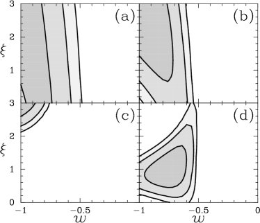
Figure 1: Parameter extraction with future supernova surveys. Panel (a) shows likelihood contours in the ($w,\xi$) plane for the currently known 42 high redshift SNe p99 . Panel (b) illustrates the capabilities of a ground based supernova survey which observes 350 SNe up to redshift $z=1.2$, taking an input $\Lambda$CDM cosmology. Panel (c) shows likelihood contours for 6000 SNe between redshifts $0.3\leq z<1.7$, corresponding to 3 years of SNAP data, again using an input $\Lambda$CDM cosmology. Panel (d) shows the same calculation as (c), but instead using an input cosmology of $\Omega_{X,0}=0.7$, $w=-0.75$, $\xi=1$. Contours correspond to confidence levels of 68%, 95%, and 99%. In all cases we marginalize the likelihood over $\Omega_{X,0}$ using a Gaussian prior centered on $\Omega_{X,0}=0.7$ with width of 0.1.

To determine how well high redshift SNe may be used to distinguish a given set of parameters ${\vec{p}}$ from the true parameters ${\vec{p}}_{0}$, we construct $\chi^{2}$

$$\chi^{2}({\vec{p}},{\vec{p}}_{0}) = \frac{N}{\sigma^{2}}\bigg{(}\int_{0}^{z_{m}}[f({\vec{p}},{\vec{p}}_{0},z)]^{2}W(z)\frac{dz}{z_{m}}$$

$$-\left[\int_{0}^{z_{m}}f({\vec{p}},{\vec{p}}_{0},z)W(z)\frac{dz}{z_{m}}\right]^{2}\bigg{)},$$

$$f({\vec{p}},{\vec{p}}_{0},z)=5\log_{10}\left[\frac{d_{L}({\vec{p}},z)}{d_{L}({\vec{p}}_{0},z)}\right].$$ (9)

Here, $N$ is the total number of SNe, $\sigma\approx 0.2$ is the error in the observed supernova magnitudes, $z_{m}$ is the maximum redshift out to which SNe are followed, and $W(z)$ is a weighting function that describes the redshift distribution of the detected SNe. Note that the second term in Eq. (Testing the Cosmic Coincidence Problem and the Nature of Dark Energy) arises because the supernova absolute magnitude is a free parameter in the fit p99 . For simplicity, we take the redshift distribution to be uniform, $W(z)=1$.

Fig. 1(b–d) displays parameter likelihoods computed using Eq. (Testing the Cosmic Coincidence Problem and the Nature of Dark Energy). We first consider a ground-based survey, capable of detecting 350 SNe up to redshift $z=1.2$. Such a survey would improve the current limits on parameters $w$ and $\xi$ only marginally, disfavoring self-similar models relative to the input $\Lambda$CDM model at the $\sim 1\sigma$ level, as shown in panel (b). We note that this estimate is probably optimistic, since the errors in the SNe magnitudes are likely to be larger than what we have assumed at the high redshift end, where the greatest leverage on $\xi$ is possible. The SNAP satellite, on the other hand, offers the definitive answer to the question of whether there is a coincidence problem. SNAP should observe roughly 6000 SNe up to redshifts $z<1.7$ over its 3-year lifetime, which would allow an unequivocal determination of the presence or absence of a coincidence problem, as shown in panels (c) and (d). We note that most of SNAP’s ability to measure $\xi$ derives from the highest redshift SNe, so there is incentive to follow these events to even higher redshifts ($z\sim 2$) than is currently planned.

SNAP is scheduled to launch late this decade, however other methods may be employed in the interim. Besides high redshift SNe, another means of testing the coincidence problem is the Alcock-Paczyński (AP) test ap ; hui ; jordi . This test distinguishes cosmologies by measuring the product of $H(z)d_{A}(z)$, where $H(z)={\dot{a}}/a$ is the Hubble parameter, and $d_{A}=d_{L}/(1+z)^{2}$ is the angular diameter distance. Following Ref. hui ; jordi , we consider an implementation of this method using the Lyman $\alpha$ forest. If redshift distortions due to peculiar velocities are negligible, then we can analytically estimate the ability of this test to distinguish between cosmologies hui . We place 25 quasar pairs randomly in redshift, with a Gaussian distribution centered on $z=2$, assume separations of $1^{\prime}$, and evaluate the ability of the Alcock-Paczyński test to distinguish various models from the input $\Lambda$CDM model. We plot in Fig. 2 the likelihood contours in $(w,\xi)$ space, again marginalized over $\Omega_{\Lambda,0}$ using a Gaussian prior centered on $\Omega_{\Lambda,0}=0.7$ with width 0.1. Although the Alcock-Paczyński test can rule out a significant class of models, a large region of parameter space is nearly degenerate with 25 quasar pairs. However, the combination of the AP test with other constraints can dramatically shrink the allowed region. In panel (b) of Fig. 2 we plot the joint likelihood obtained by combining constraints from the currently known 42 high redshift SNe p99 with the 25 quasar pairs plotted in panel (a). Although the current SNe data do not constrain $\xi$, when they are combined with the AP constraints, strong limits can be placed on the evolution of $\Omega_{X}/\Omega_{M}$. Since the Alcock-Paczyński test can already be performed today, and the Sloan Digital Sky Survey will provide large numbers of quasar pairs in the imminent future (e.g. sdss ), this method is a promising technique to probe the cosmic coincidence question.

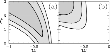
Figure 2: Parameter extraction with the Alcock-Paczyński test. Panel (a) shows likelihood contours (68%, 95%, and 99% respectively) derived by placing 25 quasar pairs randomly in redshift with a Gaussian distribution centered on $z=2$ with width $\Delta z=1$. We use Eq. (6) of Ref. hui to evaluate the ability of the AP test to distinguish various cosmologies from $\Lambda$CDM. In panel (b) we show the joint likelihood (same confidence levels as panel (a)) of the AP test along with the currently known 42 high redshift SNe. The combined constraints severely limit possible models, and lead to excellent determination of $\xi$. In both cases we marginalize over $\Omega_{X,0}$ assuming the same prior as in Fig. 1.

A final example we consider is the evolution of cluster abundances at high redshifts. As is well known, cluster abundances place strong constraints on cosmology; for example, a single $M\approx 10^{15}M_{\odot}$ cluster at $z>0.8$ rules out $\Omega_{M}=1$ with high significance bahcall assuming Gaussian initial fluctuations. Similarly, galaxies observed at high-redshift appear to have formed earlier than predicted by leading models peebles . Our models with $\xi<3$ predict even less evolution than $\Lambda$CDM, because the dark energy remains dynamically important further into the past. Therefore, the presence or absence of clusters at high redshifts $(z>1)$ can place strong constraints on the coincidence problem.

We use the Press-Schechter approximation to estimate the rate of cluster evolution with redshift; see Ref. fan for details. To compare with observations, we plot the number density not as a function of the virial mass, but as a function of the mass enclosed within $1.5h^{-1}$ Mpc, by computing the virial overdensity $\Delta$ using the spherical collapse model eke and rescaling the mass using the profile $M(<r)\propto r^{0.64}$ fan . For simplicity, we assume that observed clusters collapse and virialize at the redshift at which they are observed. Examples of cluster evolution are plotted in the first panel of Fig. 3. As with the other tests discussed above, cluster evolution can clearly discriminate between self-similar models and tracker models. However, it appears that there will be degenerate regions of parameter space.

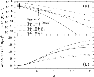
Figure 3: Other methods. In panel (a) we plot the predicted number density of massive clusters for different parameter choices. The self-similar models predict far less evolution between $z\sim 2$ and the present time than $\Lambda$CDM. Data points with errorbars are taken from Ref. fan . In panel (b), we plot comoving volume elements for the same models plotted in the first panel. Note that nearly degenerate models in panel (a) are well separated in panel (b).

Besides the examples described in this work, other probes of the coincidence problem will be possible. At moderate redshifts, number counts of galaxies newman (see Fig. 3) or gravitational lensing statistics kochanek should strongly constrain the evolution of dark energy, if systematic effects such as evolution can be accurately modeled. At higher redshifts, constraints on $\Omega_{X}$ may be derived from Big Bang nucleosynthesis at $z\approx 10^{6}$ or CMB anisotropies at $z\approx 10^{3}$ bean . Given that the dark energy is still so poorly understood, it is not clear whether these high redshift limits may be extrapolated to recent epochs, when the coincidence problem arises. One possible constraint from CMB anisotropies on the recent evolution of dark energy is the normalization of the power spectrum. Normalization using $\sigma_{8}$ and COBE are consistent for standard, low density models, however our models with $\xi<3$ and $w\sim-1$ could ruin this consistency by changing the angular power spectrum on large scales ($l\sim 10$) due to the integrated Sachs-Wolfe effect.

We have shown that several independent methods may be used to test the coincidence problem, as well as test whether the simplest dark energy scenarios are feasible or whether radical departures from conventional thinking are required. All of these measurements are either currently feasible (and in progress), or will soon be forthcoming. Of the methods we discuss, the most definitive conclusions will be possible using the SNAP satellite, which hopefully will fly later this decade. SNAP’s ability to constrain the evolution of $\Omega_{X}$ will be enhanced by following SNe at very high redshift, $z\gtrsim 2$. In the near term, strong constraints may be placed on dark energy using cluster evolution or the Alcock-Paczyński test. We note that if these latter methods give preliminary hints of a departure from standard ($\xi+3w=0$) cosmologies, then it will be imperative to build experiments like SNAP to further study dark energy.

We thank Eric Gawiser, Nao Suzuki, Wallace Tucker and Art Wolfe for helpful discussions. This work was supported in part by the U.S. Dept. of Energy, under grant DOE-FG03-97ER40546. KA was partially supported by NASA under GSRP, and ND acknowledges support from the ARCS Foundation.

References

- (1) S. Perlmutter et al. (The Supernova Cosmology Project), Astrophys. J. 517, 565 (1999); A. G. Riess et al. (High- Supernova Search), Astrophys. J. 116, 1009 (1998).
- (2) P. de Bernardis et al., Nature 404, 955 (2000); A. E. Lange et al., Phys. Rev. D 63, 042001 (2001); C. B. Netterfield et al., astro-ph/0104460; C. Pryke et al., astro-ph/0104490; R. Stompor et al., astro-ph/0105062.
- (3) J. Peacock and S. Dodds, Mon. Not. R. Astron. Soc. 267, 1020 (1994).
- (4) N.A. Bahcall, Phys. Rep. 333–334, 233 (2000).
- (5) S. Weinberg, Rev. Mod. Phys. 61, 1 (1989); S. Carroll, astro-ph/0004075.
- (6) P. J. E. Peebles and B. Ratra, Astrophys. J. Lett. 325, L17 (1988); J. A. Frieman and I. Waga, Phys. Rev. D. 57, 4642 (1998); I. Zlatev, L. Wang and P. J. Steinhardt, Phys. Rev. Lett. 82, 896 (1999).
- (7) R. R. Caldwell, R. Davé and P. J. Steinhardt, Phys. Rev. Lett. 80, 1582 (1998).
- (8) S. Perlmutter, M. S. Turner, and M. White, Phys. Rev. Lett. 83, 673 (1999).
- (9) C. Wetterich, Astron. Astrophys. 301, 328 (1995); P. G. Ferreira and M. Joyce, Phys. Rev. D. 58, 023503 (1998); R. Bean and J. Magueijo, astro-ph/0007199; R. Bean, astro-ph/0104464.
- (10) D. Behnke et al., gr-qc/0102039; S. M. Carroll and L. Mersini, hep-th/0105007.
- (11) SNAP proposal, http:snap.lbl.gov.
- (12) C. Alcock and B. Paczyński, Nature 281, 358 (1979).
- (13) L. Hui, A. Stebbins and S. Burles, Astrophys. J. Lett. 511, 5 (1999).
- (14) P. McDonald and J. Miralda-Escudé, Astrophys. J. 518, 24 (1999).
- (15) D. P. Schneider et al., Astron. J. 120, 2183 (2000).
- (16) P. J. E. Peebles, Astrophys. J. Lett. 483, 1 (1997).
- (17) X. Fan, N. Bahcall, and R. Cen, Astrophys. J. Lett. 490, 123 (1997).
- (18) V. R. Eke, S. Cole and C. S. Frenk, Mon. Not. R. Astron. Soc. 282, 263 (1996).
- (19) J. A. Newman and M. Davis, Astrophys. J. Lett. 534, 11 (2000).
- (20) C. S. Kochanek, Astrophys. J. 466, 638 (1996).
- (21) R. Bean, S. Hansen and A. Melchiorri, astro-ph/0104162; M. Doran et al., astro-ph/0012139; M. Doran and M. Lilley, astro-ph/0104486.