Merger histories in WDM structure formation scenarios

Abstract

Observations on galactic scales seem to be in contradiction with recent high resolution $N$-body simulations. This so-called cold dark matter (CDM) crisis has been addressed in several ways, ranging from a change in fundamental physics by introducing self-interacting cold dark matter particles to a tuning of complex astrophysical processes such as global and/or local feedback. All these efforts attempt to soften density profiles and reduce the abundance of satellites in simulated galaxy halos. In this paper, we explore a somewhat different approach which consists of filtering the dark matter power spectrum on small scales, thereby altering the formation history of low mass objects. The physical motivation for damping these fluctuations lies in the possibility that the dark matter particles have a different nature i.e. are warm (WDM) rather than cold. We show that this leads to some interesting new results in terms of the merger history and large-scale distribution of low mass halos, as compared to the standard CDM scenario. However, WDM does not appear to be the ultimate solution, in the sense that it is not able to fully solve the CDM crisis, even though one of the main drawbacks, namely the abundance of satellites, can be remedied. Indeed, the cuspiness of the halo profiles still persists, at all redshifts, and for all halos and sub-halos that we investigated. Despite the persistence of the cuspiness problem of DM halos, WDM seems to be still worth taking seriously, as it alleviates the problems of over-abundant sub-structures in galactic halos and possibly the lack of angular momentum of simulated disk galaxies. WDM also lessens the need to invoke strong feedback to solve these problems, and may provide a natural explanation of the clustering properties and ages of dwarfs.

1 Introduction

CDM models have been very successful in reproducing the large scale structure properties of the universe (e.g. Bahcall et al., 1999). However, they have lately been facing a state of crisis because of apparent discrepancies between high resolution $N$-body simulations and observations on galaxy scales. One can divide these problems into two categories: the cuspiness of typical L_⋆ galaxy halos on the one hand (cf. Moore et al. 1999a), and the dearth of dark matter satellites in these very same halos on the other (Klypin et al. 1999, Moore et al. 1999b). As a matter of fact, high resolution observations of galaxy rotation curves seem to be quite incompatible with steep dark matter cores (de Blok et al. 2001, even though Van den Bosch et al. (2000) have challenged this idea), and the number of observed satellites of the Milky-Way is about an order of magnitude smaller than that measured in cold dark matter $N$-body simulations (Klypin et al. 1999). Furthermore, micro-lensing experiments toward the galactic centre lead to the conclusion that cuspy dark matter profiles might yield too much mass inside the solar radius (Binney, Bissantz & Gerhard 2000).

These problems have triggered a series of papers devoted to changing the properties of the dark matter itself and making it self-interacting (e.g. Spergel and Steinhardt, 2000; Bento et al., 2000). However, it is still unclear that we need such dramatic changes to reconcile theory and observations as, for instance, massive black holes in the centre of galaxies could alleviate/solve the cusp problem (Merritt & Cruz 2001), and re-ionisation of the universe could get rid of a significant fraction of visible low mass satellites (Chiu et al. 2001). Bearing these possibilities in mind, we adopt a rather conservative view which has the advantage of being well motivated on the particle physics side. To be more specific, we note that, in principle, active neutrino oscillations can naturally produce sterile neutrinos with masses of order 1 keV (Dolgov and Hansen, 2000). Also, such warm particles would preserve a CDM-like scenario of large scale structures, which is known to be quite successful (Colombi et al. 1996; Bahcall et al. 1999).

The outline of the paper is as follows. We first start with a brief description of the initial power spectra in Section 2, then move on to the simulations themselves in Section 3. In Section 4 we analyze the output from our numerical simulations mainly focusing on the merger history in the new WDM models. We finally summarize our results and conclude in Section 5.

2 Warm Dark Matter Power Spectra

In agreement with the combined observations of the cosmic microwave background anisotropies on sub-degree scales by BOOMERanG (de Bernardis et al. 2000) and MAXIMA (Balbi et al. 2000), and of high-redshift supernovas (Riess et al. 1998; Schmidt et al. 1998; Perlmutter et al. 1999), we have chosen a flat universe model with a cosmological constant. More specifically, values for the cosmological parameters in all the simulations presented here are: $\Omega_{0}=$ 0.33, $\Omega_{\Lambda}=$ 0.67, $H_{0}=$ 67 ${\rm{\ }km{\ }s^{-1}}$Mpc^-1, $\sigma_{8}=$ 0.88. We note that in the case of a CDM model, these values also account correctly for the large-scale structure properties of the universe, such as the evolution of cluster abundances (Eke et al. 1998) and the distribution of galaxies (Benson et al. 2001).

The only difference in the power spectra of the three simulations presented here comes from the damping of small-scale density fluctuations due to relativistic free-streaming in the WDM models. More specifically, we have chosen the free-streaming scales, R_f, to be 0.2 and 0.1 $h^{-1}{\ }{\rm Mpc}$ for our WDM simulations, corresponding to smoothing scales — defined as the comoving half-wavelength of the mode for which the amplitude of the linear density fluctuation is divided by two — of 0.72 and 0.33 $h^{-1}{\ }{\rm Mpc}$ respectively and therefore to masses of 0.5 keV and 1.0 keV for the respective warmons (cf. Eq. (1) of Bode, Ostriker and Turok (2000)). The values are summarized in Table 1.

Table 1: Parameter of the WDM models.

	$\Lambda$WDM1	$\Lambda$WDM2
$R_{f}$	0.1 $h^{-1}{\ }{\rm Mpc}$	0.2 $h^{-1}{\ }{\rm Mpc}$
$m_{\rm WDM}$	1.0 keV	0.5 keV

Following Bardeen et al. (1986), the WDM power spectra, P_WDM, are then obtained by multiplying the CDM power spectrum, P_CDM, by the filter function T${}^{2}_{\rm WDM}$, where:

$$T_{\rm WDM}(k)=\exp\left(-\frac{kR_{f}}{2}-\frac{(kR_{f})^{2}}{2}\right).$$ (1)

Fig. 1 shows the initial power spectra which are used as an input for generating the initial conditions of our three different dark matter simulations analyzed in Section 4.

Figure 1: Input power spectra.

Note that these choices for the masses of the warmons are compatible with observed properties of the Lyman-$\alpha$ forest in high-redshift quasar spectra and with the fact that a minimal fraction of baryons has to have already collapsed by z $\approx$ 6 if the universe is to be re-ionized at high-redshift. As a matter of fact, this latter constraint leads to a lower limit for the warmon mass $m_{\rm WDM}\approx 1.2$ keV, which can go down to $m_{\rm WDM}\approx 750$ eV in the somewhat extreme case where the ionizing-photon production efficiency is ten times greater at high redshifts (Barkana, Haiman & Ostriker 2001). On the other hand, such a low value for the lower limit of the warmon mass has also been derived from analysis of artificial Lyman-$\alpha$-spectra extracted from numerical hydrodynamics simulations (Narayanan et al. 2000).

We have not explicitly assigned non-zero initial thermal velocities for particles in the simulations, because as shown by Hogan and Dalcanton (2000) from phase space density arguments, even if present, they would be too small to be relevant on dwarf galaxy halo scales for the masses of the warmons under investigation here. We note that this conclusion is also supported by the recent simulations of Avila-Reese et al. (2000) and Bode et al. (2000) who have included such velocities in their WDM $N$-body-simulations.

3 The $N$-body Simulations

All three simulations were carried out using the multiple-mass Adaptive Refinement Tree code (ART; Kravtsov, Klypin & Khokhlov 1997).

The ART code achieves high force resolution by decreasing the size of grid cells in all high-density regions, using an automated refinement algorithm. These refinements are recursive, which means that refined regions can also be refined, each subsequent refinement having cells that are half the size of the cells in the previous level. This creates a hierarchy of refinement meshes of different resolution focusing on regions of high density where high spatial force resolution is needed. The present version of the code uses multiple time steps on different refinement levels, as opposed to the constant time stepping in the original version of the code. The multiple time stepping scheme is described in detail in Kravtsov et al. (1998).

In addition to these features, the latest version of the ART code also allows the usage of multiple-masses. We started by placing $512^{3}$ particles into the simulation volume according to the input power spectra as given by Fig. 1 and then using the Zeldovich approximation. All these particles were then collapsed in packets of eight until only $128^{3}$ particles were left. Therefore, in order to re-simulate a region of interest with higher mass resolution we would just need to ’unpack’ the high-mass particles within that region which automatically adds the correct high frequency waves to the simulation. The analysis of such runs will be deferred to a companion paper. Nonetheless, as we reduced our initial number of $512^{3}$ particles only by a factor 64 to obtain $128^{3}$ particles, we already reach the interesting mass resolution of $m_{p}\sim 7\cdot 10^{8}$$h^{-1}{\ }{\rm M_{\odot}}$ in the ”low-resolution” runs that we discuss in this paper.

The box size was chosen to be $25$$h^{-1}{\ }{\rm Mpc}$ on a side and the distribution of particles was evolved from a redshift $z=35$ to $z=0$ in 1000 integration steps, reaching refinement level 5 in all three runs. Because of the multiple time stepping, this corresponds to 32000 steps on the finest grid. As we started with a regular grid of $512^{3}$ grid cells covering the whole computational volume we reached a force resolution of 3$h^{-1}{\ }{\rm kpc}$. All these parameters are summarized in Table 2.

Table 2: Specifications of the numerical simulations.

Simulation Parameter
box size	25 $h^{-1}{\ }{\rm Mpc}$
initial redshift	$z_{i}=30$
number of particles	$128^{3}$
integration steps	1000
force resolution	3 $h^{-1}{\ }{\rm kpc}$
mass resolution	$6.89\cdot 10^{8}$$h^{-1}{\ }{\rm M_{\odot}}$

We output snapshots of the simulation at the following redshifts $z=5,4,3,2,1,0.8,0.6,0.5,0.4,0.3,0.2,0.1,0.0$. Then, we identify galaxy halos and their substructure content using a standard friends-of-friends group finding algorithm (FOF, Davis et al. 1985) as well as the more sophisticated Bound-Density-Maxima code (BDM, Klypin & Holtzman 1997). The BDM algorithm finds the positions of local density maxima smoothed out on a certain scale of interest and uses these maxima as centres for calculating e.g. density profiles in a pre-selected number of radially placed bins. While doing so, the program decides whether particles are bound or unbound and removes the latter ones from the halo in an iterative way.

The final halo catalogues (either FOF or BDM) constitute the building blocks of the analysis described in the following section.

4 Analysis

4.1 Visualisation

The first thing we present is the distribution of dark matter particles in a sphere of radius 750 $h^{-1}{\ }{\rm kpc}$ centred around the two most massive halos in all three simulations. A grey-scaled view of the density fields is given in Fig. 2, where the density at each particle position was calculated on a $256^{3}$ cell grid.

There are two things to notice in this plot:

• we clearly see a decrease of substructure (fewer sub-halos) when moving from CDM to WDM scenarios,

• only the left halo (from now on called halo #1) shows a well defined central core. For the right halo (named halo #2) is it difficult to locate the centre not only by eye, but also using the BDM method: this halo is in fact undergoing a merger event, and therefore has a quite different mass build-up history than halo #1.

To sum up, we are left with the fortunate situation where we can study the merger history of two well resolved halos (more than $10^{5}$ particles within the region shown in Fig. 2), one being more relaxed than the other in the CDM structure formation scenario as well as in the new WDM models.

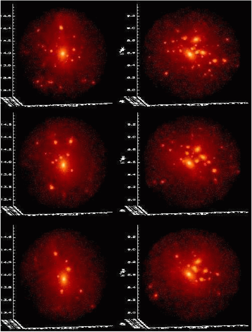
Figure 2: Grey scaled density field of the two most massive galactic halos identified at z=0. The left panel shows halo #1 of mass $9.3\cdot 10^{13}$$h^{-1}{\ }{\rm M_{\odot}}$ (about 135000 particles) and the right panel shows halo #2 weighing $8.2\cdot 10^{13}$$h^{-1}{\ }{\rm M_{\odot}}$ (ca. 120000 particles).

4.2 Power Spectrum Evolution

The first thing to be checked quantitatively is the evolution of the dark matter power spectrum $P(k)$ to see if the filtering scale has left an imprint in today’s power spectrum. Knebe, Islam & Silk (2001) have recently shown that Gaussian features in $P(k)$ are washed out by non-linear effects and it is interesting to see whether or not this also happens with a filtered power spectrum.

Fig. 3 clearly proves that non-linear evolution of the power spectrum boosts the power on small scales so dramatically that we find almost no trace of the ’cut-off’ after a while. Already at a redshift of $z=2$, the WDM spectra has almost converged to the unfiltered CDM spectrum. Therefore, if bias was linear on these scales, we would not expect to find any signature of WDM-like spectra, even in the latest galaxy surveys such as the PSC$z$ (Hamilton & Tegmark 2000).

Figure 3: Power spectrum evolution.

4.3 Mass Function of Halos

The most basic property of a dark matter halo is its mass. In spite of this, mass provides a wealth of information about the formation of structures, especially when computing the (cumulative) distribution of objects $n(>M)$ with mass $M$. As we are expecting the formation of small halos to be damped when filtering the input power spectrum, it indeed seems logical to begin with the study of gravitationally bound objects’ abundances.

Therefore, in Fig. 4 we show halo mass functions in our three dark matter simulations at redshifts $z=0$, $z=1$, $z=2$, and $z=5$. We can clearly see how structures develop in the bottom-up fashion in all three models, although both WDM scenarios exhibit a noticeably different behaviour at the low-mass end. As a matter of fact, we observe in these simulations far less small mass objects than in the CDM simulation, with the deviation being more pronounced and spanning a wider mass range at earlier times. This can be explained by the fact that the formation of low mass objects is somewhat hampered at early times (z $>$ 2 ) by the cut-off in the power spectrum.

On the other hand, we also notice that the mass function in our WDM simulations becomes steeper than in the CDM simulation at the low mass end ($M<3\cdot 10^{10}$$h^{-1}{\ }{\rm M_{\odot}}$) and for smaller redshifts. This phenomenon was also observed by Bode, Ostriker & Turok (2000) and can be explained by formation of “roughly below the free-streaming mass” halos (in our case $1.3\cdot 10^{1}0$$h^{-1}{\ }{\rm M_{\odot}}$ for $\Lambda$WDM1 and $2.7\cdot 10^{1}0$ $h^{-1}{\ }{\rm M_{\odot}}$ for $\Lambda$WDM2), mainly through “pancake” or filament fragmentation. We point out that this is a rather crude estimate as it is clear from Fig. 4, that it affects halos which are several times more massive than these limits. Furthermore, as noted by these authors, as these halos are preferably formed along filaments in a “top-down” scenario, their spatial distributions and epochs of formation contrast with those of a CDM model. This seems to be in better agreement with the clustering measurements of the local population and estimated ages of dwarfs (Peebles 2000; Metcalfe et al. 2000) to which these halos correspond.

Figure 4: Evolution of mass function.

In addition, we plot the number density evolution of objects in the mass range $M\in$[$10^{10}$$h^{-1}{\ }{\rm M_{\odot}}$,$10^{11}$$h^{-1}{\ }{\rm M_{\odot}}$] in Fig. 5. From this figure, one can clearly see that there are fewer small mass halos at high redshifts in WDM simulations. As the difference with the number of CDM halos of the same mass is less important at low redshift, we can therefore conclude that their average formation epoch is much more recent. As previously mentioned, the majority of these objects do not follow the standard CDM “bottom-up” formation process but are rather formed in a “top-down” fashion. We will come back to this statement in the next Section, when investigating the dependence of the position of the objects on the environment.

Figure 5: Evolution of halo abundance for particle groups with mass $M$ in the range [$10^{10}$$h^{-1}{\ }{\rm M_{\odot}}$,$10^{11}$$h^{-1}{\ }{\rm M_{\odot}}$].

Figure 6: Position of halos in the mass range $M\in$[$10^{10}$$h^{-1}{\ }{\rm M_{\odot}}$,$10^{11}$$h^{-1}{\ }{\rm M_{\odot}}$].

Figure 7: Time evolution of the number of halos in the mass range $M\in$[$10^{10}$$h^{-1}{\ }{\rm M_{\odot}}$,$10^{11}$$h^{-1}{\ }{\rm M_{\odot}}$] located within a region of a given density contrast.

4.4 Halo Positions

In the previous Section 4.3 (Fig. 5), we have seen that the evolution of the number density of objects in the mass range $M\in$[$10^{10}$$h^{-1}{\ }{\rm M_{\odot}}$,$10^{11}$$h^{-1}{\ }{\rm M_{\odot}}$] differs significantly from one model to another. At a redshift of $z=5.0$ the abundance of these small mass halos is about a factor of 10 larger in the $\Lambda$CDM simulation than in the $\Lambda$WDM2 simulation, whereas the ratio drops to about 2 at $z=0.0$. We claim that in WDM structure formation scenarios, those objects are primarily formed in high density regions by pancake and filament fragmentation. To back up this statement we first plot in Fig. 6 the projected positions of the halos within the aforementioned mass range onto the $x-y$-plane of the box. We can now see that in the $\Lambda$WDM simulations, low mass halos are indeed tracing the filamentary structure, in contrast to the $\Lambda$CDM simulation where they are much more void-filling. We mention that for clarity, at a given redshift, all plots contain the same number of halos, which means that we have randomly chosen a subset of objects for plotting the positions of halos in the $\Lambda$CDM and $\Lambda$WDM1 models, while using the complete data set for $\Lambda$WDM2. As a complement, in Fig 7, we plot the redshift evolution of the number of low mass halos located in regions of various density contrasts. The density field was computed on a comoving grid composed of $25^{3}$ cells, using a nearest grid point method to assign particles to the grid. This means that each grid cell is exactly 1 $h^{-1}{\ }{\rm Mpc}$ on a side. We then repeat exactly the same procedure, assigning halos with masses between $10^{10}$$h^{-1}{\ }{\rm M_{\odot}}$and $10^{11}$$h^{-1}{\ }{\rm M_{\odot}}$to their nearest grid point. The standard deviations, $\sigma$, for the density field, range from being about 9 times greater than the mean density at $z=0$, when the particle distribution is highly clustered, to 0.7 times lower than the mean density at $z=5$, when the particle distribution is quite smooth. This means that if the density contrast in one region at $z=0$ is greater than 2 $\sigma$, this region is about 18 times denser than the average density of the universe at this redshift. Notice that the standard deviations from the mean density are about the same in the CDM and the WDM simulations, and for all redshifts (within 10 %). It is obvious from this figure that halos in this mass range are more strongly suppressed in low density regions and/or at high redshifts in $\Lambda$WDM cosmologies. On the other hand, in high density regions and at fairly low redshifts, things are quite different: one sees more halos in regions with density contrast between 3 and 4 $\sigma$ (bottom left panel of Figure 7) at $z=0$ in simulation $\Lambda$WDM2 than in simulation $\Lambda$CDM! This is a non ambiguous signature of late “bottom-up” formation of low mass halos in these regions. However, as we are speaking of objects containing only about 20-200 particles we cannot exclude this effect to be due to Poisson fluctuations at the 100% level. But if we check the representation of the initial power spectrum at $z=35$ (cf. Fig. 1) we confirm to sample waves out to at least wavenumber $k\approx 15h{\rm Mpc}^{-1}$ in all three models. This corresponds to a mass scale of roughly $3\cdot 10^{10}$$h^{-1}{\ }{\rm M_{\odot}}$ and hence Poisson noise probably only affects even smaller objects.

Figure 8: Evolution of halo mass for halo #1 and #2 in all three models.

4.5 Merger Histories

As we already mentioned in Section 4.1 we expect the merger histories of the two halos #1 and #2 to be different. Therefore we investigate how the mass of these halos (normalized to the present value) evolves as a function of redshift, and present the results for both halos and all three dark matter models in Fig. 8. Tracing back the merging history of each halo was performed as follows: we first identify all particles belonging to the halo at redshift $z=0$ and locate these particles at redshift $z=0.1$. The halo which now contains the majority of these particles is tagged as the main progenitor and its mass is stored. We repeat the same procedure iteratively out to redshift $z=5.0$. The results are only plotted to redshift $z=1.5$ as the formation time of a halo is normally defined to be the redshift where it weighs half of its present mass. This is about $z=1.0$ for halo #1 and between $z=0.3$ and $z=0.4$ for halo #2.

The figure clearly indicates that two major mergers occurred during the lifetime of halo #2; one around $z=0.5$ and a more recent one between $z=0.2$ and $z=0.1$. These epochs will be particularly interesting when we will analyse the evolution of the density profile of the halo to assess the impact of merger events upon it. Halo #1, on the other hand, builds up its mass mainly via accretion for we do not observe such rapid changes in its merging history.

However, the most important thing to notice in Fig. 8 is that there are almost no differences in the merger histories of CDM and WDM halos. This statement is valid up to $z=5$ and for smaller particle groups not shown in Fig. 8; we followed the merger histories of several objects less resolved than our halos #1 and #2 and did not find any significant discrepancy between CDM and WDM models. This is rather remarkable as there definitely is a smaller number of satellites orbiting those halos at $z=0$ in the WDM scenario, as will be shown in Section 4.6. Furthermore, the final masses of halos #1 and #2 are very close to one another, in all three dark matter simulations, which indicates that these halos have probably been built up from a similar population of small mass objects. In Section 4.6, we actually compute the number of satellites in both halos at various redshifts. It then becomes clear that there are indeed comparable numbers of such small mass halos orbiting in halo #1 and #2 at earlier times. One then has to advocate that in the WDM models, such satellites are disrupted and have their mass redistributed over the whole host halo. Colin, Avila-Reese and Valenzuela (2000) showed that this indeed is the case, as the number of satellites is nearly identical in CDM and WDM at $z=1$ in their simulations: the ”suppression” of small scale structures in massive halos has to result from a disruption of sub-halos rather than from a different merger history.

4.6 Satellite Abundances

One of the problems with CDM models is that high resolution simulations tend to show an order of magnitude more substructure in galaxy size haloes than is actually observed (Klypin et al. 1999, Moore et al. 1999b). One should then require of a viable alternative model that it naturally reduces the abundance of such satellite halos. As the results are generally presented as cumulative velocity distributions for the satellites $N(>v_{\rm circ})$, we have calculated this function for both our halos at redshifts $z=0$ and $z=1$. Results are shown in Fig. 9.

Table 3: Number of satellite galaxies within halo #1 and #2. The mass cuts are measured in $h^{-1}{\ }{\rm M_{\odot}}$.

$z=0.0$
	halo #1		halo #2
	$M>10^{10}$	$M>10^{11}$	$M>10^{10}$	$M>10^{11}$
$\Lambda$CDM	42	26	48	28
$\Lambda$WDM1	32	19	36	24
$\Lambda$WDM2	28	17	28	18
$z=1.0$
	halo #1		halo #2
	$M>10^{10}$	$M>10^{11}$	$M>10^{10}$	$M>10^{11}$
$\Lambda$CDM	29	20	12	8
$\Lambda$WDM1	29	19	12	9
$\Lambda$WDM2	29	19	11	6

Figure 9: Cumulative circular velocity distribution host halo #1 and #2, respectively. Only halos more massive than $10^{10}$$h^{-1}{\ }{\rm M_{\odot}}$ are taken into account.

To generate our data, we have identified all sub-halos using the BDM code and used the maximum of the circular velocity curve to define $v_{\rm max}$. We counted all gravitationally bound particles groups within a sphere of radius $R=1$$h^{-1}{\ }{\rm Mpc}$ around the centre of the halo for $z=0$ and $R=0.5$$h^{-1}{\ }{\rm Mpc}$ for $z=1$, respectively. The total number of satellites found are summarised in Table 3 for two mass cuts $M_{\rm satellite}>10^{10}$$h^{-1}{\ }{\rm M_{\odot}}$ and $M_{\rm satellite}>10^{11}$$h^{-1}{\ }{\rm M_{\odot}}$. Due to the finite number of particles present in our simulated box, we are not able to resolve halos with maximum circular velocities below 50${\rm{\ }km{\ }s^{-1}}$. We are aware that the actual discrepancy between numerical simulation and observations as pointed out by Klypin et al. (1999) and Moore et al. (1999b) appears to be at velocities smaller than this, but we can safely say that our data agrees with the results of Colin, Avila-Reese & Valenzuela (2000) when extrapolating their distribution function to our velocity range. Moreover, at $z=0$, we already observe a drop in the number density of satellites with $v_{\rm max}\approx 50$${\rm{\ }km{\ }s^{-1}}$(cf. Fig. 9), which is all the more pronounced when the mass of the warm dark matter particle $m_{\rm WDM}$ is low.

We have already seen that the masses and mass histories of the two halos are quasi identical irrespective of the model, but we count fewer satellites in the WDM scenarios. How can this happen? One needs to go back to $z=1$ to understand the origin of this puzzle. At this redshift, we see (both in Fig. 9 and Table 3) that the number of sub-halos is indistinguishable between our models; even the distribution functions $N(>v_{\rm circ})$ can be superimposed. We therefore conclude that the same number of satellites are in place by $z=1$ in both the WDM and CDM simulations, but that for the former, they are more easily disrupted during the relaxation process of the host halo. This is also shown in Fig. 7, where we see that in regions of very high density contrast ($>5\sigma$), and at high redshifts, the number of small mass halos is about the same, in all three simulations. This therefore provides a natural explanation as to why merger histories are so similar for massive halos, in WDM and CDM simulations. However, one should bear in mind that the equality of the number of satellites for e.g. halo #1 at $z=0$ and $z=1$ in the $\Lambda$WDM2 simulation does not mean that these sub-halos have survived unaltered. These numbers are the result of a competition between continuous destruction and accretion of satellites during the merging history of each (host) halo. Therefore, numbers in Table 3 actually indicate that the rates at which these two processes (destruction and accretion) occur, become almost identical for halos formed in the $\Lambda$WDM2 structure formation scenario.

Figure 10: Density profiles for halo #1 in all three simulations at redshift $z=0$. The curves in each panel are shifted by factors of ten downwards for clarity and correspond to (from top to bottom): $\Lambda$CDM, $\Lambda$WDM1, and $\Lambda$WDM2.

Figure 11: Density profiles for halo #2 in all three simulations at redshift $z=0$. The curves in each panel are shifted by factors of ten downwards for clarity and correspond to (from top to bottom): $\Lambda$CDM, $\Lambda$WDM1, and $\Lambda$WDM2.

4.7 Density Profiles

We now turn to the radial distribution of mass in the halos by measuring the density profiles of the two most massive halos #1 and #2 for a series of redshifts between $z=1.0$ and $z=0.0$. We fit the data to profiles of the form proposed by Navarro, Frenk & White (1997):

$$\frac{\rho(r)}{\rho_{c}}=\frac{\delta_{c}}{r/r_{s}(1+r/r_{s})^{2}}\ ,$$ (2)

where $\rho_{c}$ is the critical density, $\delta_{c}$ a characteristic (dimensionless) over-density and $r_{s}$ a scale radius. We define the virial radius $r_{\rm vir}$ of the halo to be the radius where $\rho(r_{\rm vir})/\rho_{c}=200$. This radius is then used to calculate the concentration parameter $c_{1/5}$, which is defined as the ratio of the virial radius $r_{\rm vir}$ and a scale radius $r_{1/5}$, where 1/5 of the virial mass is contained:

$$c_{1/5}=r_{\rm vir}/r_{1/5}\ .$$ (3)

This definition of the scale radius is more meaningful for the cases where we can not fit the data sufficiently well to the NFW profile as given by Eq. (3). This occurs mainly when the halo has undergone a recent major merger. Results can be seen in Fig. 10 and Fig. 11 which show the density profiles along with our best fit NFW profiles for halo #1 and #2, respectively. The error bars indicated by vertical lines for each bin in the density profile figures (Fig. 10, Fig. 11, and Fig. 13) are simply Poissonian error bars.

These figures should be viewed with Fig. 8 in mind; we know that for halo #1 the first major merger happened between redshift $z=1.5$ and $z=1.0$ and that is reflected by a steeper slope of the density profile in the inner regions than predicted by the best fit NFW model. The same situation can be observed from redshift $z=0.4$ onwards where the profile starts to steepen albeit less markedly, while the mass history indicates heavy accretion activity (or minor merger events). A corresponding phenomenon is found for halo #2 in Fig. 11. For this latter, the two significant mergers occur between redshifts $z=0.5$ and $z=0.4$ and $z=0.2$ and $z=0.1$, causing a steepening of the inner density profile in all three (CDM as well as WDMs0 simulations. We also tried to fit our data to the even steeper profile proposed by Moore et al. (1999a) having an asymptotic slope $\rho(r)\propto r^{-1.5}$, but we were not able to obtain sensible $\chi^{2}$ values.

However, in Fig. 12 we plot the concentration parameter $c_{\rm 1/5}$ against redshift and do not find any abrupt changes or jumps for the merger events identified in Fig. 8. The only noticeable trend is a nearly constant concentration parameter $c_{\rm 1/5}$ for halo #2. We stress that the fits of the density profiles were only performed up to the virial radius of the halos (i.e. the radius where $\rho(r)$ drops below 200 $\rho_{\rm crit}$). For halo #2 we notice a moderate overshoot in the density profile at large distances from the centre, and at nearly all redshifts. This is due to the fact that the progenitors of this halo all have important masses and the centre of the profile is located at the centre of the most massive one, therefore the most distant progenitor will create an over-density which is not smeared out by the spherical averaging process.

Finally, we point out that there are no obvious different trends in the three different models: density profiles for halos in CDM and both WDM models all show the same behavior, with concentrations being only marginally smaller for WDM halos than for corresponding CDM ones.

Figure 12: Redshift evolution of the concentration parameter $c_{\rm 1/5}$ for the two most massive halos #1 and #2.

As already mentioned by other groups (Colin, Avila-Reese & Valenzuela 2000 and Bode, Ostriker & Turok 2000) one should expect the effect of a loss of concentration to be more pronounced for satellite sub-halos orbiting in the host halos #1 and #2. To verify this, we identified the four most massive satellites ($M_{\rm satellite}\approx(1-10)\cdot 10^{12}$$h^{-1}{\ }{\rm M_{\odot}}$which roughly agrees with 1000 – 10000 particles per satellite) in both halos at redshifts $z=0.0$ and $z=1.0$ and fitted their density profiles again with the NFW profile given by Eq. (3). Even though the data is more noisy for these halos, it is rather well described by such a profile, as can be seen from Fig. 13. We notice that the Poissonian error bars are systematically larger for halo #2 satellites in our $\Lambda$WDM2 simulation, due to a greater sensitivity to the tidal perturbations induced by the very recent merger. These satellites are also slightly less massive than in the other simulations. It should be noted that, as these satellites are embedded in the host halo, one cannot, in all cases, define their virial radius via $\rho(r_{\rm vir})/\rho_{c}=200$. Their profiles sometimes flatten (or rise) and we therefore manually truncated the halos in these cases. We then fitted their density profiles up to either the virial radius or the point where the profile flattened. We also computed the mean concentration $c_{\rm 1/5}$ (averaged over the four satellites). Values for these quantities are shown in Table 4. This time, one can see a trend for WDM sub-halos to have smaller concentrations than their CDM counterparts. This holds at least for the more relaxed structure of halo #1 whereas the overall concentrations for the satellites orbiting in halo #2 are generally smaller because they are still in the process of merging, and the differences between the three dark matter models are therefore less pronounced. An estimate of the robustness of these results can be obtained by comparing the NFW fits to the measured profiles in Fig. 13 where we only show the fits to the satellites found in halo #1 and halo #2 at redshift $z=0.0$. The concentration parameters are indeed well determined.

Figure 13: Density profiles for the four most massive satellites within halo #1 (left panel) and halo #2 (right panel) at $z=0.0$. For legibility, the profiles in each plot are shifted downwards by factors of 10 and correspond to (from top to bottom): $\Lambda$CDM, $\Lambda$WDM1, and $\Lambda$WDM2.

Table 4: Average concentration parameters $c_{\rm 1/5}$ for satellites.

	halo#1		halo#2
	$z=0.0$	$z=1.0$	$z=0.0$	$z=1.0$
$\Lambda$CDM	7.065	3.783	4.360	3.603
$\Lambda$WDM1	5.967	3.004	3.992	3.517
$\Lambda$WDM2	4.475	3.376	4.145	3.296

4.8 Shapes of Halos

The last section strongly argued in favour of a universal density profile common to CDM and WDM halos; even satellite halos were found to be well fitted by NFW profiles. However, there is still room for subtle differences in the shapes of the halos as the computation of density profiles implies redistributing particles inside spheres.

Figure 14: Axis ratios ($a>b>c$) for halos more massive than $3.5\cdot 10^{12}$$h^{-1}{\ }{\rm M_{\odot}}$ (5000 particles).

Therefore, we have measured the triaxiality of all halos containing more than 5000 particles ($M>3.5\cdot 10^{12}$$h^{-1}{\ }{\rm M_{\odot}}$) using the usual definition:

$$T=\displaystyle\frac{a^{2}-b^{2}}{a^{2}-c^{2}}$$ (4)

where $a>b>c$ are the eigenvalues of the inertia tensor. Values for a b and c can be read off of Fig. 14, whereas Table 5 gives the value of T for the two most massive halos #1 and #2.

From Fig. 14 it is difficult again to pin down any obvious difference between CDM and WDM simulated halos. Only Table 5 might indicate that the two most massive WDM halos are marginally more spherical than their CDM counterparts (a value of $T=1.0$ represents a prolate halo whereas $T=0.0$ means that the halo is oblate).

Table 5: Triaxiality parameter $T$ for the two most massive halos #1 and #2.

halo	$\Lambda$CDM	$\Lambda$WDM1	$\Lambda$WDM2
#1:	0.97	0.94	0.88
#2:	0.90	0.70	0.70

4.9 Angular Momentum

Another crucial issue in cosmological simulations of galaxies is the angular momentum of simulated disks. There can only be two reasons why it is too low: either the halos in which the disks sit do not supply enough angular momentum to the baryons in the first place, or these baryons transfer too much of this angular momentum back to the dark matter when they cool to form the disk. Sommer-Larsen and Dolgov found that the specific angular momentum of their disks was higher in WDM simulations than in CDM ones. Admitting that their result holds, we can try to answer the question as whether it is for one reason or the other, even though we do not have a cosmological hydrodynamic simulation. For each individual halo containing more than 100 particles ($M>7\cdot 10^{10}$$h^{-1}{\ }{\rm M_{\odot}}$) we therefore computed the angular momentum according to

$$\vec{J}=\sum_{i=1}^{N}m_{i}\vec{r}_{i}\times\vec{v}_{i}\ .$$ (5)

This value is used to construct the dimensionless spin parameter:

$$\lambda=J\sqrt{|E|}/(GM^{5/2})\ .$$ (6)

Figure 15: Spin parameter distribution in all three models for redshifts $z=0.0$, $z=0.2$, $z=0.5$, and $z=1.0$. Lines show fits obtained using the log-normal distribution given by Eq. (7).

It has been pointed out before by several authors that the distribution of this parameter follows a log-normal distribution showing little evolution with redshift as well as little sensitivity to the cosmological model (e.g. Frenk et al. 1988; Warren et al. 1992; Cole & Lacey 1996; Gardner 2000, Maller, Dekel & Somerville 2001):

$$n(\lambda)=\displaystyle\frac{1}{\lambda\sqrt{2\pi}\ \sigma_{0}}\exp\left({-\frac{\ln^{2}(\lambda/\lambda_{0})}{2\sigma_{0}^{2}}}\right)$$ (7)

Table 6: Redshift evolution of $\lambda_{0}$ when fitting spin parameter distribution to Eq. (7).

	$z=0.0$		$z=0.2$		$z=0.5$		$z=1.0$
	$\lambda_{0}$	$\sigma_{0}$	$\lambda_{0}$	$\sigma_{0}$	$\lambda_{0}$	$\sigma_{0}$	$\lambda_{0}$	$\sigma_{0}$
$\Lambda$CDM	0.040	0.693	0.054	0.681	0.069	0.658	0.093	0.682
$\Lambda$WDM1	0.036	0.707	0.046	0.717	0.061	0.690	0.086	0.703
$\Lambda$WDM2	0.034	0.716	0.042	0.723	0.052	0.742	0.082	0.768

The first step is to check if this also holds for WDM simulations. In Fig. 15 we show the fits of our numerical data using Eq. (7) at $z=0.0$, $z=0.2$, $z=0.5$, and $z=1.0$. This figure is supplemented with the best fit values for the parameters $\lambda_{0}$ and $\sigma_{0}$ in Table 6. These results show that there is no clear correlation of the spin parameter with the dark matter particle mass, although one might argue for a marginal tendency of the halos to have slightly lower spin parameters in the WDM models.

One can also wonder what effect a recent merger event has on the spin parameter. To answer this question we followed both spin histories of massive halos #1 and #2, and plotted the results in Fig. 16. There is no accidental evolution for halo #1 which mainly built up its mass via a steady accretion flow of material (cf. Fig. 8). But the situation looks different for halo #2. For this latter, one can clearly spot the major merger happening between $z=0.5$ and $z=0.4$ and possibly guess that another significant merger has happened around $z=0.1$. But again, there is little (if any) difference between $\Lambda$CDM and the two $\Lambda$WDM models. Changes in angular momentum occurred in a similar fashion in all three models.

Figure 16: Spin parameter evolution for the two halos #1 and #2.

Inspired by the recent results from Bullock et al. (2000) regarding a universal angular momentum profile we also calculated the mass distribution of angular momentum for the two halos #1 and #2. This was done by computing the angular momenta $\vec{J}$ of logarithmically spaced shells (i.e. the same ones that were used for the density profile). The specific angular momenta were obtained by simply dividing the mass enclosed within each shell so that $j(r)=|\vec{J}(r)|/M(r)$. Finally, the shells were sorted in order of increasing $j$ and we looped over all possible $j$s from $j_{\rm min}$ to $j_{\rm max}$, counting the cumulative mass in shells with specific angular momentum less than $j$. The results can be seen in Fig. 17 where we also present the redshift evolution of this mass distribution of angular momentum for both halos.

Figure 17: Mass distribution of specific angular momentum for the two halos #1 and #2 at various redshifts.

The first thing we need to mention is that we were not able to fit the profile suggested by Bullock et al. (2000) to our data. Instead we find that the data is better described by the following formula:

$$M(<j)=\mu j^{\alpha}/(j_{0}+j)^{\alpha}$$ (8)

with $\alpha\approx 2$. Those fits are presented as curves in Fig. 17 whereas the data is given by the histograms. But we need to stress that our $M(<j)$ derivation slightly differs from Bullock et al. as we used spherical shells in contrast to their construction of mass elements. Moreover, the power index $\alpha$ mainly affects the ”central” parts of the distribution where $j$ is less than about 6-7% of $j_{\rm max}$.

However, it is clear from this figure that these distributions are fairly similar, especially at redshift $z=0$, and that there is no trend of a different time evolution between WDM and CDM halos.

As previously mentioned, Sommer-Larsen and Dolgov (2000) found that galactic disks had higher specific angular momenta in their tree-SPH WDM simulations than in their CDM simulations. When one considers the results presented above, it seems fairly safe to claim that this is entirely due to a different transfer of angular momentum between gas particles and dark matter sub-structures in their simulations: the only noticeable difference in dark matter properties between WDM and CDM being the suppression of these sub-structure in relaxed WDM halos.

5 Conclusions

We have run and analysed two $\Lambda$WDM $N$-body simulations with realistic warmon masses (0.5 and 1.0 keV) and compared them to an identical $\Lambda$CDM simulation. By identical, we mean that the initial conditions in all the simulations were the same, except for the cut-off of the power spectrum of the density field on small scales, characteristic of warm dark matter particles typical free-streaming scales. More specifically, we have focussed on the detailed analysis of two (cluster-sized) halos with mass $M\approx 9\cdot 10^{13}$$h^{-1}{\ }{\rm M_{\odot}}$, one of which was found to be well relaxed, and the other still in the process of virializing. In all the simulations, we have studied the properties of these quite massive halos, but also of the substructure they contained (mainly galaxy-sized objects). We found that:

• there are fewer sub-halos in WDM host halos when the mass of the dark particle drops. This is due to the fact that in WDM scenarii satellites are more fluffy than in CDM scenarii (their concentration parameter is lower), which makes them more prone to disruption during the relaxation processes of the host halo.

• the formation times of small mass halos ($M\sim 10^{10-11}$$h^{-1}{\ }{\rm M_{\odot}}$) and their mode and sites of formation are different: a vast fraction of WDM small halos form in a top-down fashion by fragmentation of filaments at low redshifts, whereas in CDM simulations they all form in a bottom-up way through the merging of even smaller objects at high redshifts.

• the average ages of dwarfs is sensibly higher in CDM models, and these small galaxies are more void-filling than their WDM counterparts which track more closely the cosmic web.

• the merger and spin parameter histories are almost identical for CDM and WDM halos above this mass.

• density profiles of all our halos and sub-halos are well fit by NFW profiles.

• specific angular momentum profiles can be fitted by a universal profile as suggested by Bullock et al. (2001) even though we found a steeper drop at the low $j$ end of that distribution. However, all curves are fairly similar in all models, to such an extent that the resolution of the angular momentum problem of disk galaxies in WDM simulations (which was claimed by Sommer-Larsen & Dolgov 2000) has to be entirely due to a different transfer between gas and dark matter substructures.

Comparing our work to previous analysis of a similar type, we find good agreement with the results of Colin et al. (2001), and we believe that the discrepancy between our work and that of Bode, Ostriker and Turok (2000) concerning concentration parameters can be explained by differences either in the warmon masses (they used lighter particles in several of their simulations) or in the data analysis. More specifically, we used $c_{\rm 1/5}$ as a measure of the concentration of our halos which systematically yields lower values than the usual NFW concentration parameter that they use (Avila-Reese et al. 1999; Colin et al. 2000). However, to really settle the issue, and quantify possible differences in the cores of massive WDM halos and in the overall reduction of the total number of small halos certainly requires more simulations and of higher resolution to be performed. As a conclusion, we stress that even though we showed that WDM is not the ideal solution to the so-called CDM crisis, it is still worth exploring seriously, especially if more accurate data confirms that dwarf galaxy properties are in real conflict with CDM model predictions.

References

- [avila99] Avila-Reese V., Firmani C., Klypin A., Kravtsov A.V., MNRAS 310, 527 (1999)
- [avila00] Avila-Reese V., Colin P., Valenzuela O., D’Onghia E., Firmani C., astro-ph/0010525
- [bahcall97] Bahcall N.A., Fan X., Cen R., ApJ Lett. 485, 53 (1997)
- [bahcall99] Bahcall N.A., Ostriker J.P., Perlmutter S., Steinhardt P.J., Science 284, 1481 (1999)
- [bardeen] Bardeen J.M., Bond J.R., Kaiser N., Szalay A.S., ApJ 304, 15 (1986)
- [barkana] Barkana R., Haiman Z., Ostriker J.P., astro-ph/0102304
- [balbi] Balbi A., et al., astro-ph/0005124
- [benson] Benson A., et al., astro-ph/0103092
- [bento] Bento M.C., et al. Phys. Rev. D 62, (2000)
- [binney] Binney J., Bissantz N., Gerhardt O., ApJ Lett. 537, 99 (2000)
- [blok] de Blok W.J.G., McGaugh S.S., Bosma A., Rubin V.C., astro-ph/0103102
- [bode] Bode P., Ostriker J.P., Turok N., astro-ph/0010389
- [bullock] Bullock J., Dekel A., Kolatt T.S., Kravtsov A.V., Klypin A.A., Porciani C., Primack J.R., astro-ph/0011001
- [chiu] Chiu W.A., Gnedin N.Y., Ostriker J.P., astro-ph/0103359
- [cole96] Cole S., Lacey C., MNRAS 281, 716 (1996)
- [colin00] Colin P., Avila-Reese V., Valenzuela O., ApJ 542, 622 (2000)
- [colombi] Colombi S., Dodelson S., Widrow L.M., ApJ 458, 1 (1996)
- [debernardis] de Bernardis P., et al., Nature 404, 955 (2000)
- [couchman91] Couchman H.M.P, ApJ Lett. 368, 23 (1991)
- [davis] Davis M., Efstathiou G., Frenk C.S., White S.D.M., ApJ 292, 371 (1985)
- [dolgov] Dolgov A., Hansen S. H., hep-ph/0009083
- [dressler] Dressler A., Shectman S.A., Astron. J. 95, 985 (1988)
- [eke96] Eke V.R., Cole S., Frenk C.S., MNRAS 282, 263 (1996)
- [eke98] Eke V.R., Cole S., Frenk C.S., Henry J.P., MNRAS 298, 1145 (1998)
- [frenk88] Frenk C.S., White S.D.M., Davis M., Efstathiou G., ApJ 327, 507 (1988)
- [gardner00] Gardner J., astro-ph/0006342
- [hamilton] Hamilton A., Tegmark M., astro-ph/0008392
- [klypin97] Klypin A.A., Holtzman J., astro-ph/9712217
- [klypin99] Klypin A.A., Kravtsov A.V., Valenzuela O., Prada F., ApJ 522, 82 (1999)
- [knebe99] Knebe A., Müller V., A&A 341, 1 (1999)
- [knebe00] Knebe A., Müller V., A&A 354, 761 (2000)
- [maller] Maller A.H., Dekel A., Somerville R.S., astro-ph/0105168
- [meritt] Meritt D., Cruz F., astro-ph/0101194
- [moore99a] Moore B., Quinn T., Governato F., Stadel J., Lake G., MNRAS 310, 1147 (1999)
- [moore99b] Moore B., Ghigna S., Governato F., Lake G., Quinn T., Stadel J., Tozzi P., ApJ Lett. 524, 19 (1999)
- [narayanan] Narayanan V.K., Spergel D.N., Davé R., Ma C.P., astro-ph/0005095
- [perlmutter] Perlmutter S., et al., ApJ 517, 565 (1999)
- [pinkney] Pinkney J., Roettiger K., Burn J.O., Bird C.M., ApJ 104, 1 (1996)
- [press] Press W.H., Schechter P., ApJ 187, 425 (1974)
- [riess] Riess A.G., et al., Astron. J. 116, 1009 (1998)
- [sahni] Sahni V., Colos P., Phys. Rep. 262, 2 (1995)
- [schmidt] Schmidt B. P., et al., ApJ 507, 46 (1998)
- [seljak] Seljak U., Zaldarriaga M., ApJ 469, 437 (1996)
- [spergel] Spergel D.N., Steinhardt P.J., Phys. Rev. Lett. 84, 3760 (2000)
- [warren92] Warren M.S., Quinn P.J., Salmon J.K., Zurek W.H., ApJ 399, 405 (1992)