Spectrophotometric Evolutionary Models
for Tidal Dwarfs

Abstract

We describe our procedure to model Tidal Dwarf Galaxies in the context of our evolutionary synthesis code. Our analysis shows strong contributions of gaseous emission lines to optical colors and of continuum emission to NIR colors during the burst phase. This underlines the importance of including both types of emission when modeling any type of star-bursting galaxies.

1 Introduction

Tidal Dwarf Galaxies (short TDGs) are formed of stars and gas from (outer) parts of spiral galaxies ripped out from the disk(s) during interactions and merging events (see Duc & Mirabel, 1994; Duc et al., 1997, 2000). If they get tightly bound they may remain stable and survive as independent dwarf galaxies, if they do not fall back onto the interacting system.

Due to the current formation scenario (see Weilbacher & Duc, this volume) TDGs can contain both old and young stellar components in various proportions, inherited from the progenitor spiral disk and created in a starburst within the tidal tail, respectively. See Duc & Mirabel (1998) and Duc et al. (2000) for the most extreme cases. A special star formation history is therefore required to appropriately model TDGs.

Spectrophotometric modelling of these objects will help us to understand their further evolution:

• How bright can they get?
  

• How strong are the starbursts?
  

• How much do they fade?
  

2 Model Implementation

Ingredients of our evolutionary synthesis models (see Weilbacher et al., 2000, for details) are Geneva stellar tracks in 3 different metallicities Z1=0.001, Z2=0.004, Z3=0.008$\approx$Z_⊙/2 and the Scalo IMF. To approximate a TDG-specific star formation history we include an underlying old component with constant SFR for the progenitor disk and a young component due to a starburst of varying duration and intensity which can be modeled as instantaneous, exponentially declining or Gaussian-shaped burst (possibly more realistic). Each model then defines a burst strength

$$b=\dfrac{\mathrm{stellar\ mass\ from\ burst}}{\mathrm{total\ stellar\ mass}}$$

To include gaseous emission into our code we use Lyman continuum photons (Schaerer & de Koter, 1997), gas continuum emission, and emission lines appropriate for each metallicity. The emission line ratios for the three metallicities are taken from spectra observed by Izotov et al. (1994, 1997) and Izotov & Thuan (1998) and theoretical modelling (Stasińska, 1984) for low metallicity (Z1, Z2) and medium metallicity (Z3), respectively. The line ratios we extracted from these works are displayed in Fig. 1.

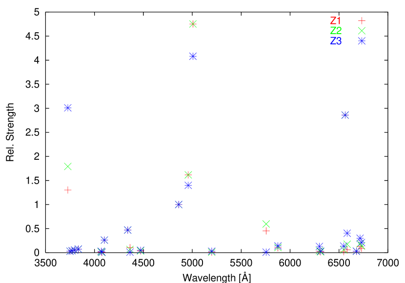
Figure 1: Line ratios normalized to H_β for our three metallicities.

2.1 Broad Band Colors

The contribution of emission lines and gaseous continuum to the broad-band colors varies with burst age, strength, and metallicity and strongly depends on the wavelength of the filter, as shown in Fig. 2 for two different ages within the same burst and two different metallicities.

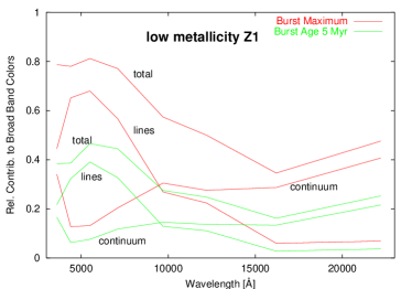
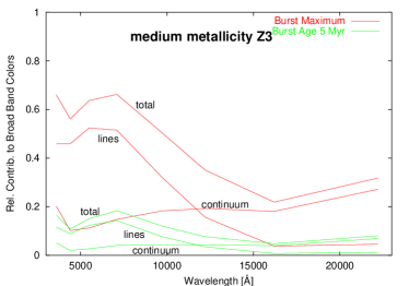
Figure 2: Contribution of the gaseous continuum and line emission for two metallicities and two burst ages, $b=0.18$.

It is obvious that during the beginning of the burst the optical colors are dominated by the gaseous emission and that the stellar contributions only play a minor role, while they gain importance a few Myrs after the maximum of the burst. The contributions of emission lines and continuum to the broad-band filters therefore have to be taken into account.

Using two-color diagrams we can now compare the photometry of observations and models, to derive burst age, burst strength, and further evolution. In the case shown in Fig. 3 the model with Z1 is fitting better than the model with Z3. For a detailed discussion of this type of diagram see Weilbacher et al. (2000). If photometry in more than three filters is available, the results will be more accurate, especially when including NIR colors.

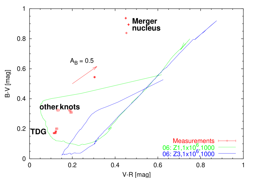
Figure 3: Two-color diagram $B-V$ vs. $V-R$ for two metallicities with example data points.

2.2 Spectra

To better constrain the parameters, obtain information about internal extinction, and disentangle ambiguities from metallicity, burst age, and burst strength, we also want to compare with spectra of the objects. We therefore create model spectra at several timesteps during and after the burst, using the stellar library from Lejeune et al. (1997, 1998). We had to interpolate the spectra linearly to 2 Å resolution in the optical to properly add Gaussian-shaped emission lines with typical FWHM onto the synthetic galaxy spectra.

Three spectra of a strong starburst with different metallicities at the same age are shown in Fig. 4a. The line fluxes vary considerably due to changes in the metallicity of the gas and different temperatures and luminosities of the young stars. Three more spectra show the time evolution during the burst for the model with metallicity Z2 in Fig. 4b. The Balmer line fluxes and the strength and slope of the continuum can be used to select the best fit model for a given observation.

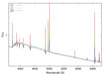
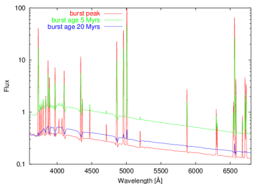
Figure 4: Synthetic spectra for (a) three different metallicities and (b) three different ages.

3 First Results

As an example of the procedure we use data of a typical TDG. We first use the broad-band colors to derive a good estimate of the burst strength and a first guess of the burst age (as in Fig. 3). The observed metal abundance will tell us which metallicity to use for in the models. We then compare the observed equivalent width of H_β with the equivalent width from these models (two models are shown in Fig. 5a). One of the possible ages for each model generally turns out to be consistent with the age estimated from the broad-band photometry.

The dereddened observed spectrum of the same TDG plotted together with the model spectra of weak and strong bursts preselected for the correct burst age from their H_β equivalent widths are given in Fig. 5b. We can finally select the correct model using the slope of the continuum of the different models.

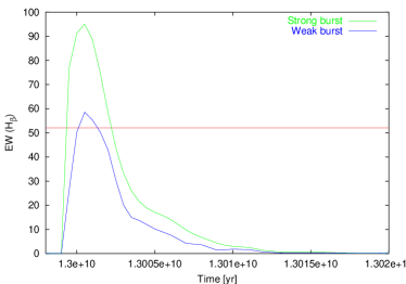
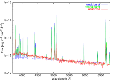
Figure 5: (a) The evolution of EW(H_β). The straight line is the observed value. (b) Models with two different burst strengths at the allowed age compared with the observed spectrum.

The results from the broad-band colors are confirmed in this case by using the spectral information, a strong burst with $\sim$20% young stars and an age of 3 Myrs best explains the observed spectrum.

4 Outlook

The models shown here are only examples of what we plan to do. We will compute a grid of spectral evolutionary models similar to the photometric ones of Weilbacher et al. (2000) with our updated input physics. We also have to automate the procedure outlined in Sect. 3 to compare the model grid with the observations of TDG candidates. Finally we will apply this procedure to every TDG spectrum we have (see Weilbacher & Duc, this volume) to derive the burst parameters of each object and to assess its current state and future evolution.

Acknowledgement. PMW is partially supported by the Deutsche Forschungsgemeinschaft (DFG Grant FR 916/6-1).

References

- Duc et al. (2000) Duc, P.-A., Brinks, E., Springel, V., Pichardo, B., Weilbacher, P., & Mirabel, I.F. 2000, AJ, 120, 1238
- Duc et al. (1997) Duc, P.-A., Brinks, E., Wink, J.E., & Mirabel, I.F. 1997, A&A, 326, 537
- Duc & Mirabel (1994) Duc, P.-A. & Mirabel, I.F. 1994, A&A, 289, 83
- Duc & Mirabel (1998) —. 1998, A&A, 333, 813
- Izotov & Thuan (1998) Izotov, Y.I. & Thuan, T.X. 1998, ApJ, 500, 188
- Izotov et al. (1994) Izotov, Y.I., Thuan, T.X., & Lipovetsky, V.A. 1994, ApJ, 435, 647
- Izotov et al. (1997) —. 1997, ApJS, 108, 1
- Lejeune et al. (1997) Lejeune, T., Cuisinier, F., & Buser, R. 1997, A&AS, 125, 229
- Lejeune et al. (1998) —. 1998, A&AS, 130, 65
- Schaerer & de Koter (1997) Schaerer, D. & de Koter, A. 1997, A&A, 322, 598
- Stasińska (1984) Stasińska, G. 1984, A&AS, 55, 15
- Weilbacher et al. (2000) Weilbacher, P.M., Duc, P.-A., Fritze-v.Alvensleben, U., Martin, P., & Fricke, K.J. 2000, A&A, 358, 819