Mu- and Tau-Neutrino Spectra Formation in Supernovae

Abstract

The $\mu$- and $\tau$-neutrinos emitted from a proto-neutron star are produced by nucleonic bremsstrahlung $NN\to NN\nu\bar{\nu}$ and pair annihilation $e^{+}e^{-}\to\nu\bar{\nu}$, reactions which freeze out at the “energy sphere.” Before escaping from there to infinity the neutrinos diffuse through the “scattering atmosphere,” a layer where their main interaction is elastic scattering on nucleons $\nu N\to N\nu$. If these collisions are taken to be iso-energetic as in all numerical supernova simulations, the neutrino flux spectrum escaping to infinity depends only on the medium temperature $T_{\rm ES}$ and the thermally averaged optical depth $\bar{\tau}_{\rm ES}$ at the energy sphere. For $\bar{\tau}_{\rm ES}=10$–50 one finds for the spectral flux temperature of the escaping neutrinos $T_{\rm flux}=0.5$–$0.6\,T_{\rm ES}$. Including energy exchange (nucleon recoil) in $\nu N\to N\nu$ can shift $T_{\rm flux}$ both up or down. $\Delta T_{\rm flux}$ depends on $\bar{\tau}_{\rm ES}$, on the scattering atmosphere’s temperature profile, and on $T_{\rm ES}$. Based on a numerical study we find that for typical conditions $\Delta T_{\rm flux}/T_{\rm flux}$ is between $-10\%$ and $-20\%$, and even for extreme parameter choices does not exceed $-30\%$. The exact value of $\Delta T_{\rm flux}/T_{\rm flux}$ is surprisingly insensitive to the assumed value of the nucleon mass, i.e. the exact efficiency of energy transfer between neutrinos and nucleons is not important as long as it can occur at all. Therefore, calculating the $\nu_{\mu}$ and $\nu_{\tau}$ spectra does not seem to require a precise knowledge of the nuclear medium’s dynamical structure functions.

1 Introduction

The role of $\mu$- and $\tau$-neutrinos and anti-neutrinos in a supernova (SN) core is rather different from that of $\nu_{e}$ and $\bar{\nu}_{e}$. After collapse, a huge amount of electron lepton number is trapped, leading to a large $\nu_{e}$ chemical potential, but no $\mu$- or $\tau$-lepton number is present. The complete absence of $\tau$-leptons and the scarcity of muons implies that $\nu_{\mu}$, $\bar{\nu}_{\mu}$, $\nu_{\tau}$, and $\bar{\nu}_{\tau}$ interact primarily by neutral-current processes while $\nu_{e}$ and $\bar{\nu}_{e}$ also interact by more efficient charged-current reactions. The neutrino energies emitted from a SN core are a few tens of MeV, too low to produce muons or $\tau$-leptons, so that again $\nu_{\mu}$ and $\nu_{\tau}$ interact only by neutral-current reactions with the matter above the SN core or in terrestrial detectors. On the other hand, $\nu_{e}$ and $\bar{\nu}_{e}$ have charged-current reactions so that, for example, $\bar{\nu}_{e}p\to ne^{+}$ provides the dominant SN neutrino signal in a water Cherenkov detector. Moreover, the $\nu_{e}$ and $\bar{\nu}_{e}$ flux is thought to be responsible for re-heating the stalled shock in the delayed explosion scenario. Later, these neutrinos regulate the $n/p$ ratio in the hot medium above the neutron star and thus govern the nucleosynthesis processes which take place in this region. Little wonder that in numerical studies far more attention has been paid to the treatment of $\nu_{e}$ and $\bar{\nu}_{e}$ transport than to the other flavors.

It is timely to take a fresh look at the $\nu_{\mu}$ and $\nu_{\tau}$ spectra formation problem because the physical interest in the flavor-dependent spectra is now much greater than it was a few years ago. The construction of a neutral-current neutrino observatory is considered where the $\nu_{\mu}$ and $\nu_{\tau}$ fluxes from a future galactic SN provide the dominant signal (Smith 1997; Boyd & Murphy 2001). Further, neutrino oscillations can partly swap the flavor-dependent spectra produced at the source, especially if $\nu_{e}$ has a large mixing angle with the other flavors. A vast number of papers has been devoted to various consequences of flavor oscillations on SN neutrinos and their detection (e.g. Raffelt 1996; Lunardini & Smirnov 2001), a topic of serious concern at a time when the phenomenon of flavor oscillations appears to be experimentally established.

Moreover, there has been much progress in the numerical treatment of neutrino transport. New algorithms have been developed to effectively solve the Boltzmann collision equation in those critical SN regions where the neutrino mean free path is neither long nor short relative to the important geometric scales (Burrows et al. 2000; Mezzacappa et al. 2001; Rampp & Janka 2000). With vastly increased CPU power one is beginning to perform simulations where a reliable transport scheme is self-consistently coupled with the hydrodynamic evolution so that the calculated multi-flavor neutrino fluxes and spectra will depend only on the adopted input physics.

Our present approach is complementary to these global numerical simulations. We study $\nu_{\mu}$ and $\nu_{\tau}$ transport and spectra formation in the framework of the simplest possible model that incorporates enough of the essential physics to mimic the full problem. This approach allows us to ascertain the significance (or irrelevance) of microscopic input-physics variations that may modify the spectra. The nontrivial insights gathered from this study can serve as a basis for a more informed choice about the micro-physics that should be implemented in a full simulation. In addition, our approach has the pedagogical benefit of providing a simple and transparent framework for understanding the crucial physics.

The spectra formation problem is schematically illustrated in Fig. 1. The electron (anti-)neutrinos are kept in thermal equilibrium by beta processes up to a radius usually referred to as the “neutrino sphere.” Beyond this radius the neutrinos stream off freely, their spectrum representing the medium temperature at the neutrino sphere. Of course, this picture is crude because the interaction cross section varies as $\epsilon^{2}$ (neutrino energy $\epsilon$) so that different energy groups decouple at different radii and thus at different medium temperatures.

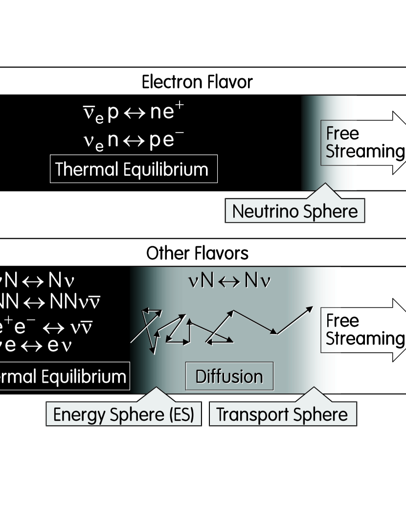
Figure 1: Schematic picture of neutrino spectra formation in the atmosphere of a SN core.

The other flavors interact with the medium primarily by neutral-current collisions on nucleons $\nu N\leftrightarrow N\nu$, a reaction which is sub-dominant for the electron flavor. The nucleon mass $m=938~{}{\rm MeV}$ is much larger than the relevant temperatures which are around $T=10~{}{\rm MeV}$ so that energy exchange between neutrinos and nucleons is inefficient. However, nucleon-nucleon bremsstrahlung $NN\leftrightarrow NN\nu\bar{\nu}$ as well as the leptonic processes $e^{+}e^{-}\leftrightarrow\nu\bar{\nu}$ and $\nu e\leftrightarrow e\nu$ allow for the exchange of energy and the creation or destruction of neutrino pairs and thus keep neutrinos in local thermal equilibrium up to a radius where these reactions freeze out, the “energy sphere.” However, the neutrinos are still trapped by $\nu N\leftrightarrow N\nu$ up to the “transport sphere” whence they stream freely. Between the energy and transport spheres, neutrinos propagate by diffusion. This region plays the role of a scattering atmosphere.

In all numerical simulations of SN neutrino transport the neutrino collisions in the scattering atmosphere were treated as iso-energetic so that the energy $\epsilon_{2}$ of the outgoing neutrino in $\nu N\to N\nu$ was set equal to the energy $\epsilon_{1}$ of the initial state. The main motivation for this approximation was its numerical simplicity and the lack of a compelling interest in details of the emerging $\nu_{\mu}$ and $\nu_{\tau}$ spectra. It is clear, however, that iso-energetic collisions are not a particularly good approximation. In Fig. 2 we show the distribution of final-state energies $\epsilon_{2}$ when $\epsilon_{1}=30~{}{\rm MeV}$ and the medium temperature is $10~{}{\rm MeV}$. A typical nucleon velocity is then about 20% of the speed of light so that it is not surprising that even after a single collision the neutrino energy is considerably smeared out. Since neutrinos interact many times in the scattering atmosphere, and since the medium temperature decreases between the energy and transport spheres, there can be a significant downward adjustment of the neutrino energies (Janka et al. 1996; Hannestad & Raffelt 1998). The main purpose of the present paper is to provide a conceptual understanding and a quantitative estimate of the magnitude of this effect.

Figure 2: Distribution of final-state energies $\epsilon_{2}$ of a neutrino with initial energy $\epsilon_{1}=30~{}{\rm MeV}$, scattering on non-degenerate nucleons in thermal equilibrium with $T=10~{}{\rm MeV}$. Details of how to calculate this plot are described in Appendix B.1.

To address this problem we simplify the model of Fig. 1. The very concept of an “energy sphere” suggests that one should think of it as a source of thermal neutrinos which subsequently diffuse through the scattering atmosphere. Taking this concept literally amounts to the simple picture illustrated in Fig. 3. One no longer worries about detailed processes like $NN$ bremsstrahlung to thermalize the neutrinos, but directly feeds a thermal flux into the scattering atmosphere.

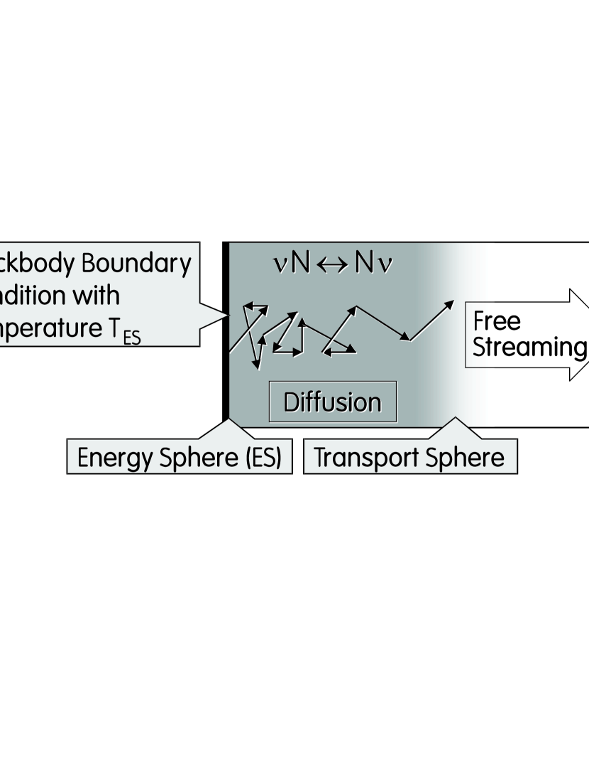
Figure 3: Schematic picture of our simplified treatment of the scattering atmosphere. $T_{\rm ES}$ is the medium temperature at the energy sphere.

Section II of our paper is devoted to showing that this simple picture actually provides a surprisingly accurate representation of the spectra formation problem. The neutrinos streaming off the transport sphere then have fluxes and spectra which depend only on the temperature $T_{\rm ES}$ and the thermally averaged transport optical depth $\bar{\tau}_{\rm ES}$ at the energy sphere which here coincides with the bottom of the scattering atmosphere.

As a next step in Section III we study a scattering atmosphere with a blackbody boundary condition at the bottom and with iso-energetic $\nu N$ collisions as the only neutrino interaction channel. We derive an explicit relationship between $T_{\rm ES}$ and the spectral flux temperature $T_{\rm flux}$ of the escaping neutrinos as a function of $\bar{\tau}_{\rm ES}$. Comparing with full-scale numerical simulations indicates that this exceedingly simple model accounts for the main features of the $\nu_{\mu}$ and $\nu_{\tau}$ spectra.

Then in Section IV we include nucleon recoils in this model. We consider different types of temperature profiles to estimate the shift of the flux temperature and identify the critical parameters which govern $\Delta T_{\rm flux}$.

In Section V we summarize and discuss our findings. Many technical details, especially regarding our implementation of neutrino-nucleon interactions with recoil energy transfer and $NN$ bremsstrahlung, are documented in a series of Appendices.

2 Energy Sphere as a Blackbody Surface

The neutrino sphere, transport sphere, or energy sphere are only approximate concepts because of the energy dependence of the neutrino cross sections. Still, we presently argue that the concept of the energy sphere as a well-defined blackbody surface at the bottom of the scattering atmosphere is much better suited to understand the neutrino spectra than one may have hoped.

To get started we study a practical example. We have performed a $\nu_{\mu}$ and $\nu_{\tau}$ transport calculation with the simple Monte Carlo code described in Appendix E. We use plane-parallel geometry with the medium temperature and density following the power laws

$$\rho=\rho_{0}\,\left(\frac{r_{0}}{r}\right)^{p}\quad\hbox{and}\quad T=T_{0}\,\left(\frac{r_{0}}{r}\right)^{q},$$ (1)

where for the present example $p=10$ and $q=10/4$. The other parameters are $r_{0}=10~{}{\rm km}$, $\rho_{0}=2\times 10^{14}~{}{\rm g~{}cm^{-3}}$ and $T_{0}=31.66~{}{\rm MeV}$.

The neutrinos interact by iso-energetic $\nu N$ scattering and by $NN$ bremsstrahlung. This choice of micro-physics is orthogonal to most previous studies which ignored bremsstrahlung, but included $e^{+}e^{-}\leftrightarrow\nu\bar{\nu}$ and $\nu e\leftrightarrow e\nu$. In this traditional approach spectra formation is conceptually even more complicated because the number-changing process $e^{+}e^{-}\leftrightarrow\nu\bar{\nu}$ freezes out more deeply than the energy-changing process $\nu e\leftrightarrow e\nu$ so that in addition to the transport and energy spheres there is a “number sphere” (Suzuki 1989). Later it was recognized that $NN$ bremsstrahlung is more important than $e^{+}e^{-}$ annihilation (Suzuki 1991, 1993). Hannestad & Raffelt (1998), Thompson, Burrows & Horvath (2000), and Burrows et al. (2000) confirm the importance of $NN$ bremsstrahlung. Moreover, Hannestad & Raffelt (1998) find that the freeze-out spheres for bremsstrahlung and for $\nu e\leftrightarrow e\nu$ roughly coincide in their example of a SN core. Burrows et al. (2000) find that the $\nu_{\mu}$ spectrum depends sensitively on the assumed strength of $NN$ bremsstrahlung, suggesting that $\nu_{\mu}$ thermalization is not vastly dominated by $\nu e$ scattering.

Therefore, reducing the thermalization processes to $NN$ bremsstrahlung likely captures the dominant effect. As this process allows for both the change of neutrino number and energy, the concept of an energy sphere or “thermalization depth” is unambiguous, but of course energy dependent. Ignoring $\nu e$ scattering has the additional benefit that it becomes self-consistent to ignore the chemical composition of the medium. While $\nu N$ scattering and $NN$ bremsstrahlung do depend on the chemical composition, this effect is weak for $\nu N$ scattering. While it may be strong for $NN$ bremsstrahlung, the existing calculations of this process are uncertain to perhaps a factor of 2 (see Appendix C) so that one would not gain much by modeling the composition dependence.

Once the micro physics has been fixed it is straightforward to locate the energy sphere by virtue of a classic argument. Assume the neutrinos have only two interaction channels, i.e. iso-energetic scattering with the inverse transport mean free path (mfp) $\lambda_{T}^{-1}$ and a reaction with the mfp $\lambda_{E}^{-1}$ which changes the energy by a large amount and thus leads to quick thermalization. In this situation the optical depth $\int dr\,\lambda_{E}^{-1}$ for energy exchange is not relevant because neutrinos with a large $\lambda_{T}^{-1}$ are trapped and thus have a greater chance of participating in an energy-changing reaction. This reasoning leads to the optical depth for thermalization (Shapiro & Teukolsky 1983)

$$\tau_{\rm therm}(r)=\int_{r}^{\infty}\!\!dr^{\prime}\,\sqrt{\lambda_{E}^{-1}(r^{\prime})\,\left[\lambda_{T}^{-1}(r^{\prime})+\lambda_{E}^{-1}(r^{\prime})\right]}.$$ (2)

The radius $r_{\rm ES}$ of the energy sphere is implied by

$$\tau_{\rm therm}(r_{\rm ES})=\frac{2}{3}.$$ (3)

Averaging $\tau_{\rm therm}$ over a thermal neutrino spectrum at the local medium temperature leads in our example to $r_{\rm ES}=13.14~{}{\rm km}$ for the location of the energy sphere with a temperature $T_{\rm ES}=16~{}{\rm MeV}$.

In order to discuss non-equilibrium neutrino fluxes and spectra we need to characterize the neutrino distribution function by a few intuitive parameters. One is the spectral temperature $T_{*}$ which we define as

$$T_{*}\equiv\frac{\langle\epsilon\rangle}{3}=\frac{\int_{0}^{\infty}d\epsilon\,\epsilon\int_{-1}^{+1}d\mu f(\epsilon,\mu)}{3\int_{0}^{\infty}d\epsilon\int_{-1}^{+1}d\mu f(\epsilon,\mu)}.$$ (4)

Here, $f(\epsilon,\mu)$ is the neutrino distribution function with $\epsilon$ the energy and $\mu$ the cosine of the angle between the neutrino momentum and the radial direction. (Even for our plane-parallel geometry we will often say “radial” when we mean perpendicular to the medium layer.) We always ignore Pauli blocking, i.e. the Fermi-Dirac nature of neutrinos. The Boltzmann collision equation is then linear in $f$, a considerable numerical simplification which is justified because the $\nu_{\mu}$ and $\nu_{\tau}$ distributions do not have chemical potentials in a SN core. Moreover, in the scattering atmosphere their distribution function is diluted, further reducing the relevance of phase-space blocking. For our study the simplification of ignoring blocking effects far outweighs the small loss of precision. Boltzmann statistics implies that in equilibrium neutrinos follow the distribution function $f=e^{-\epsilon/T}$ so that $\langle\epsilon\rangle=3T$. Inverting this relationship for the non-equilibrium case leads to our definition of $T_{*}$.

In Fig. 4 we show the $T_{*}$ profile for our example as a solid line. (The slight wiggles arise from the limited statistics of the numerical Monte Carlo calculation.) We observe that $T_{*}$ coincides with the medium temperature $T_{\rm med}$ up to the energy sphere; for larger radii the two curves separate. $T_{*}$ still drops considerably until it reaches an asymptotic value which is about half of the energy-sphere temperature $T_{\rm ES}$. This behavior is understood by the $\epsilon^{2}$ dependence of the scattering cross section which causes higher-energy neutrinos to be trapped more effectively than lower-energy ones. Hence, the escaping neutrino flux must be biased towards lower energies.

Figure 4: Numerical example for $\nu_{\mu}$ and $\nu_{\tau}$ transport as described in the text. The inner boundary condition was at 10 km. The thin dashed lines in the upper panel refer to the case without $NN$ bremsstrahlung where a blackbody boundary condition with $T_{\rm ES}=16~{}{\rm MeV}$ is used at the energy sphere.

Therefore, one should carefully distinguish between the spectral temperature $T_{*}$ as defined in Eq. (4) and the spectral flux temperature

$$T_{\rm flux}\equiv\frac{\int_{0}^{\infty}d\epsilon\,\epsilon\int_{-1}^{+1}d\mu\,\mu\,f(\epsilon,\mu)}{3\int_{0}^{\infty}d\epsilon\int_{-1}^{+1}d\mu\,\mu\,f(\epsilon,\mu)}\,.$$ (5)

This is $\langle\epsilon\rangle/3$ of those neutrinos which actually stream. Note that apart from overall factors $2\pi\int_{-1}^{+1}d\mu\,\mu\,f(\epsilon,\mu)$ represents the particle flux. $T_{\rm flux}$ does not include the isotropic part of the distribution which determines $T_{*}$ when the neutrinos are trapped. At large distances where neutrinos stream freely we have $f(\epsilon,\mu)=0$ for backward directions so that $T_{*}$ and $T_{\rm flux}$ are identical up to small differences caused by the exact angular distribution.

In Fig. 4 we show the $T_{\rm flux}$ profile for our numerical example. At large radii indeed $T_{*}\approx T_{\rm flux}$. Moreover, $T_{\rm flux}$ stays constant throughout the scattering atmosphere because no energy exchange with the medium is possible. Flux conservation in the scattering atmosphere is apparent from the lower panel where we show the particle and energy fluxes which both remain constant from roughly the energy sphere outward.

It appears that the separation of the $T_{*}$ and $T_{\rm med}$ profiles, as well as the saturation of $T_{\rm flux}$ and the particle and energy fluxes all happen within a narrow range of radii around the energy sphere. This observation motivates us to repeat the simulation with the lower boundary now at $r_{\rm ES}$, switching off $NN$ bremsstrahlung entirely, and injecting neutrinos with a thermal spectrum corresponding to $T_{\rm ES}=16~{}{\rm MeV}$, i.e. enforcing a neutrino blackbody surface at $r_{\rm ES}$. The resulting temperature profiles are shown in Fig. 4 as dashed lines. $T_{\rm flux}$ is now strictly horizontal. Likewise, the energy and particle fluxes are now strictly conserved so that their profiles are horizontal lines not shown in this plot.

The $T_{*}$ and $T_{\rm flux}$ profiles are surprisingly close to the previous case where neutrinos thermalized by $NN$ bremsstrahlung. Thus, the concept of an energy sphere as a blackbody surface looks encouragingly well justified.

One reason for the extraordinary “sharpness” of the energy sphere in our example is the unusual behavior of the neutrino absorption rate by inverse $NN$ bremsstrahlung; Eq. (C.3) implies approximately $\lambda_{\rm brems}^{-1}\propto\epsilon^{-1}$. This is one of the few neutrino reaction rates which decrease with energy; the scattering rate $\lambda_{T}^{-1}$ increases as $\epsilon^{2}$. With $\lambda_{T}^{-1}+\lambda_{\rm brems}^{-1}\approx\lambda_{T}^{-1}$ we find that the effective thermalization rate under the integral in Eq. (2) varies as $\epsilon^{1/2}$. Therefore, different energy groups decouple thermally at similar radii.

Another reason for a sharply defined energy-sphere temperature is that the density as a function of radius falls much more steeply than the temperature. Therefore, as a function of optical depth the temperature varies slowly. In our example $\lambda_{T}^{-1}\propto\rho$ and approximately $\lambda_{\rm brems}^{-1}\propto\rho^{2}T^{3}$ so that $(\lambda_{\rm brems}^{-1}\lambda_{T}^{-1})^{1/2}\propto\rho^{3/2}T^{3/2}$ or $\tau_{\rm therm}\propto(r_{0}/r)^{3(p+q)/2-1}$ so that $T\propto\tau_{\rm therm}^{w}$ with $w=2q/[3(p+q)-2]$. In our explicit example this is $T\propto\tau_{\rm therm}^{10/71}$. Therefore, the energy spheres for the different energy groups are at similar temperatures.

We thus expect that a blackbody boundary condition at the bottom of the scattering atmosphere provides us with a reasonably accurate understanding of the $\nu_{\mu}$ and $\nu_{\tau}$ spectra formation problem. On the other hand, for the problem of hydrostatically self-consistent atmospheres with multi-flavor neutrino transport (e.g. Schinder & Shapiro 1983) it would be physically more appropriate to use a prescribed neutrino energy flux from the inner star; the atmosphere would then be allowed to adjust in order to transport exactly this flux. In our study, on the other hand, we always assume a fixed background model where the neutrino fluxes are determined by externally prescribed density and temperature profiles as well as the physical assumptions about their interaction with the medium. In that sense our study is similar in spirit to the Monte-Carlo studies of Janka & Hillebrandt (1989a,b) or the more recent work of Burrows et al. (2000). We do not wish to imply that in a real SN core the neutrino fluxes are determined by the temperature at the base of the scattering atmosphere unless this temperature corresponds to a self-consistent stellar structure.

3 Spectral Modification by the Scattering Atmosphere

3.1 Flux Transmission

In our simple picture where the scattering atmosphere is irradiated by a thermal neutrino flux from below, part of that flux will be reflected, part of it transmitted. The reflected flux will be re-absorbed because a blackbody surface is by definition a perfect absorber. To determine the emerging $\nu_{\mu}$ and $\nu_{\tau}$ flux it is therefore enough to calculate the energy-dependent flux transmission factor, i.e. the fraction of the primary flux that is transmitted without being reflected back into the radiating surface.

For sufficiently low energies the scattering atmosphere is transparent so that the transmission factor is unity. In the opposite limit where the neutrino mfp is short compared with the geometric dimension of the layer (diffusion limit), the Boltzmann collision equation can be solved analytically (Appendix A), leading for a plane-parallel geometry to a transmission ratio of

$$s(\tau_{\rm ES})=\frac{4}{3\tau_{\rm ES}}.$$ (6)

Here, $\tau_{\rm ES}$ is the transport optical depth of the energy sphere

$$\tau_{\rm ES}\equiv\int_{r_{\rm ES}}^{\infty}dr\,n_{B}(r)\int_{-1}^{+1}d\cos\theta\,(1-\cos\theta)\,\frac{d\sigma}{d\cos\theta},$$ (7)

where $n_{B}$ is the number density of scatterers (“baryons”), $d\sigma/d\cos\theta$ the differential scattering cross section, and $r_{\rm ES}$ the lower boundary of the scattering atmosphere, i.e. the energy sphere.

In the intermediate regime $\tau_{\rm ES}={\cal O}(1)$ we solve the Boltzmann collision equation numerically. To do so we have to commit ourselves to a specific form of the differential scattering cross section. We use the “dipole formula” $d\sigma/d\cos\theta=\sigma_{0}\,(1+b\cos\theta)/2$ where $-1\leq b\leq+1$ and the total cross section is $\sigma_{0}$. When expressed in terms of the transport optical depth $\tau_{\rm ES}$, the flux transmission is independent of $b$ for small and large $\tau_{\rm ES}$. For intermediate $\tau_{\rm ES}$ the variation with $b$ is less than $\pm 1\%$, i.e. for all practical intents and purposes it is enough to use the transport optical depth as the only relevant parameter.

The numerical transmission factor for $b=0$ is shown in Fig. 5; for other $b$-values it is within the line-width of this curve. An analytic approximation is

$$s(\tau_{\rm ES}) = \left[1+\frac{3\,\tau_{\rm ES}}{4}\right]^{-1}$$

$$\kern-50.00008pt{}\times\left[1-\frac{0.033}{1+1.5\,(\ell_{\tau}+0.17)^{2}+0.5\,(\ell_{\tau}+0.32)^{6}}\right],$$

where $\ell_{\tau}\equiv\log_{10}(\tau_{\rm ES})$. The first bracket alone overestimates the numerical result by less than 4% in the entire range $0<\tau_{\rm ES}<\infty$. The second bracket improves the approximation to better than $\pm 0.05\%$.

Figure 5: Flux transmission factor for a plane-parallel scattering atmosphere with transport optical depth $\tau_{\rm ES}$.

For a spherically symmetric geometry these results need to be modified. In Appendix A we show that in the diffusion limit the transmission factor is the same as for a plane-parallel geometry, provided one includes a factor $(r_{\rm ES}/r)^{2}$ under the integral in Eq. (7). The resulting quantity $\tau^{*}_{\rm ES}$, of course, is no longer the transport optical depth, but for the purposes of flux transmission it plays an analogous role. For the spherical case we have not investigated the intermediate regime $\tau^{*}_{\rm ES}={\cal O}(1)$, but assume that the plane-parallel interpolation formula Eq. (3.1) applies with reasonable accuracy.

3.2 Spectral Modification

Next we study the flux and spectrum of the transmitted neutrinos if the primary flux is thermal at a temperature $T_{\rm ES}$. We characterize the “thickness” of the plane-parallel scattering atmosphere by $\bar{\tau}_{\rm ES}$, defined as the transport optical depth at the energy sphere, averaged over a Maxwell-Boltzmann spectrum at $T_{\rm ES}$. Taking the scattering cross section to vary as $\epsilon^{2}$ we note that $\langle\epsilon^{2}\rangle=12\,T_{\rm ES}^{2}$ so that $\bar{\tau}_{\rm ES}$ amounts to the transport optical depth at the fixed energy $\epsilon=\sqrt{12}\,T_{\rm ES}\approx 3.4641\,T_{\rm ES}$. Put another way, we use $\tau_{\rm ES}(\epsilon)=(\bar{\tau}_{\rm ES}/12)(\epsilon/T_{\rm ES})^{2}$ to calculate the energy-dependent transmission factor.

In Fig. 7 we show the energy-dependent transmitted flux for several values of $\bar{\tau}_{\rm ES}$. One parameter to characterize these spectra is their flux temperature $T_{\rm flux}$ as defined in Eq. (5). In Fig. 7 we show the same spectra after re-scaling the horizontal axis with the appropriate $T_{\rm flux}$ and normalizing them. This representation shows how closely these functions mimic true thermal spectra.

Figure 6: Transmitted flux for the indicated values of $\bar{\tau}_{\rm ES}$.

Figure 7: Transmitted flux (normalized) for the indicated values of $\bar{\tau}_{\rm ES}$ where the neutrino energy is in units of $T_{\rm flux}$.

The flux temperature $T_{\rm flux}$ in units of $T_{\rm ES}$ as a function of $\bar{\tau}_{\rm ES}$ is shown in the upper panel of Fig. 8. For $\bar{\tau}_{\rm ES}\ll 1$ we have, of course, $T_{\rm flux}=T_{\rm ES}$. In the opposite limit $\bar{\tau}_{\rm ES}\to\infty$ the transmission factor is proportional to $\epsilon^{-2}$ so that the transmitted spectrum is proportional to $e^{-\epsilon/T_{\rm ES}}$ rather than the primary $\epsilon^{2}e^{-\epsilon/T_{\rm ES}}$, implying $T_{\rm flux}=\frac{1}{3}\,T_{\rm ES}$. $T_{\rm flux}$ is significantly smaller than $T_{\rm ES}$ even for relatively small values of $\bar{\tau}_{\rm ES}$. An analytic approximation formula is

$$\frac{T_{\rm flux}}{T_{\rm ES}} = \Biggl{[}\frac{1}{3}+\frac{2}{3\,(1+0.35\,\bar{\tau}_{\rm ES}^{0.53})}\Biggr{]}$$ (9)

$$\times \Biggl{[}1-0.03\,(1-0.75\,y^{2})\,e^{-0.27\,y^{2}}\Biggr{]}$$

where $y=\log_{10}(\bar{\tau}_{\rm ES})-0.9$. The first bracket alone approximates the true result to better than 4% while the second bracket improves the approximation to better than $\pm 0.3\%$ everywhere. To study power-law models it is also useful to have a power-law representation. We find that

$$\frac{T_{\rm flux}}{T_{\rm ES}}=\frac{0.83}{\bar{\tau}_{\rm ES}^{0.128}}$$ (10)

works well in the range $1\lesssim\bar{\tau}_{\rm ES}\lesssim 100$ (dashed line in the upper panel of Fig. 8).

Figure 8: Spectral characteristics of the transmitted flux.

The deviation of the spectrum from a thermal shape may be characterized by the “pinching parameter”

$$p\equiv\frac{3}{4}\,\frac{\langle\epsilon^{2}\rangle}{\langle\epsilon\rangle^{2}}$$ (11)

where $p=1$ for a Maxwell-Boltzmann spectrum. If the high- and low-energy parts of the spectrum are relatively suppressed, the spectrum is called “pinched” ($p<1$), in the opposite case “anti-pinched” ($p>1$). The limiting cases are $p=1$ for $\bar{\tau}_{\rm ES}\to 0$ and $\frac{3}{2}$ for $\bar{\tau}_{\rm ES}\to\infty$. Intermediate values are shown in Fig. 8 and Table 1.

Table 1: Spectral modification of neutrino flux.

$\bar{\tau}_{\rm ES}$	$T_{\rm flux}/T_{\rm ES}$	$p$	$\phi$
0	1	1	1
1	0.82	0.99	1.18
3	0.72	1.01	1.17
10	0.62	1.05	1.04
30	0.54	1.10	0.79
100	0.47	1.17	0.49
$\infty$	1/3	3/2	0

The concept of spectral pinching refers to the width of the energy distribution. Therefore, another choice for the pinching parameter might have been something like $(\langle\epsilon^{2}\rangle-\langle\epsilon\rangle^{2})/\langle\epsilon\rangle^{2}$. This definition is equivalent to $p$ aside from a shift of the zero point and the normalization. Either way one uses the quadratic moment $\langle\epsilon^{2}\rangle$ in addition to $\langle\epsilon\rangle$ to characterize the spectrum.

In the literature, non-thermal SN neutrino spectra are often described by a degeneracy parameter $\eta$. This representation has the disadvantage that anti-pinched spectra are not covered because the limit $\eta\to-\infty$ represents a Boltzmann distribution.

A further characteristic of the transmitted flux is its luminosity. It may be larger or smaller than given by the Stefan-Boltzmann law in terms of $T_{\rm flux}$. We call the ratio of the true luminosity relative to this Stefan-Boltzmann value the “greyness factor” $\phi$. When $\phi<1$ the transmitted flux is “grey” in that it carries less energy than a blackbody flux of the same spectral shape. In the bottom panel of Fig. 8 we show $\phi$; some values are given in Table 1.

If the scattering atmosphere is very thick ($\bar{\tau}_{\rm ES}\gg 1$) the emerging spectrum approaches a limiting spectral temperature of $\frac{1}{3}T_{\rm ES}$ as explained above Eq. (9), while the flux is arbitrarily diluted. Therefore, the greyness factor will become arbitrarily small. It is remarkable, however, that $\phi=1$ within $\pm 20\%$ for $\bar{\tau}_{\rm ES}$ as large as 30. Therefore, if in realistic examples of density and temperature profiles the energy sphere is at $\bar{\tau}_{\rm ES}<30$, then the emerging flux will be surprisingly close to a Stefan-Boltzmann flux as calculated with the spectral temperature $T_{\rm flux}$. Put another way, for $\bar{\tau}_{\rm ES}<30$ the overall flux dilution and spectral shift conspire to mimic the Stefan-Boltzmann law for the emerging flux. This unintuitive behavior is a consequence of the $\epsilon^{2}$ dependence of the transport cross section. If the cross section were energy independent, then the flux would be diluted without a spectral shift, and even for small $\bar{\tau}_{\rm ES}$ the emerging flux would appear diluted (grey) relative to its spectral temperature.

The neutrino fluxes and spectra from SN cores are usually described as showing equipartition of energy between different flavors, yet a hierarchy of spectral temperatures. At late times when the star is settled and the density and temperature profiles in the atmosphere are steep, the radiating surfaces for different flavors are similar. Therefore, as stressed by Janka (1995), similar luminosities with different spectral temperatures must be explained by the flux dilution caused by the scattering atmosphere. Janka (1995) did not worry about the spectral shift caused by the $\epsilon^{2}$ variation of the transport cross section so that his conclusions would have applied to any optical depth of the energy sphere. Our more refined treatment suggests that large spectral differences and similar luminosities for the different flavors at late times require average optical depths of the $\nu_{\mu}$ energy sphere exceeding about $30$. However, it is precisesly at late times when $Y_{e}$ is small and the density gradients are steep that the $NN$ bremsstrahlung process is likely to dominate over the leptonic processes. Once $NN$ bremsstrahlung is included in future numerical simulations it remains to be seen if at late times the energy sphere moves to such large optical depths as to cause significantly “grey” $\nu_{\mu}$ or $\nu_{\tau}$ fluxes.

In summary, for values of $\bar{\tau}_{\rm ES}$ up to 30 the transmitted flux resembles a thermal spectrum in both its absolute flux as well as its spectral shape. However, the relevant temperature is not $T_{\rm ES}$, but rather a reduced temperature $T_{\rm flux}$. For $\bar{\tau}_{\rm ES}=10$–30 we find $T_{\rm flux}/T_{\rm ES}=0.62$–0.54. Therefore, we expect that the $\nu_{\mu}$ and $\nu_{\tau}$ flux from a SN core is roughly thermal with a temperature $T_{\rm flux}\approx 0.6\,T_{\rm ES}$ and a luminosity given approximately by the Stefan-Boltzmann law, taking $T_{\rm flux}$ for the temperature and the area of the energy sphere for the radiating surface. Only for $\bar{\tau}_{\rm ES}<30$ is the emerging flux significantly diluted below the Stefan-Boltzmann level corresponding to its spectral temperature $T_{\rm flux}$.

Figure 9: SN model for the Monte Carlo transport study of Janka & Hillebrandt (1989b), Model II.

Figure 10: SN model 324 ms after bounce from a Newtonian calculation (Messer et al. 2001).

3.3 Comparing with Full-Scale Simulations

3.3.1 Janka & Hillebrandt (1989b) Model

As a “reality check” on our explanation of $\nu_{\mu}$ and $\nu_{\tau}$ spectra we turn to comparing our predictions with full-scale numerical simulations in the literature. As a first case we consider the Monte Carlo transport simulations of Janka & Hillebrandt (1989a,b) where the multi-flavor neutrino fluxes were calculated on the basis of a fixed background model. This model consisted of ten radial zones, each 12 km wide; in Fig. 9 we show the temperature and density profiles. (I thank Thomas Janka for providing these profiles.) The local $\nu_{\mu}$ and $\nu_{\tau}$ temperature $T_{*}$ found in this Monte Carlo simulation is indicated by filled circles in the third panel of Fig. 9; the flux temperature $T_{\rm flux}$ by open circles. As expected, $T_{*}$ and $T_{\rm flux}$ coincide for large radii, but are vastly different in regions where the neutrinos still scatter.

In the second panel of Fig. 9 we show the average transport optical depth $\bar{\tau}$. To this end we calculate the transport optical depth, modified for the spherical case, and average it thermally with the local medium temperature. For the transport opacity we use Eq. (B.1) which ignores the vector-current contribution and also ignores nucleon degeneracy effects, two approximations which work in opposite directions, and anyway, are small corrections for the situation at hand.

On the basis of this $\bar{\tau}(r)$ and $T_{\rm med}(r)$ we calculate for each radius the predicted flux temperature $T_{\rm flux}(r_{\rm ES})$ of the escaping neutrino flux if the energy sphere were at that radius. This is the lowest curve in the third panel of Fig. 9. The actual $T_{\rm flux}$ at large radii found in the Monte Carlo study is shown as a horizontal dotted line in the third panel. It intersects the $T_{\rm flux}(r_{\rm ES})$ curve at a radius of about 50 km, indicated by a vertical dotted line. This radius is $r_{\rm ES}$ if our picture is correct. We note that at $r_{\rm ES}=50~{}{\rm km}$ we have $\bar{\tau}\approx 10$.

The neutrino temperature $T_{*}$ (top curve in the third panel) separates from $T_{\rm med}$ at about the same radius so that it is consistent to interpret 50 km as $r_{\rm ES}$.

Likewise, the numerical particle flux shown in the fourth panel reaches its asymptotic value at about the same radius so that, indeed, the energy sphere must be around 50 km. Within our simple picture we can also predict the particle flux, assuming that the energy sphere is at a given radius. This prediction is shown as a thin line in the fourth panel. If $r_{\rm ES}=50~{}{\rm km}$ we would predict that a neutrino flux of about $3.5\times 10^{57}~{}{\rm s}^{-1}$ is emitted from this SN model. Comparing this with the Monte Carlo result of $2.6\times 10^{57}~{}{\rm s}^{-1}$, the agreement is not too bad.

In this numerical study the only number-changing reaction was $e^{+}e^{-}\leftrightarrow\nu\bar{\nu}$, for energy exchange there was also $\nu e\leftrightarrow e\nu$. As these processes may freeze out at different radii, the simple picture of one energy sphere is certainly not entirely adequate. Therefore, it is quite surprising how well our simple description can account for the main features of the Monte Carlo results.

3.3.2 Messer et al. (2001) Model

As a second case we apply the same analysis to a model of Messer et al. (2001), provided to us by B. Messer. It is based on a full-scale Newtonian collapse simulation of the Woosley & Weaver $15\,M_{\odot}$ progenitor model labelled s15s7b, calculated with the SN code described by Mezzacappa et al. (2001). We use a snapshot at 324 ms after bounce when the shock wave is at a radius of about 120 km, i.e. the SN core still accretes matter. We plot in Fig. 10 the radial profile of the density, medium temperature, $\nu_{\mu}$ temperatures $T_{*}$ and $T_{\rm flux}$, particle flux, and luminosity (energy flux). Proceeding as before, we find that the energy sphere should be at about 25 km (vertical dotted line) and that $\bar{\tau}(r_{\rm ES})\approx 40$. The main conclusions are the same as in the previous example.

Our simple model for the $\nu_{\mu}$ and $\nu_{\tau}$ spectra apparently works so well because the predicted flux temperature is rather insensitive to the assumed location of the energy sphere. From the particle and energy fluxes in the bottom panel of Fig. 10 one might have located the energy sphere, say, anywhere in the range $r_{\rm ES}=23$–29 km. One still would have predicted $T_{\rm flux}$ within $\pm 10\%$ of the numerical value. Our approach of representing the energy sphere by a blackbody surface looks like a robust approximation.

3.4 Is $NN$ Bremsstrahlung Really Important?

Within these specific models we can return to the question if nucleonic bremsstrahlung $NN\leftrightarrow NN\nu\bar{\nu}$ is really important relative to the leptonic processes that were actually included in these simulations. Based on the bremsstrahlung process alone we have calculated the thermalization depth $\bar{\tau}_{\rm therm}$ as defined in Eq. (2), averaged over a thermal spectrum with the local medium temperature. For simplicity we have used the bremsstrahlung rate as in Eq. (C.3) with $B(x)=1$. We show $\bar{\tau}_{\rm therm}$ as the lower curve in the second panel of Figs. 9 and 10.

In the Janka & Hillebrandt (1989b) model $\bar{\tau}_{\rm therm}\ll 1$ at the location of the energy sphere so that bremsstrahlung would have been unimportant even if it had been included. Bremsstrahlung depends on $\rho^{2}$ and thus drops quickly in low-density regions. This SN atmosphere has rather low densities so that it is not surprising that $NN$ bremsstrahlung is unimportant.

In the Messer et al. (2001) model the actual energy sphere is close to the bremsstrahlung thermalization sphere, i.e. the radius where the lower curve in the second panel is 2/3. Therefore, in this model $NN$ bremsstrahlung would have been roughly competitive with the leptonic processes that actually were included. Note that the density at the energy sphere is about 10 times larger than in the Janka & Hillebrandt (1989b) case.

In these models the atmospheres are still dominated by accretion. After a successful explosion they will settle to more compact dimensions, presumably enhancing the role of $NN$ bremsstrahlung. We note that the model used by Hannestad & Raffelt (1998) represented a settled proto neutron star so that their finding of the importance of bremsstrahlung is not inconsistent with the present discussion. Apparently it depends on the detailed atmospheric structure which processes predominate for the $\nu_{\mu}$ and $\nu_{\tau}$ thermalization.

3.5 Sensitivity of $T_{\rm flux}$ to Thermalization Process

We may explicitly test the sensitivity of the predicted flux temperature $T_{\rm flux}$ to the strength of the assumed thermalization process by means of a power-law model of the stellar atmosphere as in Eq. (1), i.e. $\rho\propto r^{-p}$ and $T\propto r^{-q}$. For the scattering and energy-exchange rates we assume

$$\lambda_{T}^{-1} \propto \rho\,\epsilon^{2}\propto r^{-p}\,\epsilon^{2},$$

$$\lambda_{E}^{-1} \propto \beta\,\rho^{u}\,T^{v}\,\epsilon^{w}\propto\beta r^{-up-vq}\,\epsilon^{w},$$ (12)

where for $NN$ bremsstrahlung approximately $u=2$, $v=3$ and $w=-1$. Further, $\beta$ is a fudge factor which allows us to adjust the strength of the energy-exchange process. The thermalization rate then scales as

$$\left(\lambda_{T}^{-1}\lambda_{E}^{-1}\right)^{1/2}\propto\beta^{1/2}\,r^{-x}\,\epsilon^{y}$$ (13)

with $x=\frac{1}{2}[(u+1)p+vq]$ and $y=\frac{1}{2}(2+w)$. Finally, according to Eq. (10) we use

$$T_{\rm flux}\propto T_{\rm ES}\,\bar{\tau}_{\rm ES}^{-t}$$ (14)

with $t=0.128$.

It is now a matter of simple integrations to show that the transport optical depth and thermalization depth scale as $\tau\propto r^{-(p-1)}\,\epsilon^{2}$ and $\tau_{\rm therm}\propto\beta^{1/2}\,r^{-(x-1)}\,\epsilon^{y}$. The local thermal averages of the energy expressions are $\langle\epsilon^{2}\rangle\propto T^{2}\propto r^{-2q}$ and $\langle\epsilon^{y}\rangle\propto T^{y}\propto r^{-yq}$ so that the thermally averaged optical depths are

$$\bar{\tau} \propto r^{-(p+2q-1)},$$

$$\bar{\tau}_{\rm therm} \propto \beta^{1/2}\,r^{-(x+yq-1)}.$$ (15)

The energy sphere is located where $\bar{\tau}_{\rm therm}=2/3$ so that

$$r_{\rm ES}\propto\beta^{\textstyle\frac{1}{2(x+yq-1)}}$$ (16)

Therefore, the optical depth and temperature at the energy sphere scale as

$$T_{\rm ES} \propto \beta^{-\textstyle\frac{q}{2(x+yq-1)}},$$

$$\bar{\tau}_{\rm ES} \propto \beta^{-\textstyle\frac{p+2q-1}{2(x+yq-1)}}.$$ (17)

Finally, with Eq. (14) we find

$$T_{\rm flux}\propto\beta^{z}$$ (18)

with

$$z=\frac{t(p+2q-1)-q}{2(x+yq-1)}.$$ (19)

If $NN$ bremsstrahlung is the thermalization process this translates into

$$z_{\rm brems}=\frac{t(p+2q-1)-q}{3p+4q-2}.$$ (20)

Since typically the density and temperature gradients are steep, dropping the $-1$ and $-2$ terms will introduce only a small error so that

$$z_{\rm brems}=\frac{t(1+2q/p)-q/p}{3+4q/p}.$$ (21)

Noting that typically we will have $q/p=0.25$–0.35 we find that $z_{\rm brems}$ is between $-0.015$ and $-0.105$. Taking this latter number as typical, a factor of 3 uncertainty in the bremsstrahlung rate translates roughly into a 10% uncertainty of the predicted $T_{\rm flux}$. Of course, this estimate depends on the temperature and density profile remaining unchanged by the variation of $\beta$; a self-consistent treatment is not possible with the present approach.

3.6 Flavor Dependence of Spectral Temperature

We may also address the question of the relative spectral flux temperature between $\bar{\nu}_{e}$ or $\nu_{e}$ and the other flavors for the case of a recoil-free scattering atmosphere. To this end we must specify temperature and density profiles of the medium which we choose as power laws of the form Eq. (1) with $T_{0}$, $r_{0}$ and $\rho_{0}$ the energy-sphere values. For a plane-parallel geometry, the medium temperature profile as a function of the transport optical depth $\tau(\epsilon)$ for a given neutrino energy $\epsilon$ is easily found to be

$$\frac{T_{\rm med}}{T_{\rm ES}}=\left(\frac{12\,T_{\rm ES}^{2}\,\tau(\epsilon)}{\epsilon^{2}\,\bar{\tau}_{\rm ES}}\right)^{u}$$ (22)

with $u=q/(p-1)$. If the density falls steeply so that $p\gg 1$ we have $u\approx q/p$. Realistic values for this power-law index are in the range, say, $u=0.25$–0.35.

For a given energy $\epsilon$ the $\nu_{e}$ or $\bar{\nu}_{e}$ decouple at their respective energy spheres. The main energy-exchange process relevant for these species are charged-current (CC) processes involving electrons or positrons such as $\bar{\nu}_{e}+p\leftrightarrow n+e^{+}$. In addition there are neutral-current (NC) elastic collisions on nucleons. Since both CC and NC processes have the same $\epsilon^{2}$ behavior we may write $\lambda_{\rm CC}^{-1}=\xi\lambda_{\rm NC}^{-1}$ with $\xi$ a factor which depends on the medium’s composition and the degree of electron and nucleon degeneracy. Moreover, $\xi$ is different for $\nu_{e}$ and $\bar{\nu}_{e}$. In the absence of degeneracy effects we have $\xi_{\nu_{e}}\approx 4\,(1-Y_{e})$ and $\xi_{\bar{\nu}_{e}}\approx 4\,Y_{e}$ where $Y_{e}$ is the electron fraction per baryon. Note that the CC cross section is roughly 4 times the NC one and that only neutrons are available as CC targets for $\nu_{e}$, and only protons for $\bar{\nu}_{e}$. We now apply the Shapiro-Teukolsky criterion Eq. (2) and find that the energy-dependent mfp for thermalization is $\lambda_{\rm therm}^{-1}=(\lambda_{\rm CC}^{-1}\lambda_{\rm NC}^{-1})^{1/2}=[\xi(1+\xi)]^{1/2}\,\lambda_{\rm NC}^{-1}$. Integrating over radius to obtain the optical depth then yields $\tau_{\rm therm}(\epsilon)=[\xi(1+\xi)]^{1/2}\tau(\epsilon)$ where $\tau(\epsilon)$ is the NC transport optical depth. The energy-dependent energy sphere is then located where $\tau_{\rm therm}(\epsilon)=2/3$ so that the NC transport optical depth at this location is $\tau(\epsilon)=(2/3)[\xi(1+\xi)]^{-1/2}$. The above profile then informs us that

$$\frac{T_{\epsilon}}{T_{\rm ES}}=\left(\frac{8}{\bar{\tau}_{\rm ES}\sqrt{\xi(1+\xi)}}\right)^{u}\left(\frac{T_{\rm ES}}{\epsilon}\right)^{2u}$$ (23)

is the medium temperature at the energy dependent energy spheres for $\nu_{e}$ or $\bar{\nu}_{e}$.

The main assumption for calculating the $\nu_{e}$ or $\bar{\nu}_{e}$ spectra is that every energy group is emitted with a thermal flux corresponding to $T_{\epsilon}$, i.e. we ignore chemical-potential effects. The escaping spectrum is then proportional to $\epsilon^{2}\,e^{-\epsilon/T_{\epsilon}}$. Note that every energy group is at the same transport optical depth because both NC and CC processes have the same energy dependence. (For every energy group the energy sphere is at $\tau_{\rm therm}(\epsilon)=2/3$ so that this location also corresponds to a common value for the transport optical depth.) Therefore, the flux dilution caused by NC scatterings does not modulate the spectral shape.

It is now a simple matter of integration to determine the $\nu_{e}$ or $\bar{\nu}_{e}$ flux temperature and pinching parameter,

$$T_{{\rm flux},\nu_{e}} = \left(\frac{8}{\bar{\tau}_{\rm ES}\sqrt{\xi(1+\xi)}}\right)^{\textstyle\frac{u}{1+2u}}\frac{\Gamma\left(\frac{5+2u}{1+2u}\right)}{\Gamma\left(\frac{4+2u}{1+2u}\right)},$$

$$p_{\nu_{e}} = \frac{4\,\Gamma\left(\frac{4+2u}{1+2u}\right)\Gamma\left(\frac{6+2u}{1+2u}\right)}{5\left[\Gamma\left(\frac{5+2u}{1+2u}\right)\right]^{2}},$$ (24)

where $\Gamma$ is the Gamma function. These spectra are always pinched because $p<1$ for $u\geq 0$. Around the realistic value $u=0.3$ we find the expansion

$$T_{{\rm flux},\nu_{e}} \approx \left(\frac{8}{\bar{\tau}_{\rm ES}\sqrt{\xi(1+\xi)}}\right)^{0.19+\Delta u}$$

$$\times \bigl{(}0.465-0.65\,\Delta u\bigr{)},$$

$$p_{\nu_{e}} \approx 0.911-0.18\,\Delta u,$$ (25)

where $\Delta u\equiv u-0.3$.

As a first consequence we can estimate the relative spectral temperature between $\nu_{e}$ and $\bar{\nu}_{e}$,

$$\frac{T_{{\rm flux},\nu_{e}}}{T_{{\rm flux},\bar{\nu}_{e}}}=\left(\frac{4Y_{e}(4Y_{e}+1)}{4(1-Y_{e})[4(1-Y_{e})+1]}\right)^{\frac{u}{2(1+2u)}}.$$ (26)

For $u=0.3$ and to lowest order in $Y_{e}$ this is $0.69\,(Y_{e}/0.1)^{0.094}$, in the ball park of what is found in numerical simulations.

With the power-law representation of the $\nu_{\mu}$ flux temperature of Eq. (10) we find

$$\frac{T_{{\rm flux},\nu_{\mu}}}{T_{{\rm flux},\nu_{e},\bar{\nu}_{e}}} \approx \Bigl{(}1.39+1.9\,\Delta u\Bigr{)}$$ (27)

$$\times [\xi(1+\xi)]^{0.094+0.2\,\Delta u}$$

$$\times \left(\frac{\bar{\tau}_{\rm ES}}{10}\right)^{0.06+0.4\,\Delta u}.$$

For $\bar{\nu}_{e}$ we have $\xi(1+\xi)=4Y_{e}(1+4Y_{e})$. Thus for small $Y_{e}$ we have to lowest order

$$\frac{T_{{\rm flux},\bar{\nu}_{\mu}}}{T_{{\rm flux},\bar{\nu}_{e}}} \approx \Bigl{(}1.32+1.8\,\Delta u\Bigr{)}$$ (28)

$$\times (Y_{e}/0.1)^{0.094+0.2\,\Delta u}$$

$$\times \left(\frac{\bar{\tau}_{\rm ES}}{10}\right)^{0.06+0.4\,\Delta u}.$$

This ratio is almost independent of the optical depth of the $\nu_{\mu}$ energy sphere; changing $\bar{\tau}_{\rm ES}$ by a factor of 2 modifies the temperature ratio by around 5%. A change $\Delta u=0.05$ implies a 7% modification of the temperature ratio. Finally, changing $Y_{e}$ by a factor of 2 causes something like a 7% modification.

In deriving this result we have made several simplifying assumptions so that the final answer should not be overinterpreted. Still, it is gratifying that our simple model, without any fine-tuning, reproduces relative neutrino flux temperatures which fully concur with what is found in numerical simulations. This finding, again, encourages us to put some faith in our explanation of the SN neutrino spectra.

4 Nucleon Recoils

4.1 First Example

We now turn to the main goal of our investigation, the effect of including nucleon recoils in the scattering atmosphere. To illustrate the type and magnitude of effect to be expected we begin with the same plane-parallel power-law model that was shown in Fig. 4, except that now we allow for recoil energy transfers in $\nu N$ collisions according to the formalism described in Appendix B. The resulting radial runs of parameters are shown in Fig. 11

Figure 11: Example of Fig. 4 with nucleon recoils included. The thin dashed lines refer to the case with a blackbody boundary condition $T_{\rm ES}=16~{}{\rm MeV}$ at the energy sphere. The long-dashed line is $T_{*}$ for the no-recoil case of Fig. 4.

Nucleon recoils cause the neutrino temperature $T_{*}$ to follow more closely the medium; the no-recoil case is shown as a long-dashed line. The $T_{\rm flux}$ profile is shifted downward so that the neutrinos emerge with a lower $T_{\rm flux}$ at the surface. The luminosity profile has a “bump” near the energy sphere, indicating that the neutrinos transfer energy to the medium within the scattering atmosphere.

The energy sphere shown here is the same as in Fig. 11, i.e. strictly speaking we mean the thermalization depth of $NN$ bremsstrahlung when we say “energy sphere.” Of course, in the present situation the concept of an energy sphere no longer applies in the sense that nucleon recoils allow for energy transfers throughout the scattering atmosphere, which in turn no longer is strictly a scattering atmosphere.

Next, we switch off $NN$ bremsstrahlung entirely and use a blackbody boundary condition with $T_{\rm ES}=16~{}{\rm MeV}$ at $r_{\rm ES}$. The resulting profiles are shown as short-dashed thin lines. We practically obtain the same $T_{*}$ and $T_{\rm flux}$ profiles whether we allow the neutrinos to thermalize by $NN$ bremsstrahlung or if we enforce a blackbody surface at $r_{\rm ES}$, confirming our previous arguments.

This approach has one more advantage. In general, $\Delta T_{\rm flux}$ depends on both the density and temperature profiles of the scattering atmosphere. However, if $\nu N$ scattering is the only remaining process, then the only natural measure of distance is the transport optical depth $\tau$. Put another way, the medium density disappears from the Boltzmann collision equation if we use a quantity proportional to $\int dr\,n_{B}(r)$ as a radial coordinate. For us it is most practical to use the transport optical depth, averaged over a thermal neutrino spectrum at $T_{\rm ES}$. Note that we use the same thermal average everywhere so that the $T_{\rm med}$ profile does not enter the transformation from $r$ to $\bar{\tau}$. Then the only relevant profile is $T_{\rm med}(\bar{\tau})$.

Figure 12: Same as Fig. 11, except with the optical depth as the radial coordinate.

Therefore, radial profiles such as Fig. 11 are actually plotted in the “wrong” coordinate for issues related to neutrino transport. For illustration we show the same profiles in Fig. 12 with $\bar{\tau}$ as the radial coordinate, scaled to $\bar{\tau}_{\rm ES}$. We recognize that all temperature profiles vary slowly in the neighborhood of the energy sphere.

The “bump” in the luminosity profile turns out to extend throughout the scattering atmosphere. For the blackbody boundary condition, the luminosity decreases nearly linearly toward the surface so that the neutrinos transfer energy to the medium throughout the scattering atmosphere with approximately the same rate everywhere. It is interesting that the luminosity profiles are very different between the $NN$-thermalization case and that with a blackbody boundary condition.

4.2 Constant Temperature

Turning to a systematic study of the impact of nucleon recoils we consider a scattering atmosphere with a fixed temperature $T_{\rm med}$, whereas the blackbody surface at the bottom is at the temperature $T_{\rm ES}\geq T_{\rm med}$. What is the spectrum of the emerging neutrinos?

Actually not even the sign of $\Delta T_{\rm flux}$ caused by nucleon recoils is a priori obvious. Since $T^{0}_{\rm flux}<T_{\rm ES}$ it is conceivable that energy exchange will increase $T_{\rm flux}$ in a situation when $T_{\rm med}>T^{0}_{\rm flux}$. (The superscript 0 refers to the no-recoil case.) Conversely, one expects the energies of the emerging neutrinos to be lowered when $T_{\rm med}<T^{0}_{\rm flux}$.

The real answer is more complicated. In Fig. 13 we show the $T_{*}$ and $T_{\rm flux}$ profiles for a scattering atmosphere with $\bar{\tau}_{\rm ES}=100$ and $T_{\rm ES}=20~{}{\rm MeV}$. The dashed lines are for the no-recoil case. The three panels are for the different medium temperatures 20, 12, and 4 MeV as indicated by dotted lines.

Figure 13: Neutrino temperature profiles $T_{*}$ and $T_{\rm flux}$ for $T_{\rm ES}=20~{}{\rm MeV}$ and $T_{\rm med}=20$, 12 and $4~{}{\rm MeV}$ (top to bottom). Dashed lines for the no-recoil case, dotted lines for $T_{\rm med}$.

Figure 14: Neutrino temperature profiles $T_{*}$ and $T_{\rm flux}$ for $T_{\rm ES}=20~{}{\rm MeV}$. From top to bottom the curves are for $T_{\rm med}=20$ to 2 MeV in steps of 2 MeV. Dashed lines are for the no-recoil case.

Figure 15: Variation of neutrino flux parameters at the surface with medium temperature for several values of $\bar{\tau}_{\rm ES}$.

In the first panel where $T_{\rm med}=T_{\rm ES}$ the trapped neutrinos approach more closely $T_{\rm med}$, while $T_{\rm flux}$ at the surface actually increases! In the second panel we use $T_{\rm flux}^{0}<T_{\rm med}<T_{\rm ES}$. The $T_{*}$ profile is close to $T_{\rm med}$ while $T_{\rm flux}$ shoots up near the energy sphere. However, in spite of $T_{\rm flux}^{0}<T_{\rm med}$, at the surface $T_{\rm flux}$ reaches a value below the no-recoil case. The overall behavior is similar in the third panel where $T_{\rm med}<T_{\rm flux}^{0}<T_{\rm ES}$.

In Fig. 14 we show the $T_{*}$ and $T_{\rm flux}$ profiles for $T_{\rm med}$ varying from $T_{\rm ES}=20~{}{\rm MeV}$ to 2 MeV in steps of 2 MeV. While the $T_{*}$ curves certainly look vaguely as expected, the qualitative behavior of the $T_{\rm flux}$ profiles would not have been intuitively obvious. Interestingly, the $T_{\rm flux}$ curves all intersect essentially in one point.

Finally we show in Fig. 15 for several values of $\bar{\tau}_{\rm ES}$ how the parameters of the emerging neutrino flux vary with $T_{\rm med}$. In the first panel we show $T_{\rm flux}$, in the second panel the relative change $\Delta T_{\rm flux}/T^{0}_{\rm flux}$ where the superscript 0 again refers to the no-recoil case. These latter curves intersect essentially in one point, suggesting that the medium temperature for which the neutrino flux spectrum remains unchanged is nearly independent of the optical depth of the scattering atmosphere.

In the third panel we show the pinching parameter. The effect of nucleon recoils is not only to shift $T_{\rm flux}$, but also to modify the relative shape of the spectrum. If the difference between $T_{\rm ES}$ and $T_{\rm med}$ is large enough the spectra become pinched.

In summary, we have found that nucleon recoils can have the effect of shifting $T_{\rm flux}$ of the emerging neutrinos both up or down, depending on how much lower $T_{\rm flux}$ is relative to $T_{\rm med}$. Likewise, the spectral shape can become more or less pinched.

In a SN core the temperature varies slowly as a function of $\bar{\tau}$, i.e. for most of the scattering atmosphere $T_{\rm med}$ is close to $T_{\rm ES}$ (Fig. 12). Therefore, it is by no means obvious if nucleon recoils will shift the energies of the emerging neutrinos up or down, even though naively one would have expected that an energy-transfer channel between neutrinos and nucleons must always shift them downward. A simple inspection of the temperature profiles in the no-recoil case does not allow one to predict the direction of the energy shift. This unintuitive behavior is a consequence of the huge difference between the neutrino temperature and their flux temperature, which in turn is a consequence of the energy dependence of the $\nu N$ scattering cross section. If this cross section were energy independent, these complications would not arise.

Figure 16: Temperature profiles $T_{\rm med}$, $T_{*}$ and $T_{\rm flux}$ for power-law indices $u=0$, 0.3 and 1 (top to bottom panel). Dotted line for the no-recoil case, thick dashed line for $T_{\rm med}$.

4.3 Power-Law Profiles

As a next step we consider temperature profiles which resemble a realistic SN core, i.e. power-laws of the form

$$T_{\rm med}=T_{\rm ES}\,\left(\frac{\bar{\tau}}{\bar{\tau}_{\rm ES}}\right)^{u}.$$ (29)

If the density varies with radius as $\rho\propto r^{-p}$ and $T\propto r^{-q}$, then $u=q/(p-1)$. The density is a steeply decreasing function of $r$, i.e. $p\gg 1$ so that $u\approx q/p$. A realistic range is $q/p=\frac{1}{4}$ – $\frac{1}{3}$, i.e. the relative temperature profile does not depend sensitively on $p$. In the following we will consider the range $0\leq u\leq 1$ where the extreme case $u=0$ corresponds to a constant $T_{\rm med}=T_{\rm ES}$ while the other extreme $u=1$ corresponds to $T_{\rm med}$ decreasing linearly from the energy sphere to the surface.

For $\bar{\tau}_{\rm ES}=30$ we show in Fig. 16 profiles for $T_{\rm med}$, $T_{*}$ and $T_{\rm flux}$, from top to bottom for $u=0$, $0.3$ and 1. We also show as dotted horizontal lines the no-recoil value $T_{\rm flux}^{0}$. In Fig. 17 we show the $T_{\rm flux}$ profiles for $u=0$ to 1 in steps of 0.1. For $u\gtrsim 0.1$ the neutrinos emerging from the surface have a lower temperature than in the no-recoil case. For a realistic power-law index $u\approx 0.3$, $T_{\rm flux}$ decreases nearly linearly from the energy sphere to the surface. It deserves mention that relative to the no-recoil case $T_{\rm flux}$ near the energy sphere has increased, at the surface it has decreased. For power-law indices which are not too small, the $T_{\rm flux}$ profiles roughly intersect in one point, roughly halfway between the energy sphere and the surface.

Figure 17: $T_{\rm flux}$ profiles for $u=0$ to 1 in steps of 0.1.

Figure 18: Spectral properties at the surface for power-law models.

In Fig. 18 we show the relative shift $\Delta T_{\rm flux}/T_{\rm flux}^{0}$ of the surface flux temperature caused by nucleon recoils as a function of $u$ for $\bar{\tau}_{\rm ES}=10$, 30 and 100. The shift is upward for $u\lesssim 0.1$, the exact value depending on $\bar{\tau}_{\rm ES}$. For realistic values around $u=0.3$ the shift is between about $-5\%$ and $-20\%$, depending on $\bar{\tau}_{\rm ES}$. We also show the pinching parameter which is larger than 1 for small $u$, indicating anti-pinched spectra. For large $u$ the spectra are pinched. In the realistic range around $u=0.3$ the pinching parameter is slightly below 1 so that the spectra are pinched, but rather close to a thermal shape.

4.4 Variation with Nucleon Mass

Next we address the question of how sensitive $\Delta T_{\rm flux}$ depends on the efficiency of recoil energy transfer. The only dimensionless parameter governing recoil is $T/m$ with $m$ the nucleon mass. Therefore, we may either change the absolute scale of the medium’s temperature profile, or we may artificially change the nucleon mass.

We have opted for varying $m$ and show in Fig. 19 profiles for $T_{*}$ and $T_{\rm flux}$ for a constant $T_{\rm med}=5~{}{\rm MeV}$ and for $\bar{\tau}_{\rm ES}=100$. Short-dashed lines show the no-recoil case, corresponding to $m=\infty$, while long-dashed lines refer to the standard recoil case with $m=m_{0}$ where $m_{0}=938~{}{\rm MeV}$ is the physical nucleon mass. The solid curves are from top to bottom for nucleon masses $m/m_{0}=10^{4}$, $10^{3}$, $10^{2}$, $10$ and $10^{-1}$.

Figure 19: Neutrino temperature profiles $T_{*}$ and $T_{\rm flux}$ for $T_{\rm ES}=20~{}{\rm MeV}$ and $T_{\rm med}=5~{}{\rm MeV}$ (thin dotted line). From top to bottom the curves are for nucleon masses $m=\infty$ (no-recoil, short dashes), $m/m_{0}=10^{4}$, $10^{3}$, $10^{2}$, $10$, $1$ (standard case, long dashes), and $10^{-1}$.

Surprisingly, even a huge $m$ allows for a large modification of the local neutrino temperature. Neutrinos scatter frequently so that even small energy transfers compound to a large effect. In Fig. 2 we showed the spread in final-state energies for a typical neutrino interacting with thermal nucleons. It is worth noting that the width of this curve scales with $(T/m)^{1/2}$ so that the analogous curve for $m=10^{4}\,m_{0}$ would have 1% of the original width.

This is further illustrated in Fig. 20 where we show the $m$-dependent $T_{\rm flux}$ of the escaping neutrinos for $\bar{\tau}_{\rm ES}=100$, $T_{\rm ES}=20~{}{\rm MeV}$ and $T_{\rm med}=5$, 10 and 20 MeV. For $m\to\infty$ (no-recoil) the asymptotic value is 9.30 MeV. When $T_{\rm med}=20~{}{\rm MeV}$ recoils shift $T_{\rm flux}$ upward, for $T_{\rm med}=5~{}{\rm MeV}$ downward, both effects being monotonic with $m$. For $T_{\rm med}=10~{}{\rm MeV}$ the shift is downward, but $T_{\rm flux}$ is not a monotonic function of $m$. In the lower panel we show the variation of the pinching parameter with $m$.

Figure 20: Spectral properties of escaping neutrinos for constant $T_{\rm med}$ as indicated, and with $T_{\rm ES}=20~{}{\rm MeV}$.

Figure 21: Spectral properties of escaping neutrinos for a medium with a power-law $T_{\rm med}$ profile with $u=0.3$, $T_{\rm ES}=20~{}{\rm MeV}$, and $\bar{\tau}_{\rm ES}=100$.

In Fig. 21 we perform the same analysis for a power-law medium with $u=0.3$, $T_{\rm ES}=20~{}{\rm MeV}$, and $\bar{\tau}_{\rm ES}=100$. Again, $T_{\rm flux}$ of the escaping neutrinos is not a monotonic function of $m$; the shift $\Delta T_{\rm flux}$ relative to the no-recoil case is most extreme for $m$ around the physical value. Moreover, the pinching parameter shown in the lower panel is quite close to 1 for $m$ near its physical value so that the spectrum takes on a nearly thermal shape. We believe it is coincidental that a nucleon mass near its physical value maximizes the energy-transfer effect for the conditions of interest.

In summary, the energy shift of the escaping neutrinos and their spectral shape are both extremely insensitive to the nucleon mass, i.e. to the exact width of the medium’s dynamical structure function for energy exchange. Changing the nucleon mass by a factor of a few up or down has no significant effect whatsoever on the predicted neutrino flux spectrum.

4.5 Is Inelastic $\nu N$ scattering important?

Many-body effects modify the nuclear medium’s dynamical structure function. However, even when one ignores nucleon-nucleon correlations, neutrinos can transfer energy by “inelastic scattering” $\nu NN\to NN\nu$, the crossed version of bremsstrahlung $NN\to NN\nu\bar{\nu}$. This channel allows for energy transfer even if one ignores recoil. For this effect one may use the same dynamical structure function as for bremsstrahlung—see Appendices C and D for technical matters. Bremsstrahlung varies as $\rho^{2}$ so that it depends on the density if recoil alone or inelastic scattering alone is more important.

In view of the insensitivity of $T_{\rm flux}$ to the exact width of the structure function it is clear that inelastic scattering can not have a large impact in addition to recoil. We have actually performed a variety of runs where we include the combined effect of recoil and inelastic scattering by means of the combined structure function described in Appendix D. For example, in a power-law model like the one shown in Figs. 4 and 11, including only the inelastic $\nu N$ channel gives a significant but weaker shift of $T_{\rm flux}$ than recoil alone. Combining both effects, $T_{\rm flux}$ is virtually indistinguishable from the recoil-only case.

Again, we conclude that the detailed implementation of energy transfer does not matter as long as its efficiency is crudely comparable to that of recoil.

5 Discussion and Summary

We have studied how nucleon recoils in a SN core’s scattering atmosphere modify the escaping $\nu_{\mu}$ and $\nu_{\tau}$ spectra. We justified and used a model where the energy sphere at the bottom of the scattering atmosphere is represented by a blackbody boundary condition for the neutrino distribution function (temperature $T_{\rm ES}$). The only remaining interaction process is $\nu N$ scattering. If these collisions are taken to be iso-energetic, the properties of the emerging neutrino flux are determined by exactly two parameters, $T_{\rm ES}$ and the transport optical depth at the energy sphere $\bar{\tau}_{\rm ES}$, averaged over a thermal spectrum. For spherically symmetric rather than plane-parallel geometry, the analogous role of $\bar{\tau}_{\rm ES}$ is played by a quantity where the column density is calculated by including a factor $(r_{\rm ES}/r)^{2}$ under the integral (energy-sphere radius $r_{\rm ES}$). However, for the steep density gradients typical for SN cores the difference between a spherical and plane-parallel treatment is small. Realistic SN models have $\bar{\tau}_{\rm ES}\approx 10$–30. In this range the spectral flux temperature $T_{\rm flux}$ of the escaping neutrinos is 62–54% of $T_{\rm ES}$. Equation (9) is an analytic approximation formula for $T_{\rm flux}/T_{\rm ES}$ as a function of $\bar{\tau}_{\rm ES}$. In summary, the spectral temperature of the $\nu_{\mu}$ and $\nu_{\tau}$ flux emitted from a SN core is roughly 60% of the medium temperature at the $\nu_{\mu}$ and $\nu_{\tau}$ thermalization depth. This is confirmed by SN simulations from the literature.

The effect of nucleon recoils on $T_{\rm flux}$ is in several ways counter-intuitive. We always assume monotonically decreasing temperature profiles so that throughout the scattering atmosphere $T_{\rm med}\leq T_{\rm ES}$. Still, the average emerging neutrino energies can be both larger or smaller compared with the no-recoil case. This behavior is explained by the large difference between the local temperature $T_{*}$ of trapped neutrinos and their spectral flux temperature $T_{\rm flux}$, a difference which is caused by the $\epsilon^{2}$ dependence of the $\nu N$ scattering cross section. If we assume a power-law model $T_{\rm med}=T_{\rm ES}(\bar{\tau}/\bar{\tau}_{\rm ES})^{u}$, the spectral shift is upward for $u\lesssim 0.1$ (Fig. 18). Realistic power-law indices are around $u=0.3$ where the shift is downward by anywhere between $-5\%$ and $-20\%$, depending on $u$ and $\bar{\tau}_{\rm ES}$.

The spectral shift is extraordinarily insensitive to the assumed value of the nucleon mass $m$, i.e. to the details of the energy-transfer mechanism. Therefore, for the spectra formation problem we do not need to know the details of the nuclear medium’s dynamical structure function. As a consequence, the relative shift of $T_{\rm flux}$ is also insensitive to the absolute scale of $T_{\rm med}$, it is only sensitive to its radial profile, in our case the power-law index $u$. For power-law profiles, $T_{\rm flux}/T_{\rm ES}$ depends on $\bar{\tau}_{\rm ES}$ and $u$, but only extremely weakly on $T_{\rm ES}$ or $m$.

The magnitude of the spectral shift found in our investigation is too large to ignore in full-scale numerical simulations, but too small to be wildly critical. If the relative flux spectra, say, between $\bar{\nu}_{e}$ and $\bar{\nu}_{\mu}$ differ by only 10–30% as in some simulations, then a reduction of the $\bar{\nu}_{\mu}$ energies by 10–20% would be quite important. If, on the other hand, the spectra are much more different as found in other simulations, then the recoil reduction may not make much of a practical difference. The importance of recoil effects may well depend on the exact phase within the SN evolution. There may be big differences between the post-bounce pre-explosion accretion phase, and the later Kelvin-Helmholtz cooling phase.

We also warn that our discussion, being based on a static background model without self-consistent adjustment, may be more relevant as an upper limit to the possible magnitude of the effect than a realistic estimate. The energy transfer permitted by nucleon recoils allows the neutrinos to heat the medium, modifying $T_{\rm med}$ such as to reduce the rate of energy transfer. Of course, such a modified temperature profile will affect the electron-flavored neutrinos, perhaps increasing their energies. We expect that nucleon recoils cause the $\bar{\nu}_{e}$ and $\bar{\nu}_{\mu}$ spectra to be more similar than they would otherwise be, but it would not be correct to estimate the multi-flavor spectra by taking the spectra from a simulation and reducing the $\bar{\nu}_{\mu}$ energies by our recoil factors.

Another problem with the interpretation of our result is that we have always neglected $\nu e$ scattering. This process provides a large amount of energy exchange in a collision and thus should freeze out at its thermalization sphere. Nucleon recoils, on the other hand, provide for a small amount of energy transfer in each collision, a process which does not freeze out, except when neutrinos stream freely beyond the transport sphere. Therefore, one would expect the role of $\nu N$ and $\nu e$ scattering to be rather different. We expect our treatment to apply beyond the $\nu e$ freeze-out sphere. However, given the extreme insensitivity of the spectral shift to the exact mode of energy transfer, we feel not entirely sure about what happens when $\nu e$ scattering and $\nu N$ recoils are both present, even if the $\nu e$ freeze-out sphere is in the neighborhood of the $NN$ bremsstrahlung sphere. The effect of nucleon recoils has turned out to be rather counter-intuitive in several ways, cautioning us not to rush into predictions about the behavior of this coupled system without having investigated it. Again, it appears safe to take our estimates as upper limits to the differential change expected when nucleon recoils are included in addition to the $\nu e$ process.

In a nutshell, the main conclusions of our investigation are that the $\nu_{\mu}$ and $\nu_{\tau}$ spectra are well accounted for by the picture of a scattering atmosphere with a blackbody boundary condition at the bottom, that nucleon recoils lower the flux temperature for typical conditions by as much as $-20\%$ if all else is kept equal, and that this effect is astonishingly insensitive to the detailed treatment of the energy-transfer mechanism.

A Neutrino Transport in the Diffusion Limit

A.1 Plane Parallel Geometry

In order to calculate the flux suppression, or “flux dilution,” by a scattering atmosphere in the diffusion limit we assume that the neutrinos interact with “infinitely heavy” (recoil free) scattering centers. The cross section is taken to be

$$\frac{d\sigma}{d\cos\theta}=\sigma_{0}\,\frac{1+b\cos\theta}{2},$$ (A1)

where $-1\leq b\leq+1$, $\theta$ is the scattering angle, and $\sigma_{0}$ the total scattering cross section. The neutrino energy $\epsilon$ is assumed to be fixed so that the energy dependence of $\sigma_{0}$ can be ignored.

We ask for the neutrino flux penetrating a certain medium layer. To this end we need to solve the Boltzmann Collision Equation for the distribution function $f$ of the neutrinos,

$$\frac{\partial f}{\partial t}+{\bf v}\cdot\nabla f={\cal C}[f],$$ (A2)

where ${\bf v}$ is the neutrino velocity and ${\cal C}[f]$ the collision term. When the neutrinos do not exchange energy with the medium this equation applies to each neutrino energy $\epsilon$ separately so that indeed we may assume $\epsilon$ to be fixed.

As a first case we assume that the medium is layered plane-parallel transverse to some direction ${\bf r}$. In a stationary state and taking massless neutrinos ($|{\bf v}|=1$) the collision equation is

$$\mu\,\partial_{r}f(r,\mu) = -\sigma_{0}n_{B}(r)f(r,\mu)$$

$$+ n_{B}(r)\int_{-1}^{+1}d\mu^{\prime}\,\langle\sigma\rangle_{\mu\mu^{\prime}}f(r,\mu^{\prime}),$$

where $n_{B}(r)$ is the number density of scattering centers (“baryons”). The distribution function depends only on the one spatial coordinate $r=|{\bf r}|$ and on $\mu$, the cosine of the propagation angle relative to ${\bf r}$. The azimuthally averaged differential scattering cross section $\langle\sigma\rangle_{\mu\mu^{\prime}}$ represents the probability for a neutrino to scatter from the direction $\mu^{\prime}$ to $\mu$. If the cross section is given by the “dipole formula” Eq. (A1) we find $\langle\sigma\rangle_{\mu\mu^{\prime}}=\sigma_{0}(1+b\mu\mu^{\prime})/2$ so that the r.h.s. of the collision equation becomes

$$\sigma_{0}n_{B}(r)\biggl{[}-f(r,\mu)+\int_{-1}^{+1}d\mu^{\prime}\,\frac{1+b\mu\mu^{\prime}}{2}\,f(r,\mu^{\prime})\biggr{]}.$$ (A4)

We may further use the spatial coordinate

$$\rho\equiv\sigma_{0}\int_{r_{0}}^{r}dr^{\prime}\,n_{B}(r^{\prime}),$$ (A5)

corresponding to the optical depth at location $r$ as measured from the radiating surface at the bottom of the medium layer ($r=r_{0}$). The collision equation then simplifies to

$$\mu\,\partial_{\rho}f(\rho,\mu) = -f(\rho,\mu)$$

$$+ \int_{-1}^{+1}d\mu^{\prime}\,\frac{1+b\mu\mu^{\prime}}{2}\,f(\rho,\mu^{\prime}).$$

To solve it, we must supplement it with the boundary conditions $f(0,\mu)=\Phi_{0}$ for $0\leq\mu\leq 1$ and $f(\tau,\mu)=0$ for $-1\leq\mu\leq 0$ at the medium’s surface which is characterized by $\tau\equiv\rho(\infty)$, the total optical depth of the scattering atmosphere.

An exact analytic solution of Eq. (A.1) is found by an ansatz corresponding to the usual moment expansion

$$f(\rho,\mu)=\Phi_{0}\left[1-\frac{\rho}{\tau}+a(1+\mu)\right]\,,$$ (A7)

where

$$a^{-1}=\tau\,(1-b/3).$$ (A8)

If the medium is optically thick, $\tau\gg 1$, the boundary conditions are approximately fulfilled.

The first moment of the distribution function, which is proportional to the particle flux, is $2\pi\int_{-1}^{+1}d\mu\,\mu\,f(\rho,\mu)$ and is found to be $(4\pi/3)\,a\,\Phi_{0}$, independently of $\rho$, i.e. the flux is conserved. If the medium were absent, the solution would be $f(\rho,\mu)=\Phi_{0}\Theta(\mu)$ with the flux $\pi\Phi_{0}$. Hence in the diffusion limit we find

$$s(\tau)=\frac{4}{(3-b)\,\tau}$$ (A9)

for the neutrino flux suppression relative to the free-streaming case.

We observe that the r.h.s. of Eq. (A8) corresponds to the usual transport cross section,

$$\sigma_{\rm T}=\int_{-1}^{+1}d\cos\theta\;(1-\cos\theta)\;\frac{d\sigma}{d\cos\theta}.$$ (A10)

With Eq. (A1) this is $\sigma_{\rm T}=\sigma_{0}(1-b/3)$. Therefore, the relevant variable is the transport cross section, not the scattering cross section. In the main text we usually mean $\sigma_{\rm T}$ when we speak of the cross section, and we mean $\tau(1-b/3)$, the “transport optical depth,” when we speak of the optical depth.

A.2 Spherical Symmetry

Next, we turn to the case of spherical symmetry instead of the previous plane-parallel geometry. If one writes the neutrino distribution function in terms of the variables $r$ and $\mu$, where $\mu$ is the cosine of the propagation angle relative to the radial direction, the l.h.s. of the stationary collision equation (A.1) becomes

$$\left(\mu\,\partial_{r}+\frac{1-\mu^{2}}{r}\,\partial_{\mu}\right)f(r,\mu).$$ (A11)

With the moment expansion $f(r,\mu)=f_{0}(r)+\mu\,f_{1}(r)$ the collision equation turns into

$$\mu\,\partial_{r}f_{0}+\mu^{2}\partial_{r}f_{1}+\frac{1-\mu^{2}}{r}\,f_{1}=-\sigma_{T}n_{B}\mu f_{1}.$$ (A12)

The neutrino flux is $(4\pi/3)\,f_{1}(r)$ so that flux conservation through a given spherical shell implies $f_{1}(r)\propto r^{-2}$ or

$$\mu\,\partial_{r}f_{0}(r)=-\left[\frac{1-3\mu^{2}}{r}+\sigma_{T}n_{B}(r)\mu\right]\,f_{1}(r).$$ (A13)

In the diffusion limit, the second term in square brackets is much larger than the first for all $r$ which significantly exceed the scattering mean free path. Neglecting the first term we find

$$\partial_{r}f_{0}(r)=-\sigma_{T}n_{B}(r)f_{1}(r).$$ (A14)

The only remaining difference to the plane-parallel case is that flux conservation now dictates that $f_{1}(r)=\Phi_{0}\,a\,(r_{0}/r)^{2}$ with $r_{0}$ the bottom of the scattering atmosphere. In the plane-parallel case we had $f_{1}(r)=\Phi_{0}\,a$.

Therefore, the spherically symmetric solution is obtained by the substitution

$$\sigma_{\rm T}n_{B}(r)\to\sigma_{\rm T}n_{B}(r)(r_{0}/r)^{2}.$$ (A15)

Put another way, in the diffusion limit the scattering atmosphere dilutes the neutrino flux by the factor

$$s(\tau_{*})=\frac{4}{3\tau_{*}}\,,$$ (A16)

where

$$\tau_{*}\equiv\sigma_{\rm T}\int_{r_{0}}^{\infty}dr\,n_{B}(r)\left(\frac{r_{0}}{r}\right)^{2}.$$ (A17)

Of course, even in the spherical case the proper optical depth is defined without the $(r_{0}/r)^{2}$ factor under the integral. However, for the purpose of neutrino flux transmission the parameter $\tau_{*}$ plays the same role as the proper optical depth $\tau$ in the plane-parallel case.

We may compare the two cases for an example where the density drops as a power law, $n_{B}(r)\propto r^{-p}$, implying

$$\frac{\tau_{*}}{\tau}=\frac{p-1}{p+1}.$$ (A18)

If $p\gg 1$ this ratio is close to unity. Put another way, if the density drops quickly for $r>r_{0}$ the integral is dominated by $r$-values near $r_{0}$ and we recover the transport optical depth of the plane-parallel case.

B Neutrino-Nucleon Scattering

B.1 Scattering Cross Section

We need to derive an expression for the dynamical structure function $S(\omega,k)$ which plays the role of a scattering kernel for neutrino processes. In terms of the structure function the differential scattering cross section of a neutrino with initial energy $\epsilon_{1}$ is

$$\frac{d\sigma}{d\epsilon_{2}\,d\cos\theta}=\frac{C_{A}^{2}(3-\cos\theta)}{2\pi}\,G_{F}^{2}\,\epsilon_{2}^{2}\,\frac{S(\omega,k)}{2\pi}$$ (B1)

where $\epsilon_{2}$ is the final-state neutrino energy, $\omega=\epsilon_{1}-\epsilon_{2}$ the energy transfer, $k=|{\bf k}_{1}-{\bf k}_{2}|$ the modulus of the momentum transfer, and $\theta$ the scattering angle. $S(\omega,k)$ is a function of $k$, and not of ${\bf k}$, because the medium is assumed to be isotropic.

In this paper we include only one species of nucleons for which the axial weak coupling constant is assumed to be $|C_{A}|=1.26/2$. In general, there is also a vector-current interaction; the total scattering cross section on non-relativistic nucleons is proportional to $C_{V}^{2}+3C_{A}^{2}$. For protons, $C_{V}$ very nearly vanishes while even for neutrons with $C_{V}=-1/2$ the vector-current contribution to the cross section is a rather small correction. Ignoring the vector current simplifies our discussion as we need only one structure function. In general, there is a different structure function for the vector-current, the axial vector current, and the mixed term.

When the nucleons are “infinitely heavy” and thus unable to recoil, the structure function is simply $S(\omega,k)=2\pi\,\delta(\omega)$, i.e. the collisions are iso-energetic (no energy exchange), and the nucleon can absorb any amount of momentum. In this case the total axial-current scattering cross section and the transport cross section for a neutrino of energy $\epsilon$ are

$$\sigma_{0} = \frac{3C_{A}^{2}}{\pi}\,G_{\rm F}^{2}\epsilon^{2},$$

$$\sigma_{\rm T} = \frac{10C_{A}^{2}}{3\pi}\,G_{\rm F}^{2}\epsilon^{2}.$$ (B2)

This corresponds to an inverse mean free path of

$$\lambda_{0}^{-1} = 12.08~{}{\rm km}^{-1}\,\rho_{14}\,\epsilon_{10}^{2},$$

$$\lambda_{\rm T}^{-1} = 13.42~{}{\rm km}^{-1}\,\rho_{14}\,\epsilon_{10}^{2},$$ (B3)

where $\rho_{14}=\rho/10^{14}~{}\rm g~{}cm^{-3}$ and $\epsilon_{10}=\epsilon/10~{}{\rm MeV}$.

B.2 General Properties of the Structure Function

The dynamical structure function can be expressed as a current-current correlator, in our case of the nucleon axial vector current (see, for example, Janka et al. 1996). This representation allows one to derive a number of general properties. First, there is detailed balance

$$S(-\omega,k)=e^{-\omega/T}\,S(\omega,k).$$ (B4)

Second, if there are no spin-spin interactions, we have the normalization

$$\int_{-\infty}^{+\infty}\frac{d\omega}{2\pi}\,S(\omega,k)=1,$$ (B5)

and the $f$-sum rule

$$\int_{-\infty}^{+\infty}\frac{d\omega}{2\pi}\,\omega\,S(\omega,k)=\frac{k^{2}}{2m}.$$ (B6)

Recent calculations of the dynamical structure functions in the presence of nucleon-nucleon interactions, i.e. in the presence of spin-spin correlations, have been performed by Burrows and Sawyer (1998) as well as Reddy, Prakash and Lattimer (1998) and Reddy et al. (1999). In our present study we ignore all nucleon-nucleon interaction effects except for the calculation of nucleon-nucleon bremsstrahlung (see below).

It is sometimes useful to construct a symmetric version of the structure function,

$$\bar{S}(\omega,k) \equiv \frac{S(\omega,k)+S(-\omega,k)}{2}$$ (B7)

$$= \frac{1+e^{-\omega/T}}{2}\,S(\omega,k),$$

and conversely

$$S(\omega,k)=\frac{2}{1+e^{-\omega/T}}\,\bar{S}(\omega,k).$$ (B8)

By construction $\bar{S}(\omega,k)$ is a symmetric function of $\omega$; it obeys the same normalization as $S(\omega,k)$.

B.3 Nucleon Recoil

For a finite nucleon mass and ignoring nucleon degeneracy effects, the structure function takes on the well-known form

$$S_{\rm recoil}(\omega,k)=\sqrt{\frac{\pi}{\omega_{k}T}}\,\exp\left\{-\frac{(\omega-\omega_{k})^{2}}{4T\omega_{k}}\right\},$$ (B9)

where $\omega_{k}\equiv k^{2}/2m$. One easily checks that this “displaced Gaussian” fulfills detailed balancing Eq. (B4) as well as the sum rules Eqs. (B5) and (B6).

The distribution $d\sigma/d\epsilon_{2}$ of final-state neutrino energies is obtained by integrating Eq. (B1) over $\cos\theta$ with Eq. (B9) for $S(\omega,k)$ and observing that $\omega=\epsilon_{1}-\epsilon_{2}$ and $k=(\epsilon_{1}^{2}+\epsilon_{2}^{2}-2\epsilon_{1}\epsilon_{2}\cos\theta)^{1/2}$. As an example we show in Fig. 2 this distribution for $T=10~{}{\rm MeV}$ and an initial-state neutrino energy $\epsilon_{1}=30~{}{\rm MeV}$. Evidently the distribution is rather broad. For other values of $\epsilon_{1}$ it looks similar when the horizontal axis is scaled accordingly, i.e. the fractional width relative to $\epsilon_{1}$ does not depend much on $\epsilon_{1}$.

C Bremsstrahlung

C.1 Nucleon Spin Relaxation Rate

In order to calculate the bremsstrahlung emission of neutrino pairs $NN\to NN\nu\bar{\nu}$ and related processes we need to include nucleon-nucleon interactions. The neutrino energy-loss rate of a single-species non-relativistic non-degenerate thermal nucleon gas can be expressed as (see, e.g., Raffelt 1996)

$$Q_{\nu\bar{\nu}} = \left(\frac{C_{A}G_{\rm F}}{\sqrt{2}}\right)^{2}n_{B}$$

$$\times \int\frac{d^{3}{\bf k}_{1}}{2\epsilon_{1}(2\pi)^{3}}\frac{d^{3}{\bf k}_{2}}{2\epsilon_{2}(2\pi)^{3}}\,(\epsilon_{1}+\epsilon_{2})$$

$$\times 8\epsilon_{1}\epsilon_{2}\,(3-\cos\theta)\,S\left(-\epsilon_{1}{-}\epsilon_{2},|{\bf k}_{1}{+}{\bf k}_{2}|\right),$$

where $\epsilon_{1,2}$ are the energies of the emitted neutrinos, ${\bf k}_{1,2}$ their momenta, and $S(\omega,k)$ is the same dynamical structure function that describes axial-current neutrino-nucleon scattering. In the non-relativistic limit the vector current does not contribute to bremsstrahlung.

The phase-space integration in Eq. (C.1) covers energy-momentum transfers $(\omega,k)=(-\epsilon_{1}{-}\epsilon_{2},\break|{\bf k}_{1}{+}{\bf k}_{2}|)$ which are time-like ($\omega^{2}\geq k^{2}$) whereas for neutrino scattering they are space-like ($\omega^{2}\leq k^{2}$). Therefore, even though both scattering and bremsstrahlung are characterized by the same $S(\omega,k)$, it is different regions in the $(\omega,k)$ plane that contribute to these processes. The recoil structure function Eq. (B9) has only power for space-like $(\omega,k)$ and thus cannot account for bremsstrahlung, in keeping with the obvious insight that free nucleons cannot radiate. Nucleon-nucleon interactions were included in various calculations of $S(\omega,k)$, most recently by Burrows and Sawyer (1998) as well as Reddy, Prakash and Lattimer (1998) and Reddy et al. (1999). However, these and previous works limited their calculations to the random-phase approximation where nucleon spin-spin correlations are included, but not nucleon spin fluctuations. Bremsstrahlung requires nucleon spins to fluctuate. Graphically speaking, a nucleon spin needs to be kicked to be able to emit radiation which couples to the spin such as neutrino pairs. The $S(\omega,k)$ calculated in these works have no power for time-like $(\omega,k)$ and thus do not account for bremsstrahlung.

One finds essentially two different approaches in the literature to calculating the bremsstrahlung rate. One may model the nucleon-nucleon interaction potential, typically by a one-pion exchange potential, and then evaluate the relevant Feynman amplitudes for $NN\to NN\nu\bar{\nu}$. Recently, Hanhart, Phillips and Reddy (2001) have followed a different approach where they calculate the bremsstrahlung matrix element from nucleon scattering data in the soft limit ($\omega\to 0$) and then extend the results “by hand” to non-vanishing energy transfers.

If one follows this latter approach one needs to guess a functional form for $S(\omega,k)$. To this end one may use the “long wavelength approximation” where the momentum transfer $k$ to the nucleons is assumed to be negligible so that one approximates the structure function by $S(\omega)=\lim_{k\to 0}S(\omega,k)$. We further recall that the structure function can be expressed as a nucleon spin-spin correlator. The nucleon spin autocorrelation function has a nontrivial time dependence only if there are spin-nonconserving forces between the nucleons such as the nuclear tensor force. It is plausible (but not necessary) that a nucleon spin, being kicked by other nucleons, loses memory of its original orientation as $e^{-\Gamma t}$ where $\Gamma$ is the spin relaxation rate. An exponential decline corresponds to the assumption that the spin relaxation is a Markovian process, i.e. a chain of uncorrelated random kicks. The Fourier transform of an exponentially declining autocorrelation function is

$$\bar{S}(\omega)=\frac{2\Gamma}{\omega^{2}+\Gamma^{2}},$$ (C2)

leading to a Lorentzian ansatz for the symmetric structure function.

Calculating the bremsstrahlung rate in the one-pion exchange model in Born approximation with uncorrelated, non-degenerate, single-species nucleons, Raffelt & Seckel (1995) find in the soft limit ($\omega\to 0$) and ignoring the pion mass

$$\Gamma=2\sqrt{\pi}\,\alpha_{\pi}^{2}\,n_{B}T^{1/2}m^{-5/2}$$ (C3)

with $n_{B}$ the baryon density, $m$ the nucleon mass, and $\alpha_{\pi}\equiv(f2m/m_{\pi})^{2}/4\pi\approx 15$ with $f\approx 1$ the pion-nucleon “fine-structure constant.”

In the one-pion approximation one can calculate the behavior of the structure function for non-vanishing energy transfers and one may also include the pion mass. Therefore, Eq. (C2) can be supplemented with a dimensionless factor $\bar{s}(x,y)$ where $x=\omega/T$ and

$$y\equiv\frac{m_{\pi}^{2}}{mT}=1.94\,T_{10}^{-1}$$ (C4)

with $T_{10}=T/10~{}{\rm MeV}$. One finds (Raffelt & Seckel 1995; Hannestad & Raffelt 1998)

$$\bar{s}(x,y) = \frac{e^{-x/2}+e^{x/2}}{16}$$

$$\times \int_{|x|}^{\infty}dt\,\,e^{-t/2}\,\,\frac{3x^{2}+6ty+5y^{2}}{3}$$

$$\times \Biggl{[}\frac{2\sqrt{t^{2}-x^{2}}}{x^{2}+2ty+y^{2}}$$

$$- \frac{1}{t+y}\,\log\left(\frac{t+y+\sqrt{t^{2}-x^{2}}}{t+y-\sqrt{t^{2}-x^{2}}}\right)\Biggr{]}.$$

This expression is even in $x$ and also $\bar{s}(0,0)=1$.

In Fig. 22 we show $\bar{s}(x,y)$ as a function of $x$ for several values of $y$. In the outer parts of the SN core, we have $y=2$–4, values for which $\bar{s}(x,y)$ varies slowly as a function of $x$. The lower panel of Fig. 22 shows that in this $y$-range we have $2\sqrt{1+y}\,\bar{s}(x,y)=1$ within about $\pm 10\%$. Therefore, at the relatively crude level of approximation that we content ourselves with it is justified to use the Lorentzian Eq. (C2) as a structure function with the spin relaxation rate Eq. (C3), divided by $2\sqrt{1+y}$, i.e.

$$\Gamma=\frac{\sqrt{\pi}\,\alpha_{\pi}^{2}n_{B}\,T}{m^{2}\sqrt{mT+m_{\pi}^{2}}}\,.$$ (C6)

Within a few percent this is numerically

$$\gamma\equiv\frac{\Gamma}{T}=1.25\,\rho_{14}\,\sqrt{\frac{3}{2+T_{10}}}\,,$$ (C7)

where $\rho_{14}=\rho/10^{14}~{}{\rm g}~{}{\rm cm}^{-3}$ and $T_{10}=T/10~{}{\rm MeV}$.

Figure 22: Dimensionless structure function according to Eq. (C.1) for the indicated values of $y$.

It is not obvious how well or poorly this result represents the true spin relaxation rate for the physical conditions at hand. Hanhart, Phillips and Reddy (2001) have calculated the equivalent of $\Gamma$ on the basis of nuclear scattering data. They claim that at nuclear density the true $\Gamma$ is about a factor of 4 smaller than the one obtained from the OPE calculation. In a one-species medium at nuclear density ($3\times 10^{14}~{}{\rm g~{}cm^{-3}}$) the nucleon Fermi momentum is about 350 MeV, much larger than the pion mass, so that nucleon-nucleon collisions probe deeply into the core of the nucleon-nucleon potential; it is no surprise that the OPE model, which only mimics the peripheral part of the potential, would yield poor results. However, we are here interested in a non-degenerate medium at, say, $T=10~{}{\rm MeV}$ where a typical nucleon momentum is $(3mT)^{1/2}\approx 170~{}{\rm MeV}$ so that the OPE method would be expected to be much more justified. Unfortunately, Hanhart et al. do not provide an estimate for such conditions. Hannestad & Raffelt (1998) have argued that the OPE result should not underestimate the true answer by much more than about 30% for such conditions.

An additional complication arises in a mixed medium of protons and neutrons. Within the OPE model, the bremsstrahlung rate of such a mixed medium far exceeds that of a single-species medium at the same density because the $np$ matrix element is much larger. In the present paper the medium is always modeled by a single-species composition, leading to an underestimate of the bremsstrahlung rate of a realistic SN core. It is not quantitatively known how well these two effects compensate each other, but we would have to be very unlucky if our adopted value for the spin relaxation rate were off by more than a factor of 2 in either direction.

C.2 Energy Loss Rate

We may now calculate the energy-loss rate of a medium due to nucleon-nucleon bremsstrahlung emission of neutrino pairs. Equation (C.1) can be simplified to read

$$Q_{\nu\bar{\nu}}=\frac{C_{A}^{2}G_{\rm F}^{2}}{40\,\pi^{4}}\,n_{B}\int_{0}^{\infty}d\omega\,\omega^{6}\,S(-\omega),$$ (C8)

where the Lorentzian structure function is

$$S(\omega)=\frac{2\Gamma}{\Gamma^{2}+\omega^{2}}\;\frac{2}{1+e^{-\omega/T}}.$$ (C9)

Since $S(\omega)$ is multiplied with a high power of $\omega$ under the integral we may neglect $\Gamma^{2}$ in the denominator. We then find

$$Q_{\nu\bar{\nu}} = \frac{9\,\zeta_{5}}{4\,\pi^{4}}\,C_{A}^{2}G_{\rm F}^{2}n_{B}\,T^{5}\,\Gamma$$ (C10)

$$= 2.37\times 10^{35}~{}{\rm erg~{}cm^{-3}~{}s^{-1}}$$

$$\times \rho_{14}^{2}\,T_{10}^{6}\,\sqrt{\frac{3}{2+T_{10}}}\,,$$

where we have used Eq. (C7) for the spin relaxation rate, and $T_{10}=T/10~{}{\rm MeV}$ and $\rho_{14}=\rho/10^{14}~{}{\rm g~{}cm^{-3}}$.

C.3 Neutrino Absorption

We next ask for the neutrino mean free path against the absorption process $\nu\bar{\nu}NN\to NN$ (inverse bremsstrahlung). By means of the structure function one easily finds for a neutrino of energy $\epsilon$

$$\lambda^{-1}_{\rm brems} = \frac{C_{A}^{2}G_{\rm F}^{2}}{2}\,n_{B}\,\frac{1}{2\epsilon}$$

$$\times \int\frac{d^{3}\bar{\bf k}}{2\bar{\epsilon}\,(2\pi)^{3}}\,f(\bar{\epsilon})\,24\,\epsilon\,\bar{\epsilon}\,S(\epsilon{+}\bar{\epsilon}),$$

where over-barred quantities refer to the anti-neutrino which is absorbed together with our test neutrino. Using Boltzmann statistics and assuming thermal equilibrium, the distribution function is $f(\bar{\epsilon})=e^{-\bar{\epsilon}/T}$. Ignoring $\Gamma^{2}$ downstairs in the Lorentzian structure function, we find

$$\lambda^{-1}_{\rm brems} \!=\! \frac{3C_{A}^{2}G_{\rm F}^{2}\,n_{B}\,T^{2}\,\Gamma}{\pi^{2}}\,\frac{2}{5\,\epsilon}\,B(\epsilon/T)$$

$$\!=\! 1.92~{}{\rm km}^{-1}\,\frac{\rho_{14}^{2}\,T_{10}^{3}}{\epsilon_{10}}\,\sqrt{\frac{3}{2+T_{10}}}\;B(\epsilon/T).$$

The dimensionless function

$$B(x)=\frac{5\,x}{2}\int_{0}^{\infty}d\bar{x}\,\frac{{\bar{x}}^{2}}{(x+\bar{x})^{2}}\;\frac{2}{e^{-x}+e^{+\bar{x}}}$$ (C13)

is shown in Fig. 23. For neutrino energies of a few $T$, corresponding to $x$-values of a few, this function is close to unity. It varies slowly for most energies of interest. Therefore, for rough estimates we may use that the bremsstrahlung absorption rate varies as $\epsilon^{-1}$.

Figure 23: Function $B(x)$ defined in Eq. (C13).

C.4 Neutrino Emissivity

We also need the “source strength” or emissivity of the medium in neutrinos. In contrast with the energy-loss rate, we need the production rate of neutrinos, not of pairs. Ignoring Pauli-blocking (we always use Boltzmann statistics!), the differential production rate can be found directly from an expression like Eq. (C.1) or else by detailed-balance arguments from the bremsstrahlung absorption rate, leading to

$$\frac{d\dot{n}_{\nu}}{d\epsilon}=\frac{\epsilon^{2}}{2\pi^{2}}\,e^{-\epsilon/T}\,\lambda_{\rm brems}^{-1}(\epsilon).$$ (C14)

As the absorption rate scales roughly as $\epsilon^{-1}$, the production rate varies approximately as $\epsilon\,e^{-\epsilon/T}$.

D Recoil and Inelastic Scattering Combined

The dynamical structure function for bremsstrahlung also accounts for inelastic neutrino-nucleon scattering, $\nu+NN\to NN+\nu$, i.e. neutrinos can gain or lose energy in a collision with a nucleon due to the simultaneous interaction of the nucleon with another nucleon. This energy gain or loss is unrelated to nucleon recoil. One could ignore nucleon recoils, and still take neutrino-nucleon energy transfers into account by using the Lorentzian structure function Eq. (C2) in the differential scattering cross section Eq. (B1). However, while one can have recoil effects without the bremsstrahlung-related inelastic energy transfer if the medium is sufficiently dilute, one cannot have inelastic scattering without recoil as both effects arise when the nucleon mass is not taken to be infinite.

In principle, there is one complete dynamical structure function which includes all effects, but alas, it is not known. In principle, it should be possible to calculate a dynamical structure function which accounts for both bremsstrahlung and recoil effects. However, all bremsstrahlung calculations were performed in the long-wavelength limit where the momentum transfer of the neutrinos to the nucleon pair was ignored. In this limit, recoil effects do not show up.

We presently derive a heuristic form for $S(\omega,k)$ as a convolution of the expressions for recoil and bremsstrahlung. The most important property of the structure function is detailed balancing Eq. (B4). As this property would not persist after convolving two different structure functions with each other, we use the symmetric form $\bar{S}(\omega,k)$ as a starting point. The proper structure function is then trivially recovered by Eq. (B8).

The symmetric form of the recoil structure function is explicitly

$$\bar{S}_{\rm recoil}(\omega,k) = \sqrt{\frac{\pi}{\omega_{k}T}}\,\,e^{-\omega^{2}/4T\omega_{k}}e^{-\omega_{k}/4T}$$ (D1)

$$\times \frac{e^{\omega/2T}+e^{-\omega/2T}}{2}.$$

In the non-relativistic limit of a very large nucleon mass $m$ we have $\omega_{k}\ll T$ so that the energy transfers are typically much smaller than $T$. Therefore, in this limit we may approximately use $e^{-\omega_{k}/4T}=e^{\pm\omega/4T}=1$ so that the structure function simplifies to

$$\bar{S}_{\rm recoil}(\omega,k)=\frac{1}{k}\,\sqrt{\frac{2\pi m}{T}}\,\exp\left\{-\frac{m}{2T}\,\left(\frac{\omega}{k}\right)^{2}\right\}.$$ (D2)

In the limit of $m\to\infty$ the two forms are equivalent. The new version gives an average energy transfer per collision which is 15% smaller than the original version for $T=10~{}\rm MeV$. The original version was derived under the assumption of non-relativistic nucleons even though for $T=10~{}\rm MeV$ a typical nucleon speed is about 0.17 of the speed of light. Therefore, at the level of approximation where nucleons are treated as non-relativistic it is not even clear if the simplified version or the original one are a better approximation to the true state of affairs. We have introduced the simplified symmetric version primarily because it allows us to combine it easily with inelastic neutrino-nucleon scattering.

Bremsstrahlung is characterized by the Lorentzian structure function Eq. (C2), which is itself a heuristic result. For the present purpose it is more useful to replace it with the ansatz

$$\bar{S}_{\rm brems}(\omega)=\frac{2\Gamma}{\omega^{2}}\left(1-e^{-(\pi/4)\,(\omega/\Gamma)^{2}}\right).$$ (D3)

Crucially, this function has the same behavior $2\Gamma/\omega^{2}$ for $\omega\gg\Gamma$ and it obeys the same normalization.

After some tinkering one can derive an interpolation formula which roughly represents the convolution of the two expressions,

$$T\bar{S}_{\rm total}(\omega,k) = \frac{2\sqrt{\pi}}{\kappa+\gamma e^{\gamma/\kappa}}\,e^{-(x/\kappa)^{2}}$$

$$\kern-70.0001pt{}+\frac{2\gamma}{x^{2}}\,\left[1-\exp\left\{-\frac{\pi}{4}\,\left(\frac{x}{\gamma+\kappa e^{-\gamma/\kappa}}\right)^{2}\right\}\right],$$

which is properly normalized, even though it may not look that way. The r.h.s. is expressed in terms of the dimensionless variables

$$x = \frac{\omega}{T}\,,$$

$$\kappa = \frac{k}{T}\,\sqrt{\frac{2T}{m}}\,,$$

$$\gamma = \frac{\Gamma}{T}.$$ (D5)

The interpolation formula takes on the relevant limiting cases for $\gamma\to 0$ (no bremsstrahlung) or $\kappa\to 0$ (no recoil).

Figure 24: Distribution of final-state energies $\epsilon_{2}$ of a neutrino with initial energy $\epsilon_{1}=30~{}{\rm MeV}$, scattering on non-degenerate nucleons in thermal equilibrium with $T=10~{}{\rm MeV}$. As a structure function, $S_{\rm total}$ of Eq. (D) was used, including both nucleon recoil and inelastic scattering. From top to bottom, the curves are for $\gamma=0$, 0.5, 1.0, 1.5 and 2.0.

The distribution $d\sigma/d\epsilon_{2}$ of final-state neutrino energies is again obtained by integrating Eq. (B1) over $\cos\theta$ with Eq. (D) for $S(\omega,k)$ and observing that $\omega=\epsilon_{1}-\epsilon_{2}$ and $k=(\epsilon_{1}^{2}+\epsilon_{2}^{2}-2\epsilon_{1}\epsilon_{2}\cos\theta)^{1/2}$. In analogy to Fig. 2, we show in Fig. 24 this distribution for $T=10~{}{\rm MeV}$ and an initial-state neutrino energy $\epsilon_{1}=30~{}{\rm MeV}$ for several values of the assumed spin relaxation rate $\gamma$. We note that $\gamma=1.0$ corresponds roughly to a density of $10^{14}~{}\rm g~{}cm^{-3}$. Therefore, while the bremsstrahlung-related broadening of the recoil structure function can be quite significant, this is only the case for relatively large densities.

E Numerical Code

In order to study $\nu_{\mu}$ and $\nu_{\tau}$ transport we have written a simple Monte Carlo code to solve the Boltzmann collision equation for a plane-parallel geometry. We prescribe a power-law density and temperature profile, i.e. in contrast to full-scale SN codes there are no “radial” zones. The medium consists of one species of non-degenerate nucleons with an adjustable mass. The only microscopic processes are $\nu N$ scattering and $NN$ bremsstrahlung. We treat bremsstrahlung as described in Appendix C. In particular, to calculate the mfp against inverse bremsstrahlung absorption $\nu\bar{\nu}NN\to NN$ we assume that the other neutrino is in thermal equilibrium. In order to include energy transfer in $\nu N$ collisions we use the dynamical structure function described in Appendix D where the effect of nucleon recoil and inelastic $\nu N$ scatterings are combined. We can switch recoil and inelastic scattering independently on or off.

To solve for the neutrino distribution function we follow the trajectory of a single neutrino, allowing for random collisions or absorptions. Whenever the neutrino is lost through the surface, into the blackbody surface at the bottom, or when it has been absorbed by inverse bremsstrahlung, a new neutrino is launched. Its starting point can be somewhere in the medium according to the source strength of the $NN$ bremsstrahlung process, or it can be launched at the bottom from the blackbody surface. If $NN$ bremsstrahlung is switched off, the latter is the only option. When bremsstrahlung is on, we can switch the blackbody source off, creating all neutrinos within the medium, or we may replace neutrinos absorbed by the blackbody surface with neutrinos emitted by it. When $NN$ bremsstrahlung is on, the neutrinos achieve full thermal equilibrium below the energy sphere; the treatment of the lower boundary condition is then found to be irrelevant as long as it is some distance from the energy sphere.

This approach makes it impractical to include neutrino phase-space blocking effects as one would need the distribution function as input information for the scattering rates. Since phase-space blocking effects are not important for $\mu$- and $\tau$-neutrinos in the atmosphere of a SN core, we have opted for ignoring Pauli blocking entirely and to treat neutrinos with Maxwell-Boltzmann statistics. Put another way, the equilibrium distribution found by our code is $e^{-\epsilon/T}$, not a Fermi-Dirac distribution.

As the neutrinos propagate, we sample their energy and direction whenever they cross any of a set of sampling radii that were chosen at the beginning of the run. This way we accumulate statistics for the distribution function and several of its angular and energy moments at the sampling radii.

References

- (1) Boyd, R.N., & Murphy, A.S.J. 2001, Nucl. Phys. A, 688, 389
- (2) Brinkmann, R.P., and Turner, M.S. 1988, Phys. Rev. D, 38, 2338
- (3) Burrows, A., & Sawyer, R.F. 1998, Phys. Rev. C, 58, 554
- (4) Burrows, A., Young, T., Pinto, Ph., Eastman, R. & Thompson, T.A. 2000, Astrophys. J., 539, 865
- (5) Friman, B.L., & Maxwell, O.V. 1979, Astrophys. J., 232, 541
- (6) Hanhart, C., Phillips, D. R., & Reddy, S. 2001, Phys. Lett. B, 499, 9
- (7) Hannestad, S., & Raffelt, G. 1998, Astrophys. J., 507, 339
- (8) Janka, H.-T. 1995, Astropart. Phys., 3, 377.
- (9) Janka, H.-T., & Hillebrandt, W. 1989a, Astron. Astrophys., 224, 49
- (10) Janka, H.-T., & Hillebrandt, W. 1989b, Astron. Astrophys. Suppl. Ser., 78, 375
- (11) Janka, H.-T., Keil, W., Raffelt, G., & Seckel, D. 1996, Phys. Rev. Lett., 76, 2621
- (12) Liebendörfer, M., Mezzacappa, A., Thielemann, F.-K., Messer, O.E.B., Hix, W.R., & Bruenn, S.W. 2000, astro-ph/0006418
- (13) Lunardini, C., & Smirnov, A. 2001, Phys. Rev. D, 63, 073009
- (14) Messer, O.E.B., Mezzacappa, A., Liebendörfer, M., Hix, W.R., Thielemann, F.-K., & Bruenn, S.W. 2001, in preparation for the Astrophysical Journal
- (15) Mezzacappa, A., Liebendörfer, M., Messer, O.E.B., Hix, W.R., Thielemann, F.-K., & Bruenn, S.W. 2001, Phys. Rev. Lett. 86, 1935
- (16) Rampp, M., & Janka, H.-T. 2000, Astrophys. J., 539, L33
- (17) Raffelt, G. 1996, Stars as Laboratories for Fundamental Physics (University of Chicago Press)
- (18) Raffelt, G., & Seckel, D. 1995, Phys. Rev. D, 52, 1780
- (19) Raffelt, G., & Sigl, G. 1999, Phys. Rev. D, 60, 023001
- (20) Reddy, S., Prakash, M., & Lattimer, J.M. 1998, Phys. Rev. D, 58, 013009
- (21) Reddy, S., Prakash, M., Lattimer, J.M., & Pons, A. 1999, Phys. Rev. C, 59, 2888
- (22) Schinder, P.J., & Shapiro, S.L., 1983, Astrophys. J., 273, 330
- (23) Shapiro, S.L., & Teukolsky, S.A. 1983, Black Holes, White Dwarfs and Neutron Stars (John Wiley & Sons, New York)
- (24) Smith, P.F. 1997, Astropart. Phys., 8, 27
- (25) Suzuki, H. 1989, Neutrino Burst from Supernova Explosion and Proto Neutron Star Cooling (Ph.D. Thesis, University of Tokyo)
- (26) Suzuki, H. 1991, Num. Astrophys. Japan 2, 267
- (27) Suzuki, H. 1993, in Proceedings International Symposium on Neutrino Astrophysics, Frontiers of Neutrino Astrophysics, ed. Y. Suzuki & K. Nakamura (Universal Academy Press, Tokyo)
- (28) Thompson, T.A., Burrows, A., & Horvath, J.E. 2000, Phys. Rev. C, 62, 035802