ASCA Observations of the Temperature and Metal Distribution in the Perseus Cluster of Galaxies

Abstract

Large-scale distributions of hot-gas temperature and Fe abundance in the Perseus cluster have been studied with multi-pointing observations by the GIS instrument on ASCA. Within a radius of $20^{\prime}$ from the cluster center, the energy spectra requires two temperature components, in which the cool component indicates $kT\sim 2$ keV and the hot-component temperature shows a significant decline from about 8 keV to 6 keV toward the center. In the outer region of the cluster, the temperature shows a fluctuation with an amplitude of about 2 keV and suggest that a western region at $\sim 16^{\prime}$ from the cluster center is relatively hotter. As for the Fe abundance, a significant decline with radius is detected from $0.44$ solar at the center to $\sim 0.1$ solar at a $50^{\prime}$ offset region. If observed Fe-K line intensity within $4^{\prime}$ from the center is suppressed by a factor of 2 due to the resonance scattering effect, the corrected Fe mass density follows the galaxy distribution. Finally, our results do not support the large-scale velocity gradients previously reported from the same GIS data.

1 Introduction

The distributions of temperature and metal abundance in the intracluster medium (ICM, hereafter) effectively constrain the evolutionary history of clusters of galaxies. Significant temperature structures have been detected with the ASCA for a number of clusters, some of which show regular X-ray morphologies (see e.g. Markevitch et al. 1998, Watanabe et al. 1999, Churazov et al. 1999, Furusho et al.  2000). This indicates that the temperature features are the most effective tool in detecting the past occurrence of subcluster mergers. Metal distribution, on the other hand, tells us the injection mechanism from galaxies and how much the ICM has been mixed. ASCA brings us the first capability to map out the ICM with suitable energy range (0.7–10 keV) and with enough energy resolution (Tanaka et al. 1994). Most of the clusters for which temperature and metal distributions were reported have been covered in a single GIS field, therefore the objects had to be somewhat distant and internal structures were not well resolved. For very near-by clusters, mapping observations are inevitably needed and the process of data analysis becomes complicated because of the response function of the X-ray telescope (XRT). The results reported in this paper are based on multi-pointing observations of the Perseus cluster with ASCA.

Perseus cluster is the brightest cluster of galaxies with a large angular extent ($\gtsim 2^{\circ}$ in diameter) and also the strongest iron-line emitter in the X-ray sky. Observational study of the temperature and metal distribution has a long history. Spacelab 2 (Ponman, et al. 1990) and Spartan 1 (Kowalski et al. 1993) showed that the ICM temperature was mostly uniform but a significant concentration of Fe around 1 solar is present toward the cluster center. These instruments relied on an arithmetical reconstruction of the image from the scanning or coded-mask data. BBXRT observation showed almost constant Fe abundance at $\sim 0.5$ solar in the central $10^{\prime}$ region (Arnaud et al. 1992). The Beppo SAX data showed the abundance distribution within a radius of $20^{\prime}$ (De Grandi, Molendi 2000) and indicated a reduction of the Fe abundance within $4^{\prime}$ from the cluster center due to a “resonance scattering” of Fe-K$\alpha$ line (Molendi et al. 1998). This interpretation was however questioned by Dupke and Arnaud (1999). The surface brightness distribution to a radius of $80^{\prime}$ was studied by Schwarz et al. (1992) and Ettori et al. (1998) based on the ROSAT PSPC data, and an excess emission over a symmetric $\beta$-model profile is found at $20^{\prime}-40^{\prime}$ in the east. This feature suggested a merging subcluster. An earlier ASCA observation indicated a high temperature region with $kT\sim 10$ keV at about $20^{\prime}$ in the north (Arnaud et al. 1994). The detailed X-ray morphology around the central galaxy NGC1275 hosting the radio source 3C 84 was studied by ROSAT HRI (Böhringer et al.  1993; Churazov et al.  2000) and most recently by the Chandra observatory (Fabian et al.  2000). Dupke and Bregman (2001) recently reported the velocity gradient in the ICM by 1000 km s^-1 based on the same GIS data.

This paper reports ASCA results on the large scale distributions of temperature and metal abundance based on multi-pointing observations. An $H_{0}=50$ km s^-1 Mpc^-1 and $q_{0}=0.5$ is employed, giving 31.5 kpc per $1^{\prime}$ at the Perseus cluster, and a number fraction of ${\rm Fe}/{\rm H}=4.68\times 10^{-5}$ (Anders, Grevesse 1989) is used as the 1 solar Fe abundance.

2 Observations and Analysis

ASCA observations of the Perseus cluster have been performed with a total of 13 pointings for an average exposure time of 15 ks each. Table 1 shows the log of the ASCA observations. A region of approximately $2^{\circ}\times 2^{\circ}$ was covered with the GIS (see figure 1). All the data were screened with the standard criterion, such as cutoff rigidity greater than 8 GV and elevation from the earth rim exceeding $5^{\circ}$, and flare-like events were excluded using H0 and H2 monitor counts (Ishisaki 1996). The long-term variation of the non X-ray background was also considered in the subtraction process. Dead time correction was applied for the central pointing data, which had an intensity of about 10 c s^-1 GIS^-1. As for the X-ray background, data from 20 blank sky regions after excluding point sources were combined and used (Ikebe 1995).

A mosaic image of the Perseus cluster was constructed by projecting all the observed data in the sky, as shown in figure 1. Significant X-ray emission was detected even at the outermost boundary ($r\sim 60^{\prime}$) of the observed region. Two point sources are recognized in the south-west direction of the cluster center. The one closer to the cluster center is the radio galaxy IC 310 ($40^{\prime}$ from the cluster center), and the other source is 1RXS J031525.1+410620 which is not optically identified yet.

In this paper, we only deal with the GIS data, since the solid angle covered by the GIS in each pointing is larger than the SIS by a factor of about 5 and the detector performance has been extremely stable since the launch (Ohashi et al. 1996; Makishima et al. 1996; Ishisaki et al. 1997). The data from GIS2 and GIS3 were combined and treated as a single pulse-height spectrum.

As discussed in several papers (Takahashi et al. 1995; Honda et al. 1996; Ikebe et al. 1997), the extended point-spread function and stray light due to the XRT is a severe problem in the analysis of cluster data. The spectral data in a certain detector region are always contaminated by a contribution from near-by surrounding regions due to the tail of the PSF. Contamination from a large offset angle ($\sim 1^{\circ}$) also exists, called as the stray light.

For the conservative estimation of spectral parameters, we will analyze the mapping data using the “isothermal” response function. This method gives an approximate values of spectral parameters by employing the instrument response function for a constant temperature and metal abundance all over the cluster (see Honda et al. 1996; Kikuchi et al. 1999). This assumption enables us to estimate the spectral parameters for individual regions separately. The only a priori information needed for the analysis is the surface brightness distribution. As for the template image, we employed the ROSAT PSPC data of the Perseus cluster in the hard energy band (0.5 – 2 keV). These data are described in Ettori et al. (1998). Since the image quality of the PSPC data is much better than the ASCA one, the observed raw image is fine enough to be used as the template.

3 Results

3.1 The central region

The energy spectrum for the central region of the cluster within $r=4^{\prime}$ was examined first. The background was first subtracted from the pulse-height spectra of GIS2 and GIS3. We fit the combined GIS pulse-height spectra in the energy range 0.7–9 keV with the MEKAL model, which reproduces the Fe-L line feature better than other models. All the elements were assumed to have the solar abundance ratio. We have confirmed that the GIS response function needs a systematic error of 0.5% to obtain an acceptable fit to the Crab nebula spectrum, which is used as the spectral standard. Also, our XRT response calculation based on the Monte-Carlo simulation leaves an error of about 1% in each energy bin. As a sum of these errors we employed a systematic error of 1.2% in all pulse-height channels which was added to the statistical error because $1\sigma$ statistical errors are only 1–2% of the measured intensity. The detector gain was also adjusted to give a satisfactory fit for the Fe-K line of the Perseus cluster. The best fit value of the gain parameter is 0.996$\pm$0.03 for the combination of the mapping data, and it is within the accuracy of 1% derived by the GIS calibration (Makishima et al.  1996).

We first fitted the spectrum with a single-temperature MEKAL model, in which the metal abundance and the interstellar absorption were varied as free parameters. The model was found to be unacceptable with the best-fit temperature $kT=4.09$ keV and $\chi^{2}=304.5$ for 123 degrees of freedom (DOF) as shown in table 3. The residuals of the fit are shown in the bottom panel of figure 2(a). There is a clear discrepancy between the data and the model around 1 keV, most probably due to the presence of Fe-L emission lines, which suggest that a cool-temperature component with $kT\ltsim 2$ keV exists in the energy spectrum.

We then tried 2-temperature models. In the 2-temperature fits, we can in principle vary 8 parameters independently: which are intensity, temperature, metal abundance, and absorption for each component. However, since the GIS is rather insensitive to the low-energy absorption below 0.7 keV, allowing all the parameters to vary freely is not practical in constraining the spectral model. In order to see how stable the spectral parameters are for different combinations of free and fixed parameters in the fit, we investigated the dependency of the fitting models for this central-region spectrum. In particular, we looked into the effect of $N_{\rm H}$ and metal abundance by assuming them as either common or independent parameters between the hot and cool components.

All the fitting results we have tested are shown in table 2. The cool component shows fairly large change of parameters among the fits. When $N_{\rm H}$ of the cool component was forced to be the same as the hot-component level, its metal abundance became lower than the hot-component level and the temperature was constrained between 1.3 – 2.1 keV. When the cool component was allowed to have its own free $N_{\rm H}$ by fixing the hot-component absorption at the Galactic value ($1.4\times 10^{21}$ cm^-2), the cool component indicated a large abundance error (0.33–1.1 solar) and about 3 times higher $N_{\rm H}$ than the Galactic level. The minimum $\chi^{2}$ value was 132.3 for 119 DOF, indicating that the fit was acceptable with the 90% confidence. The reduction of the $\chi^{2}$ value by 15.7 from the common $N_{\rm H}$ case (2nd row of table 2) was formally significant at more than the 99% confidence. We note that $N_{\rm H,cool}$ was still high when we allowed a separate metal abundance for the cool component ($Z_{\rm cool}$). It seems, therefore, likely that the cool component has its own absorber, however we should be careful because the GIS sensitivity is very low below 0.7 keV (Ohashi et al. 1996). Fabian et al. (1994) also reported an excess absorption of $1.1\times 10^{21}$ cm^-2 based on the 2-temperature fit of the SIS data. Recent Chandra color map at the cluster core also indicated an excess absorption (Fabian et al. 2000). To compare with the results for the outer regions, the model with fixed $N_{\rm H}$ at the Galactic value and common metal abundance (the 1st row in table 2) was fitted to the data in figure 2(a). The residuals of these 2-temperature fits are shown in the middle panel. The improvements in the fit around $E\sim 1$ keV and 6.7 keV from the 1-temperature fit are apparent. This fit gives somewhat large $\chi^{2}$ value but essentially the same hot-component parameters with the other fits.

We note that the temperature and metal abundance of the hot component show rather small change for different fits. The temperature changes by 10% (5.23 to 5.73 keV), and the abundance by 7% (0.43 to 0.46 solar), respectively. The 90% confidence limits for the hot-component parameters for the 6 fits in table 2 overlap, while the temperature of the cool component indicates a significant change at the 90% confidence. Therefore, as far as the hot component properties are concerned, we consider that the assumption of the common $N_{\rm H}$ and common abundance have little effect on the fitting results. At the same time, we expect that the true systematic error must be larger than the formal error shown in table 2, because the 2-temperature model itself should be regarded as a simplified approximation of a multi-temperature mixture. However, regarding the recent XMM-Newton finding of the lack of low-temperature gas ($kT\leq 1.5$ keV) in A1795 (Tamura et al. 2001) and in A1835 (Peterson et al. 2001), the cool component derived here may be related to such minimum temperatures found in the cluster center.

The central galaxy NGC 1275 hosts a radio source 3C 84 which shows a prominent radio lobe. To constrain the possible contribution from the active nucleus, a power-law component was included in the model spectrum. The photon index was fixed to $\Gamma=2.1$ based on the result by Ponman et al. (1990). Assuming the 2-temperature model for the thermal emission (the 1st row of table 2), the 90% upper limit for the power-law flux become $7.1\times 10^{-12}$ erg cm^-2 s^-1 in 0.7–2 keV ($2.7\times 10^{-12}$ erg cm^-2 s^-1 in 2–10 keV). This corresponds to $L_{X}<1.5\times 10^{43}$ erg s^-1 in 2–10 keV, indicating the non-thermal flux to be less than 1% of the total cluster flux and about $1/10$ of the level reported by Ponman et al. (1990). This result is consistent with the previous Ginga value by Allen et al. (1992), who reported that the power-law component was less than 2% of the cluster flux.

3.2 Radial variation

The pulse-height data of the mapping observations were accumulated in 8 concentric annular regions in the radial range of $0^{\prime}-60^{\prime}$ from the cluster center, from which bright sources (IC310 and 1RXS J031525.1+410620) were removed. Figure 3 shows examples of the background subtracted spectra in 4 annular regions for the sum of the GIS2 and GIS3 detectors. These spectra apparently indicate gradual decline in the Fe-K line equivalent width as a function of the radius.

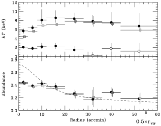
Figure 4: Radial variation of the temperature (top) and metal abundance (bottom) obtained from the annular spectral fits. The filled circles indicate results with the two-temperature model, the open circles are best-fit temperatures of the cool component whose significance are less than 99%. The open squares are for single-temperature fits in the energy range above 2 keV. The dashed line in the bottom panel shows an abundance profile when the metal mass density follows a $\beta$ model with $\beta=1.0$ and core radius of $11^{\prime}$, respectively.

These annular pulse-height spectra were then fitted with the 2-temperature model. As shown in table 3, the inclusion of the cool component gave a reduction of the $\chi^{2}$ value by 154.6, 98.7, 40.8, 32.2, 12.0 for a change of 2 degrees of freedom for the radii $0^{\prime}-4^{\prime},4^{\prime}-8^{\prime},8^{\prime}-12^{\prime},12^{\prime}-20^{\prime}$, and $20^{\prime}-28^{\prime}$, respectively, implying the cool emission to be significant at more than the 99% confidence (see Lampton et al. 1976). In figure 2(b), the fitting result for the annular region of $12^{\prime}<r<20^{\prime}$ is shown as an example,in which the residuals are for 2-temperature (middle panel) and single-tempelarature (bottom-panel) fits, respectively. In this series of spectral fits, we assumed common $N_{\rm H}$ and metal abundance for the two components based on the following reasons. The fits for the central-region spectrum showed that the common abundance is a reasonable assumption. Even though the free-$N_{\rm H}$ models for the cool component indicated 3 times higher absorption, the outer regions are likely to have only the Galactic $N_{\rm H}$. We also note that the lower statistics of the data in the outer regions hamper accurate determination of $N_{\rm H}$ and abundance for the cool component separately. The resultant spectral parameters and their 90% confidence limits are listed in table 3 and their radial variations are shown in figure 4 with filled circles. Results from single-temperature fits are also shows in table 3 and figure 4 for comparison.

One notable feature is that the hot spectral component shows a significant decline of temperature in the inner regions ($r<8^{\prime}$ or 250 kpc). The central “hot” temperature, 5.73 keV (less than 6.23 keV at the 90% confidence), is much lower than the outer values of about 8 keV at a radius of $10^{\prime}-30^{\prime}$. Since all the models fitted to the central spectrum in the previous section indicate the “hot” temperature to be less than 6.2 keV, it seems certain that the gas is cooling in the central region where the gas density is high. We need to note that the radial temperature profile in figure 4 is more extended than the true feature because of the point spread function. Ikebe et al. (1999) carried out the similar 2-temperature fit for the Centaurs cluster and found that the temperature of the hot component was constant with radius.

The cool spectral component with $kT\sim 2$ keV shows a large spatial extent and carries more than 20% of the total flux in the range $r=0^{\prime}-28^{\prime}$ and then drops to less than 10% in the outer regions, where the significance of the cool emission also becomes less than 90%. The fraction of the cool-component in the energy range 0.7 – 2 keV was obtained for each annular region and shown in table 3. By multiplying the cool component fraction to the PSPC flux in each annular region, the surface brightness profile of this component was calculated and shown in figure 5, which indicates that the emission is more extended than the point-spread function. The luminosity of the cool component is ($1.9\pm 0.5)\times 10^{44}$ erg s^-1 in 0.7–2 keV and ($3.7\pm 0.9)\times 10^{44}$ erg s^-1 in 0.1–10 keV, respectively, which is comparable to the total luminosity of fairly rich clusters.

As for the metal abundance, a slow decline as a function of radius is clearly seen in figure 4. The fit with the 2-temperature model indicates that the metal abundance is 0.44 (0.41–0.47) solar within $r=4^{\prime}$ and drops to 0.18 (0.10–0.27) solar at the outermost annular region of $r=44^{\prime}-60^{\prime}$, where $60^{\prime}$ corresponds to 1.8 Mpc at the source. Assumption of a constant abundance is rejected with $\chi^{2}=358.3$ for 7 DOF for the best-fit value of 0.255 solar. The abundances within $r=20^{\prime}$ are consistent with the BeppoSAX results (De Grandi and Molendi 2000). Since Fe-K emission line essentially determines the abundance parameter, this feature does not change much ($<10\%$) with the choice of 1 or 2 temperature models. The actual abundance profile must be steeper, but it is certainly broader than the point-spread function. Also, we note that the central abundance increase is not as strong as that in the Centaurs cluster (Fukazawa et al. 1994; Ikebe et al. 1999). As seen in the pulse-height spectra in figure 3, the relatively high temperature of the Perseus cluster makes the quantitative determination of the abundances of Si and other lighter elements difficult.

3.3 Azimuthal variation

To look into the spectral variation in different azimuthal directions, the data in the radial range $4^{\prime}-60^{\prime}$ were divided into north, west, south and east sectors and the resultant pulse-height spectra are shown in figure 6. Each sector covers an opening angle of $90^{\circ}$. The spectra show that the Fe-K line equivalent widths are different among the sectors, and the north and the east sectors show relatively strong iron lines. This feature strongly suggests that the metal abundance is significantly different along the azimuthal direction.

Based on the above spectral feature, we examined the radial variation of the hot-component spectrum for individual sectors. The ROSAT image was used again to obtain the “isothermal” response, and we fit the spectra with single temperature MEKAL models. Since the statistics of the data were much lower, 2-temperature models resulted in large uncertainties of the spectral parameters. Therefore, we have used the data only in the energy range above 2 keV and fit the data with single temperature models, which minimized the possible contamination from the cool component.

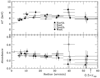
Figure 7: Radial variation of temperature and metal abundance in the 4 sectors.

For each sector, the obtained metal abundance and temperature are plotted as a function of radius in figure 7, with the parameter values shown in table 4. For comparison, the parameters for the sum of the 4 sectors are shown in table 4. We note in figure 4 that the single-temperature fit gives the consistent values to the 2-temperature fit, in the range $r>20^{\prime}$ for the temperature and in all radii for the abundance, respectively. In the azimuthally divided fit in $r=36^{\prime}-44^{\prime}$, the systematic errors of the temperature and metal abundance for a change of the background flux by 5% are 0.3 keV and 0.01 solar, respectively. Among the temperature profiles, the west sector shows a peak of about 8 keV in $r=12^{\prime}-20^{\prime}$, significantly higher than the other 3 data. In the outer regions, the north and the east sectors show a temperature jump at $r=36^{\prime}-44^{\prime}$. The significance for the temperature jump in the east is rather small, but at least the north point significantly deviates from the smooth declining trend of the temperature with radius. The detailed spatial variation of the temperature would be seen if a full 2-dimensional map of the ICM temperature is constructed, however this study requires extensive simulation of the ASCA mapping observation and is beyond the scope of the present paper.

As for the metal abundance, the sectors except for the east show a gradual decline with radius, similarly to the sum of all sectors. For each sector, constant abundance fits give $\chi^{2}$ values of 14.8, 6.95, 10.9, 19.2 with 6 DOF for north, east, south and west sectors respectively. Therefore, the abundance variation is significant at the 90 % confidence in 3 sectors excluding the east one. The east sector shows a significantly high value of 0.61 (0.42-0.82) solar at $r=36^{\prime}-44^{\prime}$, which is 2–3 times higher than the levels in other 3 sectors. The north sector, for example, shows a very low abundance of 0.11 (0-0.26) solar at this radius. This is the same radius where the high temperatures are seen in the north and the east. In other radii, 90% errors for all the sectors overlap. Therefore, only the east sector shows an unusual abundance behavior in this limited radial range. Note that these 4 sectors are symmetrically located around the cluster center, from which most of the flux contamination comes. Therefore, systematic differences in the response functions are small, and variation of the contaminating flux from the central $4^{\prime}$ region among the 4 sectors amounts to only 2% of the measured flux. This assures that the observed difference in the metal abundance is the real feature. To summarize the azimuthally divided analysis, both temperature and metal abundance show anomalous values in the same radial range ($36^{\prime}-44^{\prime}$) in the similar direction (north and east).

The gain parameters for the spectral fits shown in table 4 tend to be smaller than the unity, which was also pointed out by Dupke and Bregman (2001). However, the values are consistent to be the unity within the absolute gain accuracy of 1.2% except for the south sector at $r=4^{\prime}-8^{\prime}$ (0.977-0.985). As described in Makishima et al.(1996), the GIS gain varies largely with temperature by about 1% K^-1. Also, the temperature data from the satellite are quantized with a step of 0.55 K, which gives a gain error $\leq 0.5\%$. The long-term gain variation and the relationship between temperature and the gain are continuously monitored and shows a general scatter of 0.4%. Furthermore, the systematic uncertainty in the spatial variation of the gain in the GIS field is about 1% (see http://heasarc.gsfc.nasa.gov/docs/asca/cal_problem.html). By adding up these results, the GIS gain accuracy of 1.2–1.4% derived by Makishima et al. (1996) is considered as a very realistic estimate. We also looked into the GIS intrinsic spectral features at Au M-edge and Xe L-edge, however, the statistics was not enough to determine whether the Fe line shift was due to the gain variation or the redshift of the emission.

4 Discussion

The multi-pointing observations of the Perseus cluster from ASCA have shown significant variations in temperature and metal abundance over a large scale in the cluster. This is the first detection of such a large-scale variation in the spectral parameters in this cluster.

4.1 Spectral Softening in the Central Region

The energy spectra in the inner regions ($r<20^{\prime}$) are significantly softer than those in outer regions and require two temperature components. The cool component has a temperature $kT\sim 2$ keV, and the hot-component spectrum also shows a gradual softening with a temperature drop from 8 keV to 5.7 keV toward the center (see table 3 and figure 4). Fabian et al. (1994) showed that the SIS spectrum at the center of the Perseus cluster could be fitted either with a 2-temperature model ($kT=5.62$ keV and 2.05 keV) or with a cooling flow model, which is consistent with the present result.

The cool emission has a luminosity of $(3.7\pm 0.9)\times 10^{44}$ erg s^-1 estimated for an energy range 0.1–10 keV and integrated out to $r=28^{\prime}$. This is about 1/4 of the total X-ray luminosity of the cluster. This cool-to-total luminosity ratio is similar to the value obtained for the Centaurus cluster (Ikebe et al. 1999). The minimum mass of the cool component can be estimated by assuming a uniform region with the highest possible electron density (i.e. the central value). Taking $n_{e}=0.015$ after Ettori et al. (1998), the minimum mass of the cool component within a radius of $28^{\prime}$ becomes $\sim 3\times 10^{12}M_{\odot}$. This is much larger than the mass of the interstellar matter in the central cD galaxy. The observed luminosity and temperature of the cool component fall on the extension of the $L_{X}-kT$ relation derived for clusters of galaxies (see e.g. Mulchaey 2000), as if the cool component were a relaxed system with its own gravitational potential. This is probably not a coincidence since Ikebe et al. (2001) reported that the cool components in several clusters of galaxies he investigated also showed the consistent $L_{X}-kT$ relation with general clusters of galaxies.

Another significant feature in the central region is the softening of the hot-component spectrum toward the center within $r=8^{\prime}$. This trend is contrary to the Virgo cluster case, where the temperature of the hot component increases at the center (Shibata et al. 2000). At $r=8^{\prime}$, the electron density is $n_{e}\sim 3\times 10^{-3}$ cm^-3 (Ettori et al. 1998) and the cooling time due to the radiation becomes $t_{\rm cool}\sim 2.4\times 10^{10}$ yr. The radiation cooling could drop the temperature by 20% in a few Gyr, if there were no heat input through conduction from the surrounding region. Since the time scale for the thermal conduction in the central 250 kpc is only $10^{8}$ years (Spitzer 1956), suppression of the conductivity to less than 1% of the standard value would be necessary to maintain the temperature gradient (see also Ettori and Fabian 2000).

Recent XMM-Newton study of A1795 reveals that the temperature within $10^{\prime}$ ($\sim 1$ Mpc) from the center gradually drops from $kT=6.4$ keV to $2.2-2.4$ keV toward the center (Tamura et al. 2001). For this cluster, two-temperature fit for the ASCA spectrum within $3^{\prime}$ from the center showed $kT=6.54^{+0.56}_{-0.50}$ keV and $1.70^{+0.24}_{-0.26}$ keV (Xu et al. 1998), which approximately correspond to the maximum and the minimum temperatures in the observed field. Therefore, because of the insufficient angular resolution of ASCA XRT, the two-temperature feature in the GIS spectrum of the Perseus cluster is likely to indicate the range of temperature within the observed field which contains a strong temperature gradient.

4.2 Temperature Structure in the Outer region

In the outer region, the radial temperature profile in figure 4 shows a peak ($kT\sim 8.5$ keV) at around $15^{\prime}$ and then drops to $\sim 7$ keV in the outermost region. Markevitch et al. (1998) reported a universal temperature decrease with radius for 30 clusters, characterized by a factor of 2 drop at half the virial radius ($r_{\rm vir}$). For the Perseus cluster, $0.5r_{\rm vir}$ corresponds to 1.7 Mpc ($r=55^{\prime}$) and the observed temperature profile does not agree with a drop as much as factor of 2 at this radius. Recent results with ASCA (Kikuchi et al. 1999) and BeppoSAX (Irwin & Bregman 2000) for other clusters also indicate that the radial temperature profiles are more closer to being isothermal.

The non-radial temperature structures in the outer regions have been studied from Spartan (Snyder et al. 1990), ASCA (Arnaud et al. 1994), and ROSAT (Ettori et al. 1998), which all reported significant temperature variation. In particular, ROSAT PSPC observation indicated a cool emission with $kT\sim 3$ keV in the east between $20^{\prime}$ and $50^{\prime}$ from the center (Ettori et al. 1998). This region also showed an enhanced X-ray surface brightness with significant deviation from a smooth elliptical distribution, which suggested a subcluster merger (Schwarz et al. 1992). The ASCA temperatures in the four sectors indicate a fairly large scatter in the range $12^{\prime}-20^{\prime}$ and $36^{\prime}-44^{\prime}$ (see figure 7). In the inner region ($12^{\prime}-20^{\prime}$), the north sector is significantly hotter than other sectors. This may correspond to the hot region reported by Arnaud et al. (1994) based on the GIS data. However, these early ASCA results were not fully corrected for the energy dependent response of the X-ray telescope and may contain significant systematic errors. We also note that the reported cool region at $20^{\prime}-50^{\prime}$ in the east (Ettori et al. 1998) is not clearly recognized in the GIS data. Suppression of the data in the energy range below 2 keV in the analysis may have deprived our sensitivity to the cool emission. It is suggestive that, within $20^{\prime}-28^{\prime}$, the east sector indicates the lowest temperature.

The north and west sectors exhibit some hotter emission around $40^{\prime}$, which is close to the outer boundary of the residual emission when the smooth $\beta$-model is subtracted from the surface brightness data (Ettori et al. 1998). The metal abundance is high in the east and low in the north. The high metallicity suggests an enhanced star formation activity in the galaxies triggered by merger shocks, however with the present coarse resolution analysis the detailed feature seems to remain unresolved.

4.3 Metal Distribution

For the metal abundance, the GIS shows the central abundance within $4^{\prime}$ to be $0.44\pm 0.03$ solar. Our value is lower than the results from Spacelab 2 (0.7 solar for no point-source case, Ponman et al. 1990) and Spartan 1 (0.8 solar, Ulmer et al. 1987; Kowalski et al. 1993), but consistent with the Einstein SSS (0.44 solar, Mushotzky et al. 1981) and BBXRT ($\sim 0.5$ solar, Arnaud et al. 1992) results. Recent BeppoSAX observation also indicated 0.48 solar in the central $2^{\prime}$ region (Molendi et al. 1998). The present result is the first to show the metal abundance out to $1^{\circ}$ with enough sensitivity. The abundance profile shows a gradual decline except for a jump at about $40^{\prime}$ in the east and the outermost level is $0.18\pm 0.08$ solar. De Grandi and Molendi (2000) showed that the profile almost traces the optical light distribution of early type galaxies, but was slightly broader than the predicted ones. If the metals were to drift by about 50 kpc the profile can be explained.

It has been pointed out that the hot gas in the cluster center is opaque to a resonant scattering of Fe K$\alpha$ line (Gilfanov, Sunyaev, Churazov 1987), if there is no bulk motion of the gas. The scattering tends to smooth out the radial profile of the line intensity by conserving the total number of line photons. This effect was studied for the Perseus cluster with ASCA by Akimoto et al. (1999) and with BeppoSAX by Molendi et al. (1998). They predict that within $4^{\prime}$ from the center, the abundance estimated from Fe K$\alpha$ line is lower by a factor of about 2. If this is the case, as suggested from the Fe K$\beta$ line profile observed with BeppoSAX (Molendi et al. 1998), the central abundance should be about 0.9 solar which results in a strong gradient in the metal abundance. The dashed line in the bottom panel of figure 4 shows the expected abundance profile when the metal mass density follows a $\beta$ model with $\beta=1.0$ and core radius of $11^{\prime}$, respectively, which represents the distribution of cluster galaxies (Kent, Sargent 1983; Eyles et al. 1991). Therefore, in the Perseus cluster it is likely that the metal mass density traces the galaxy distribution, consistent with the feature previously observed in AWM 7 (Ezawa et al. 1997). To confirm the significance of the resonance scattering effect, observation of the cluster center with better energy resolution and angular resolution would be required (see also Böhringer et al. 2001).

Finally, the GIS spectra suggest a Fe-K line energy shift by about 1% in the south sector, similar to the feature reported by Dupke and Bregman (2001). However, the error range of the energy shift is smaller than the the absolute gain accuracy (1.2%) of the GIS, and we conclude there is no significant velocity gradient in the Perseus cluster.

The authors thank Dr. H. Böhringer and Dr. Y. Ikebe for useful discussion and the support in analyzing the ROSAT data. This work was partly supported by the Grants-in Aid for Scientific Research No. 08404010 and No. 12304009 from the Japan Society for the Promotion of Science.

References

Akimoto F., Furuzawa A., Tawara Y., Yamashita K. 1999, AN 320, 283 Allen S. W., Edge A. C., Fabian A. C., Böhringer H., Crawford C. S., Ebeling H., Johnstone R. M., Naylor T., Schwarz R. A. 1992, MNRAS 259, 67 Anders E., G‘revesse N. 1989, Geochemica et Cosmochemica Acta 53, 197 Arnaud K. A., Mushotzky R. F., Serlemitsos P. J., Boldt E., Holt S. S., Jahoda K., Marshall F. E., Petre R. et al. 1992 in Proc. Ginga Memorial Symp., ed. F. Makino & F. Nagase (Tokyo: ISAS) 114 Arnaud K. A., Mushotzky R. F., Ezawa H., Fukazawa Y., Ohashi T., Bautz M. W., Crewe G. B., Gendreau K. C. et al. 1994, ApJ 436, L67 W., Fabian A.C., Edge A.C., Neumann D.M. 1993, MNRAS, 264, L25 Böhringer, H., Belsole, E., Kennea, J., Matsushita, K., Molendi, S., Worrall, D. M., Mushotzky, R. F., Ehle, M., et al. 2001, A&A, 356, L181 Churazov E., Gilfanov M., Forman W., Jones C. 1999, ApJ 520, 105 Churazov E.,Forman W., Jones C., Böhringer H. 2000, A&A 356, 788 De Grandi S., Molendi S. 2000, ApJ accepted astro-ph/0012232 Dupke R., Arnaud K. 1999, AN 320, 284 Dupke R.A., Bregman J.N. 2001, ApJ 547, 705 Ettori S., Fabian A. C., White D. A. 1998, MNRAS 300, 837 Eyles C. J., Watt M. P., Bertram D., Church M. J., Ponman T. J., Skinner G. K., Willmore A. P. 1991, ApJ 376, 23 Ezawa H., Fukazawa Y., Makishima K., Ohashi T., Takahara F., Xu H., Yamasaki N. Y. 1997, ApJ 490, L33 Fabian A. C., Arnaud K. A., Bautz M. W., Tawara Y. 1994, ApJ 436, L63 Fabian A.C., Sanders J.S., Ettori S., Taylor G.B., Allen S.W., Crawford C.S., Iwasawa K., Johnstone R.M., Ogle P.M. 2000, MNRAS 318, L65 Fukazawa Y., Ohashi T., Fabian A. C., Canizares C. R., Ikebe Y., Makishima K., Mushotzky R. F., Yamashita K. 1994, PASJ 44, L55 Furusho T., Yamasaki N.Y., Ohashi T., Shibata R., Kagei T., Ishisaki Y., Kikuchi K., Ezawa H., Ikebe Y. 2000, PASJ accepted Gilfanov M. R., Sunyaev R. A., Churazov E. M. 1987, Soviet Astronomy Letters 13, 3 Honda H., Hirayama M., Watanabe M., Kunieda H., Tawara Y., Yamashita K., Ohashi T., Hughes J. P., Henry J. P. 1996, ApJ 473, L71 Ikebe Y., Ph.D thesis, 1995, University of Tokyo Ikebe Y., Makishima K., Ezawa H., Fukazawa Y., Hirayama M., Honda H., Ishisaki Y., Kikuchi K. et al. 1997, ApJ 481, 660 Ikebe Y., Makishima K., Fukazawa Y., Tamura T., Xu H., Ohashi T., Matsushita K. 1999, ApJ 525, 58 Böhringer, H., & Tanaka, Y., presentaion at “New Century of X-ray Astronomy”, Yokohama, March, 2001
or private communication ? Ishisaki Y., Ueda Y., Kubo H., Ikebe Y., Makishima K. and the GIS team 1997 ASCA News No 5, 26 Irwin J.A., Bregman J.N. 2000, ApJ 538, 543 Kent S. M., Sargent W. L. W. 1983, AJ 88, 697 Kikuchi K., Furusho T., Ezawa H., Yamasaki N. Y., Ohashi T., Fukazawa Y., Ikebe Y. 1999, PASJ 51, 301 Kowalski M. P., Cruddace R. G., Snyder W. A., Frits G. G., Ulmer M. P., Fenimore E. E. 1993, ApJ 412, 489 Lampton M., Margon B., Bowyer S. 1976, ApJ Letter 208, 177 Makishima K., Tashiro M., Ebisawa K., Ezawa H., Fukazawa Y., Gunji S., Hirayama M., Idesawa E. et al. 1996, PASJ 48, 171 Markevitch M., Forman W. R.; Sarazin C. L., Vikhlinin A. 1998, ApJ 503, 77 Molendi S., Matt G., Antonelli L. A., Fiore F., Fusco-Femiano R., Kaastra J., Maccarone C., Perola C. 1998, ApJ 499, 608 Mushotzky R. F., Holt S. S., Smith B. W., Boldt E. A., Serlemitsos P. J. 1981, ApJ 244, L47 Ohashi T., Ebisawa K., Fukazawa Y., Hiyoshi K., Horii M., Ikebe Y., Ikeda H., Inoue H. Ishida M. 1996, PASJ 48, 157 Peterson J.R., Paerels F.B.S., Kaastra J.S., Arnaud M., Reiprich T.H., Fabian A.C., Mushotzky R.F., Jernigan J.G., Sakelliou I. 2000, A&A Letters 365, 104 Ponman T. J., Bertram D., Church M. J., Eyles C. J., Watt M. P., Skinner G. K., Willmore A. P. 1990, Nature 347, 450 Mulchaey J.S. 2000 Ann. Rev. Astron. Astrophys., 38, 289 Schwarz R. A., Edge A. C., Voges W., Böhringer H., Ebeling H., Briel U. G. 1992, A&A 256, L11 Shibata R., Matsusita K., Yamasaki N.Y., Ohashi T., Ishida M., Kikuchi K., Böhringer H., Matsumoto H. 2001, ApJ 549, 228 Snyder W. A., Kowalski M. P., Cruddace R. G., Fritz G. G., Middleditch J., Fenimore E. E., Ulmer M. P., Majewski S. R. 1990, ApJ 365, 460 Spitzer, L. 1956, Physics of Fully Ionized Gases, Interscience Publishers, New York Takahashi T., Markevitch M., Fukazawa Y., Ikebe Y., Ishisaki Y., Kikuchi K., Makishima K., Tawara Y. et al. 1995, ASCA News 3, 24 Tamura T., Kaastra J.S., Peterson J.R., Paerels F., Mittaz P.D., Trudolyubiv S.P., Stewart G., Fabian A.C. et al. 2001 A&A Letters 365, 87 Tanaka Y., Inoue H., Holt S. S. 1994, PASJ 46, L37 Ulmer M. P., Cruddace R. G., Fritz G. G., Snyder W. A., Fenimore E. E. 1987, ApJ 319, 118 Watanabe M., Yamashita K., Furuzawa A., Kunieda H., Tawara, Y., Honda, H. 1999, ApJ 527, 80 Xu H., Makishima K., Fukazawa Y., Ikebe Y., Kikuchi K., Ohashi T., Tamura T. 1998, ApJ 500, 538

Figure 1: The X-ray image of the Perseus cluster observed with the ASCA GIS. Each pointed field is shown with a circle of $40^{\prime}$ diameter, representing the GIS field of view. The energy range is 0.7–10 keV.

(a)

(b)

Figure 2: Pulse-height spectra for the central region ($r<4^{\prime}$) (a) and the annular region ($12^{\prime}<r<20^{\prime}$) (b) of the Perseus cluster for the sum of the GIS2 and GIS3 data. The 2-temperature model with fixed $N_{\rm H}$ and common abundance (the first row in table 2) are fitted to the data, and the middle panels shows the residual of the fit. The bottom panels shows the residuals when the data are fitted by 1-temperature model with the same $N_{\rm H}$.

Figure 3: Energy spectra obtained by the GIS for 4 concentric annular regions in the Perseus cluster. The gradual decrease of the Fe K-line equivalent width as a function of radius is suggested.

Figure 5: Surface brightness distribution of the cool component, compared with the PSPC radial profile and the point spread function of the GIS instrument. The emission is extended.

Figure 6: Pulse-height spectra for the four $90^{\circ}$ sectors in the radius range $28^{\prime}-60^{\prime}$. The Fe line equivalent widths are different among the sectors.

Table 1: Summary of ASCA observations

Sequential	Observation	Exposure	FOV center
No.	Start (UT)	(sec.)	$\alpha_{2000}$	$\delta_{2000}$
80007000	93/08/06 04:19	11737	50.040	41.619
80008000	93/08/06 18:30	18449	49.630	41.537
80009000	93/09/15 00:39	16978	49.264	41.546
81026000	94/02/09 17:13	19862	49.284	41.407
81027000	94/02/10 03:10	16935	48.888	41.258
83051000	95/08/18 20:06	10307	50.325	41.538
83052000	95/08/19 12:11	15817	50.677	41.537
83053000	95/09/04 13:06	13330	50.057	41.287
85000000	97/02/14 11:22	18233	50.516	41.961
85001000	97/02/14 23:51	18108	49.895	42.103
85002000	97/02/15 12:42	15501	49.423	41.923
85003000	97/02/16 19:50	17974	50.449	41.023
85004000	97/02/17 09:11	18490	49.721	40.930

Table 2: Spectral fits for the central region within the radius of $4^{\prime}$.

$N_{\rm Hhot}$	$kT_{\rm hot}$	$Z_{\rm hot}$	$N_{\rm Hcool}$	$kT_{\rm cool}$	$Z_{\rm cool}$	$\chi^{2}$/dof
(1021cm-2)	(keV)		(1021cm-2)	(keV)
1.4(fix)	5.73(5.15-6.23)	0.442(0.413-0.470)	$=N_{\rm Hhot}$	2.05(1.76-2.26)	$=Z_{\rm hot}$	149.8/121
1.4(fix)	5.66(5.21-6.22)	0.458(0.422-0.503)	$=N_{\rm Hhot}$	1.91(1.71-2.21)	0.342(0.250-0.664)	148.0/120
1.63(1.42-1.84)	5.43(5.08-6.04)	0.432(0.422-0.503)	$=N_{\rm Hhot}$	1.75(1.56-2.14)	$=Z_{\rm hot}$	146.7/120
2.03(1.62-2.32)	5.32(5.06-5.57)	0.449(0.422-0.477)	$=N_{\rm Hhot}$	1.37(1.27-1.73)	0.223(0.170-0.291)	138.8/119
1.4(fix)	5.27(5.04-5.52)	0.440(0.416-0.465)	4.92(3.58-6.28)	1.30(1.17-1.40)	$=Z_{\rm hot}$	132.7/120
1.4(fix)	5.23(4.97-5.50)	0.436(0.409-0.463)	4.92(3.58-6.28)	1.29(1.16-1.40)	0.548(0.328-1.14)	132.3/119

Note: $Z$ represents metal abundance, and the values in parenthesis indicate single-parameter 90% limits.

Table 3: Spectral fits for the annular regions

radius	$kT_{\rm hot}$ (keV)	$Z$	$kT_{\rm cool}$ (keV)	Cool fraction (%)	gain	$\chi^{2}$/dof
0-4	5.73(5.15-6.23)	0.442(0.413-0.470)	2.05(1.76-2.26)	34.2(22.6-44.7)	0.996(0.993-0.998)	149.96/121
	4.09(4.05-4.12)	0.496(0.474-0.519)	–	–	0.994(0.993-0.994)	304.52/123
4-8	6.37(5.97-6.95)	0.387(0.361-0.416)	1.77(1.53-2.15)	18.5(12.8-28.8)	0.999(0.995-1.0)	137.08/121
	5.21(5.15-5.28)	0.411(0.388-0.434)	–	–	0.994(0.993-0.995)	235.78/123
8-12	8.06(7.25-10.4)	0.422(0.377-0.480)	2.16(1.63-3.0)	17.8(9.2-38.6)	0.993(0.990-0.993)	111.54/121
	6.42(6.30-6.55)	0.411(0.380-0.442)	–	–	0.990(0.988-0.992)	152.35/123
12-20	8.57(7.55-10.2)	0.378(0.333-0.431)	2.31(1.64-3.0)	18.2(7.9-35.3)	0.993(0.990-0.994)	117.29/121
	6.79(6.66-6.91)	0.357(0.328-0.386)	–	–	0.990(0.989-0.992)	149.46/123
20-28	8.39(7.53-9.68)	0.265(0.208-0.323)	1.44(0.95-2.24)	8.5(3.4-26.4)	0.993(0.989-1.0)	111.98/121
	7.34(7.11-7.60)	0.277(0.225-0.330)	–	–	0.989(0.989-0.994)	123.93/123
28-36	7.81(7.05-9.20)	0.173(0.087-0.323)	0.22(0.09-0.95)	6.7(0.0-30.2)	0.998(0.978-1.01)	85.97/121
	7.94(7.20-8.86)	0.208(0.054-0.364)	–	–	0.986(0.973-0.997)	87.87/123
36-44	7.54(6.95-9.82)	0.287(0.224-0.361)	1.76(0-3.0)	4.0(0.0-27.7)	0.983(0.978-0.991)	108.00/121
	7.14(6.88-7.40)	0.291(0.231-0.352)	–	–	0.983(0.979-0.987)	109.12/123
44-60	6.73(5.70-9.59)	0.183(0.100-0.266)	1.16(0.50-3.0)	5.6(0.0-56.0)	0.988(0.980-1.0)	76.50/121
	5.89(5.64-6.24)	0.200(0.122-0.280)	–	–	0.983(0.980-0.991)	79.39/123

Note: 0.7-9 keV, $N_{\rm H}$ is fixed to the Galactic value $1.4\times 10^{21}$ cm^-2. One and two-component MEKAL model is used. Cool fraction is the ratio of the cool-component to the total fluxes in the energy range 0.7 – 2 keV.

Table 4: Spectral fits for the four sectors

radius(arcmin)	$kT$ (keV)	$Z$	gain	$\chi^{2}$/dof
All sectors
0-4	4.36(4.29-4.43)	0.427(0.402-0.451)	0.9996(0.9988-0.9997)	129.68/70
4-8	5.60(5.49-5.72)	0.372(0.348-0.397)	0.999(0.998-1.0)	104.88/70
8-12	6.82(6.61-7.03)	0.384(0.352-0.417)	0.998(0.995-1.0)	76.72/70
12-20	7.07(6.86-7.28)	0.343(0.313-0.374)	0.998(0.993-0.999)	82.62/70
20-28	7.82(7.36-8.36)	0.246(0.190-0.301)	0.999(0.990-1.004)	53.81/70
28-36	7.58(6.56-9.07)	0.209(0.055-0.364)	0.986(0.967-1.011)	43.40/70
36-44	7.23(6.79-7.72)	0.279(0.216-0.341)	0.988(0.978-0.994)	79.26/70
44-60	5.85(5.40-6.45)	0.190(0.106-0.276)	0.989(0.976-1.0)	43.82/70
North
4-8	5.21 (4.95-5.48)	0.323(0.267-0.381)	1.000(0.995-1.007)	69.70/70
8-12	5.94 (5.57-6.44)	0.379(0.304-0.459)	0.999(0.991-1.002)	81.35/70
12-20	6.23 (5.76-6.74)	0.314(0.240-0.389)	0.990(0.989-1.001)	67.98/70
20-28	6.89 (6.41-7.39)	0.322(0.243-0.383)	1.000(0.990-1.008)	72.11/70
28-36	6.18 (5.75-6.72)	0.326(0.228-0.406)	1.001(0.990-1.007)	82.85/70
36-44	9.09 (7.50-10.96)	0.107(0.0 -0.256)	0.989(0.964-1.007)	71.83/70
44-60	6.47 (5.25-8.24)	0.090(0.0 -0.311)	1.001(0.965-1.029)	98.48/70
East
4-8	5.83(5.58-6.13)	0.321(0.271-0.371)	0.998(0.991-1.000)	73.17/70
8-12	6.40(6.04-6.78)	0.321(0.265-0.377)	1.009(1.000-1.011)	69.46/70
12-20	6.27(5.96-6.58)	0.339(0.293-0.386)	0.999(0.994-1.004)	77.40/70
20-28	5.73(5.45-6.05)	0.316(0.260-0.374)	0.996(0.989-1.001)	61.78/70
28-36	6.72(6.16-7.31)	0.369(0.283-0.455)	0.989(0.980-0.998)	68.61/70
36-44	8.14(6.96-9.67)	0.609(0.419-0.815)	0.984(0.972-1.000)	63.73/70
44-60	5.87(4.78-7.54)	0.225(0.0-0.456)	0.941(0.930-1.031)	57.02/70
South
4-8	5.72(5.42-6.04)	0.416(0.350-0.484)	1.000(0.998-1.005)	84.04/70
8-12	7.65(7.10-8.35)	0.361(0.285-0.437)	0.985(0.977-0.988)	69.40/70
12-20	6.93(6.45-7.42)	0.373(0.300-0.445)	1.000(0.990-1.005)	71.91/70
20-28	6.43(6.04-6.83)	0.285(0.229-0.342)	0.998(0.989-1.003)	83.05/70
28-36	6.69(6.15-7.26)	0.367(0.282-0.452)	0.997(0.984-1.000)	55.50/70
36-44	6.86(5.97-7.91)	0.301(0.168-0.437)	0.967(0.955-0.989)	72.30/70
44-60	5.05(4.18-6.21)	0.138(0.0 -0.350)	0.970(0.929-1.000)	67.03/70
West
4-8	5.44(5.24-5.65)	0.373(0.328-0.419)	1.000(0.995-1.000)	84.69/70
8-12	7.32(6.91-7.83)	0.435(0.371-0.501)	0.988(0.985-1.000)	89.10/70
12-20	8.15(7.58-8.75)	0.308(0.246-0.371)	0.999(0.996-1.002)	91.14/70
20-28	7.33(6.99-7.73)	0.294(0.245-0.344)	0.999(0.995-1.007)	76.85/70
28-36	6.92(6.44-7.41)	0.264(0.197-0.333)	0.993(0.989-1.004)	57.96/70
36-44	6.15(5.67-6.76)	0.214(0.131-0.298)	0.997(0.982-1.007)	56.78/70
44-60	5.62(5.04-6.35)	0.310(0.189-0.436)	0.986(0.972-0.999)	49.79/70

Note: 2-9keV 1 component,$N_{\rm H}$ is fixed to the Galactic value $1.4\times 10^{21}$ cm^-2.