Microlensing and the Surface Brightness Profile
of the Afterglow Image of GRB 000301C

Abstract

The optical afterglow of Gamma-Ray Burst (GRB) 000301C exhibited a significant, short-timescale deviation from the power-law flux decline expected in the standard synchrotron shock model. Garnavich, Loeb & Stanek found that this deviation was well-fit by an ad hoc model in which a thin ring of emission is microlensed by an intervening star. We revisit the microlensing interpretation of this variability, first by testing whether microlensing of afterglow images with realistic surface brightness profiles (SBPs) can fit the data, and second by directly inverting the observed light curve to obtain a non-parametric measurement of the SBP. We find that microlensing of realistic SBPs can reproduce the observed deviation, provided that the optical emission arises from frequencies above the cooling break. Conversely, if the variability is indeed caused by microlensing, the SBP must be significantly limb-brightened. Specifically, $\geq 60\%$ of the flux must originate from the outer $25\%$ of the area of the afterglow image. The latter requirement is satisfied by the best fit theoretical SBP. The underlying optical/infrared afterglow lightcurve is consistent with a model in which a jet is propagating into a uniform medium with the cooling break frequency below the optical band.

gamma rays:bursts – gravitational lensing

1 Introduction

The afterglows of gamma-ray bursts (GRBs) are observed in the X-ray, optical, near-infrared, and radio, and appear to be well-described by the synchrotron blast-wave model in which the source ejects material with a relativistic bulk Lorentz factor, driving a relativistic shock into the external medium (see Van Paradijs et al. 2000; Piran 2000 and references therein). There is mounting evidence from the observed steepening of afterglow light curves that these ejecta are in many cases mildly to highly collimated, with opening angles $\sim 3$–$30^{\circ}$ (Harrison et al., 1999; Frail et al., 2000, 2001). Global fitting of the afterglow light curves over many decades in time and frequency, in the context of this model, can be used to derive constraints on the physical parameters of the model, i.e., the energy and opening angle of the jet, the external density, the magnetic field strength and the energy distribution of the electrons behind the shock (Wijers & Galama, 1999; Freedman & Waxman, 2001; Panaitescu & Kumar, 2001).

In this model, the image of the afterglow is expected to appear highly limb brightened at frequencies above the peak synchrotron frequency $\nu_{\rm m}$, but more uniform at frequencies $<\nu_{\rm m}$, especially below the self–absorption frequency $\nu_{a}$ (Waxman 1997; Sari 1998; Panaitescu & Mészáros 1998; Granot, Piran, & Sari 1999a,b; Granot & Loeb 2001). A measurement of the surface brightness profile (SBP) at several frequencies would thus provide an important test of the model. For typical parameters, the afterglow image expands superluminally, and has an angular radius ${\cal O}(\mu{\rm as})$ a few days after the GRB. As pointed out by Loeb & Perna (1998), this is of the same order as the angular Einstein ring radius of a solar mass lens at cosmological distances,

$$\theta_{\rm E}=\left({4GM\over c^{2}D}\right)^{1/2}=1.6\left({M\over M_{\odot}}\right)^{1/2}\left({D\over 10^{28}~{}{\rm cm}}\right)^{-1/2}\mu{\rm as},$$ (1)

where $M$ is the lens mass, and $D\equiv D_{os}D_{ol}/D_{ls}$, and $D_{os}$, $D_{ol}$ and $D_{ls}$ are the angular diameter distances between the observer-source, observer-lens, and lens-source, respectively. Thus lensing by a star along the line of sight will produce a detectable magnification over the course of a few days to weeks. The probability that any given GRB will be microlensed is $\sim 1\%b^{2}$, where $b$ is the angular separation between the GRB and lens in units of $\theta_{\rm E}$. Since the original suggestion by Loeb & Perna (1998), this application of microlensing has been studied by several authors (Mao & Loeb, 2001; Koopmans & Wambsganss, 2001; Granot & Loeb, 2001; Gaudi & Loeb, 2001; Ioka & Nakamura, 2001).

The well-sampled optical afterglow of GRB 000301C exhibited a short time scale, nearly achromatic deviation from the nominal power-law flux decline. Garnavich, Loeb & Stanek (2000; hereafter GLS) found that this deviation is well-fit by a model in which the afterglow was microlensed by an intervening star. However, the model they adopted for the SBP was somewhat crude: they assumed the emission arose solely from an outer ring of fractional width $W$, with $W\simeq 10\%$ providing the best fit to the data. Recently, Panaitescu (2001) argued that, if one adopts realistic SBPs, microlensing cannot explain the data. Here we revisit the microlensing interpretation of this deviation. We fit the optical/infrared dataset of GRB 000301C to a double-power law plus microlensing model, adopting realistic SBPs, and, under the assumption that the observed deviation is indeed due to microlensing, we directly invert the light curve, obtaining a non-parametric measurement of the SBP, and compare this measurement to theoretical expectations.

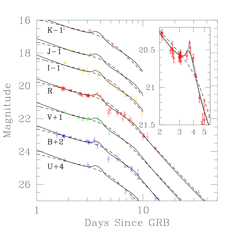
Figure 1: $UBVRIJK$ photometry of GRB 000301C as a function of days from the GRB. Points have been offset by the indicated amount for clarity. The dashed line is the best-fit double power law (with no lensing), while the solid line is the overall best-fit microlensing model, where the SBP has been determined from direct inversion. The inset shows the $R$-band data only. The dotted line is the best-fit microlensing model with theoretically calculated SBP, in this case for $k=0$ and $\nu>\nu_{c}$.

2 Data

We will be considering the same dataset as GLS, namely 104 photometric data points in the $UBVRIJK$-bands distributed as $(6,18,8,46,16,3,7)$. These data, shown in Figure 1, are taken from the compilation of Sagar et al. (2000) with additional photometry from Stanek et al. (2000). We will not consider the data in the radio regime (Berger et al., 2000), as the majority is not contemporaneous with the optical deviation. For more details on the GRB itself and the optical, infrared and radio data, see GLS, Masetti et al. (2000), Sagar et al. (2000), Berger et al. (2000) and Rhoads & Fruchter (2000).

3 Theoretical Surface Brightness Profiles

The magnitude, shape, and duration of the microlensing signal depends sensitively on the SBP of the afterglow (Loeb & Perna, 1998; Mao & Loeb, 2001; Granot & Loeb, 2001). The SBP, in turn, depends on the observed frequency and the physical parameters of the shock. Thus detailed measurements of a microlensed afterglow light curve can be used to constrain the physical parameters of the afterglow. However, the expected SBPs in the relativistic blast-wave model can also be calculated a priori under various assumptions (Waxman, 1997; Sari, 1998; Granot, Piran & Sari, 1999a, b; Granot & Loeb, 2001; Ioka & Nakamura, 2001; Panaitescu, 2001). Thus one can alternatively use the theoretical SBPs to calculate the expected microlensing signature, thereby confirming or refuting the microlensing interpretation. This was the approach taken by Panaitescu (2001). We adopt both approaches here.

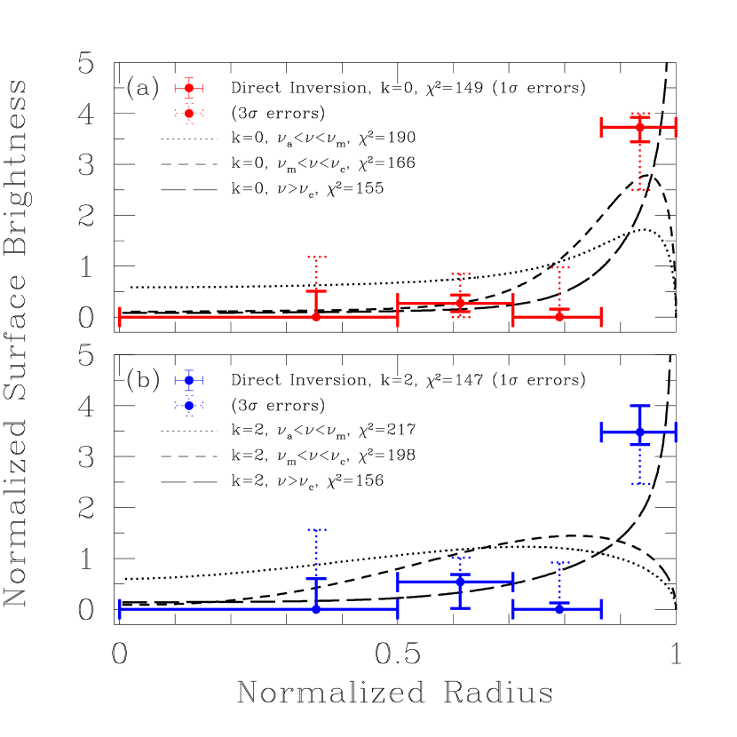
Figure 2: SBPs as a function of normalized radius. The points are the SBPs determined from direct inversion, with $1\sigma$ errors (solid) and $3\sigma$ errors (dotted). The curves are theoretically calculated SBPs for various frequency regimes (see Granot & Loeb 2001). (a) Uniform external medium, $k=0$. (b) Stellar wind environment, $k=2$.

We calculate SBPs using the method described in Granot & Sari (2001) and Granot & Loeb (2001). Briefly, the hydrodynamics are described by the Blandford-McKee (1976; BM hereafter) self-similar solution, assuming a power-law external density profile, $\rho(r)\propto r^{-k}$, and a power-law number versus energy distribution of electrons with index $p$, ${\rm d}N_{e}/{\rm d}\gamma\propto\gamma^{-p}$, just behind the shock, which thereafter evolves due to radiative and adiabatic losses. We integrate the emission over the entire volume behind the shock front. A few days after the burst the afterglow is typically in the slow cooling regime (i.e. a typical electron cools on a timescale larger than the dynamical time) and the ordering of the break frequencies is $\nu_{a}<\nu_{m}<\nu_{c}$, where $\nu_{c}$ is the cooling frequency (Sari, Piran, & Narayan, 1998; Granot, Piran & Sari, 1999a; Chevalier & Li, 2000). We assume that this is the case for GRB 000301C, as indicated by Berger et al. (2000). We consider only the SBPs from frequencies $\nu>\nu_{a}$, since after a few days the optical band is typically well above $\nu_{a}$ (and usually also above $\nu_{m}$). The spectrum consists of several power-law segments (PLSs), where $F_{\nu}\propto\nu^{\beta}t^{\alpha}$ (see Figure 1 in Granot & Loeb 2001). Due to the self-similar nature of the hydrodynamics, the normalized SBP within a given PLS is independent of time (though it changes considerably between different PLSs). Thus, for each $k$, there are 3 relevant forms for the SBP, each corresponding to a different PLS: $\beta=1/3$ ($\nu_{a}<\nu<\nu_{m}$), $\beta=(1-p)/2$ ($\nu_{m}<\nu<\nu_{c}$) and $\beta=-p/2$ ($\nu>\nu_{c}$). The corresponding values of the temporal index $\alpha$ for $k=0$ ($k=2$) are $\alpha=1/2$ ($\alpha=0$) for $\beta=1/3$, $\alpha=-3(p-1)/4$ ($\alpha=-(3p-1)/4$) for $\beta=(1-p)/2$ and $\alpha=-(3p-2)/4$ (for both $k=0$ and $k=2$) for $\beta=-p/2$.

The expected SBPs are shown in Figure 2, for a uniform external medium $k=0$, and a stellar wind environment $k=2$. Note that the SBP becomes more limb-brightened as the frequency goes to a higher PLS, i.e. the spectral slope $\beta$ is reduced, or as the value of $k$ is reduced.

4 Analysis and Model Fitting

We fit the data of the flux as a function of time to the form of two asymptotic power-laws which join smoothly:

$$F_{\nu}(t)=\mu(t)F_{0,\nu}\left[\left({t\over t_{\rm b}}\right)^{-s\alpha_{1}}+\left({t\over t_{\rm b}}\right)^{-s\alpha_{2}}\right]^{-1/s},$$ (2)

where $t_{\rm b}$ is the “break time,” $F_{0,\nu}$ is the unlensed flux at the point where the asymptotic power laws before and after the break meet, $\alpha_{1}$ and $\alpha_{2}$ are the indices of the flux decline, and $s$ is a sharpness parameter; the larger the value of $s$, the sharper the break. The magnification $\mu$ due to microlensing depends on the impact parameter $b$, the radial SBP of the afterglow image, and the angular size of the afterglow in units of $\theta_{\rm E}$,

$$R_{\rm s}={R_{0}{t_{\rm day}}^{\delta}}.~{}$$ (3)

Here $\delta=(5-k)/2(4-k)$, ${t_{\rm day}}$ is the time from the GRB in days and $R_{0}$ is the value of $R_{s}$ after 1 day. The light curve exhibits an achromatic break at $t_{\rm b}\sim 7$ days. Berger et al. (2000) find that this break can be well explained by jet with $k=0$, while Panaitescu (2001) argues that a jet alone cannot produce the required steepening of the light curve, and invokes a double power law electron distribution, which causes additional (though chromatic) steepening of the light curve if the synchrotron frequency corresponding to the break in the electron distribution crosses the optical band around $t_{\rm b}$. Either way, we would expect the SBP at $t{{}_{>}\atop{}^{{}^{\sim}}}t_{\rm b}$ to be different than at $t{{}_{<}\atop{}^{{}^{\sim}}}t_{\rm b}$. However, our best fit models give $t_{\rm b}\sim 8~{}$days, while the majority of the constraints on the SBP come from times $t{{}_{<}\atop{}^{{}^{\sim}}}8~{}$days, where the spherical self-similar BM solution should still be applicable, resulting in the self-similar SBPs described in §3. We will therefore adopt the simpler (and self consistent) working assumption that the SBP, when normalized to its average value, as a function of radius normalized to $R_{\rm s}$, is independent of time within a given PLS.

The model in equation (2) is a function of $N_{\rm par}=4+N_{l}+2$ free parameters: four parameters describe the shape of the broken power-law ($\alpha_{1},\alpha_{2},s,t_{\rm b}$); one parameter provides the normalization $F_{0,\nu}$ for each of $N_{l}$ frequency bands and two additional parameters describe the microlensing effect ($b,R_{0}$) for a given SBP. Considering all the data for GRB 000301C in Figure 1, there are $11$ parameters without microlensing, and $13$ free parameters with microlensing using theoretically-calculated SBPs. For comparison purposes, we also fit the data to the model adopted by GLS: we assume that the source emission is confined to a thin ring of fractional width $W$. However, we extend the model of GLS by allowing the image interior to the ring to have a relative surface brightness $C$ referenced to the outer ring ($C=0$ reduces to the GLS model). This model introduces two additional free parameters. Finally, we consider a non-parametric fit (“direct inversion”) to the SBP. We divide the image into $N_{\rm bin}$ equal-area annuli, and find the fraction $f_{i}$ of the total flux contributed by each bin $i$. In this case the magnification is given by $\mu=\sum_{i}f_{i}\mu_{i}$, where $\mu_{i}$ is the magnification of annulus $i$. This adds an additional $N_{\rm bin}-1$ parameters (due to the constraint that $\sum_{i}f_{i}=1$). We find the best-fit solution by minimizing $\chi^{2}$ with respect to all of these parameters. We define the $1\sigma$ errors on these parameters as the projection of the $\Delta\chi^{2}=1$ hypersurface on the parameter axes, where

$$\Delta\chi^{2}\equiv{{\chi^{2}-\chi^{2}_{\rm min}}\over\chi^{2}_{\rm min}/{\rm dof}},$$ (4)

$\chi^{2}_{\rm min}$ is the minimum $\chi^{2}$ for a given model, and ${\rm dof}=104-N_{\rm par}$ is the number of degrees of freedom for the 104 data points. We normalize $\Delta\chi^{2}$ by the factor $\chi^{2}_{\rm min}/{\rm dof}$ because we believe that the errors on the data points are likely underestimated, resulting in inflated values of $\chi^{2}$. Errors on the fit parameters determined using these inflated values of $\chi^{2}$ would be significantly underestimated.

5 Results

Figure 1 shows the best fit for the double power-law model with no lensing. The best-fit parameters and $1\sigma$ errors for $(\alpha_{1},\alpha_{2},s,t_{\rm b})$ are tabulated in Table 1. The fit is poor: $\chi^{2}=240.7$ for $93$ dof. Residuals from the broken power-law model are shown in Figure 3; the systematic deviations from this model are apparent.

When microlensing is included, the fit improves considerably. For the extended GLS model, we find that the data is best explained by emission solely from an outer ring of relatively small fractional width. Specifically, we find best-fit parameters, $W=0.13^{+0.04}_{-0.07}$, $C=0^{+0.02}$ for $k=0$ and $W=0.16_{-0.08}^{+0.03}$, $C=0^{+0.03}$ for $k=2$. The remaining parameters and the best-fit $\chi^{2}$ are shown in Table 1. The parameters we find differ from those of GLS, and we find a $\chi^{2}/{\rm dof}$ smaller than they report. However, when we evaluate their model fit, we recover their $\chi^{2}/{\rm dof}$, indicating that their fit was likely a local, not global, minimum. For the fits with microlensing, we find that the sharpness parameter $s$ is not well constrained, but is always $s{{}_{>}\atop{}^{{}^{\sim}}}5$, indicating a sharp break. To avoid excessive covariances with other parameters, we fix $s=20$ for the remaining fits, thus reducing $N_{\rm par}$ by one. The results are essentially identical for other values of $s{{}_{>}\atop{}^{{}^{\sim}}}5$. For a uniform external medium ($k=0$), for which one generally predicts more limb-brightened SBPs, we find $\chi^{2}=190.0,166.1$, and $154.7$ for $\nu_{a}<\nu<\nu_{m}$, $\nu_{m}<\nu<\nu_{c}$, and $\nu>\nu_{c}$, respectively. For the case of a wind-like medium ($k=2$), the fits are generally worse: $\chi^{2}=216.8,197.9$, and $155.5$ for the same frequency ranges. The deviations of these fits from the double power-law model are shown in Figure 3. It is clear that a significantly limb-brightened profile is required to fit the sharp, large deviation at $t\sim 4$ days. For $\nu>\nu_{c}$, both wind and uniform external media provide satisfactory fits to the data. For $\nu_{m}<\nu<\nu_{c}$, the uniform medium provides a marginal fit. Frequencies below the peak synchrotron frequency $\nu_{m}$, or $\nu_{m}<\nu<\nu_{c}$ with a wind-like medium ($k=2$), result in SBPs that are too uniform to fit the data.

For the non-parametric SBP fit to the data, we impose the condition that $f_{i}\geq 0$, and we increase the number of bins $N_{\rm bin}$ in the recovered SBP until $\chi^{2}$ changes by $\leq 1$. We find that $N_{\rm bin}=4$ is optimal. We find $\chi^{2}=148.5$ for $k=0$, and $\chi^{2}=146.9$ for $k=2$, for 89 dof. The inferred surface brightnesses are shown in Figure 2, the fit for $k=0$ is shown in Figure 1, and Figure 3 shows the deviations of both the $k=0$ and $k=2$ models from the best-fit double power law. The best-fit values and $1\sigma$ errors for the parameters $\alpha_{1}$, $\alpha_{2}$, $t_{\rm b}$, $R_{0}$, and $b$ are given in Table 1 for all viable ($\Delta\chi^{2}\leq 20$) fits. Although the values of $\chi^{2}/{\rm dof}$ for the direct inversion formally indicate poor fits, it is clear from Figures 1 and 3 that microlensing reproduces the observed light curve shape quite faithfully, at least for limb-brightened sources. It is likely that underestimated errors contribute significantly to the inflated $\chi^{2}$.

We have also fit the $R$-band data only using both the SBP determined from direct inversion and the theoretically-calculated SBPs. The SBP inferred from direct inversion is consistent with that found from fitting all the data (with larger errors, of course). The fit is better: $\chi^{2}/{\rm dof}=1.23$ for 37 dof. Fits using the theoretical SBP yield the same conclusions as the fits to the entire data set: the SBPs for $\nu>\nu_{c}$ provide fits that are acceptable ($\chi^{2}/{\rm dof}=1.24$ and $1.26$ for $k=0$ and $k=2$ respectively, for 40 dof). The fit for $\nu_{m}<\nu<\nu_{c}$, and $k=0$ is marginal: $\chi^{2}/{\rm dof}=1.68$. All other fits are considerably worse: $\chi^{2}/{\rm dof}>2$.

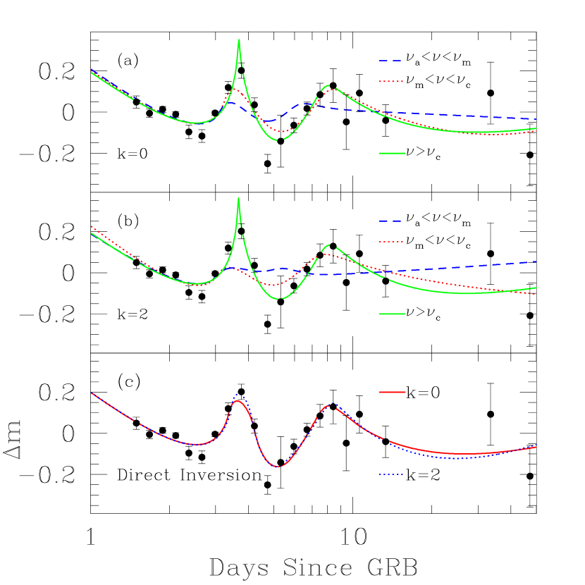
Figure 3: In each panel, the points show the binned residuals from the best-fit double power-law fit (without lensing) in magnitudes. The curves show the difference between microlensing models with various SBPs and the double power law. (a) Theoretically calculated SBPs for k=0. (b) Theoretically calculated SBPs for k=2. (c) SBPs determined from direct inversion.

Model	$-\alpha_{1}$	$-\alpha_{2}$	$s$	$t_{\rm b}$	$b$	$R_{0}$	$\chi^{2}$/dof
No $\mu$-lensing	$0.64_{-0.06}^{+0.05}$	$2.72_{-0.10}^{+0.11}$	$3.14_{-0.91}^{+1.37}$	$4.80_{-0.19}^{+0.21}$	—	—	240.7/93
$k=0$, $\nu_{m}<\nu<\nu_{c}$	$1.07_{-0.02}^{+0.02}$	$2.31_{-0.10}^{+0.23}$	20	$8.14_{-0.48}^{+0.54}$	$0.24_{-0.24}^{+0.23}$	$0.12_{-0.12}^{+0.11}$	166.1/92
$k=0$, $\nu>\nu_{c}$	$1.06_{-0.02}^{+0.02}$	$2.62_{-0.11}^{+0.10}$	20	$7.89_{-0.42}^{+0.49}$	$0.65_{-0.13}^{+0.13}$	$0.29_{-0.06}^{+0.06}$	154.7/92
$k=2$, $\nu>\nu_{c}$	$1.04_{-0.02}^{+0.02}$	$2.63_{-0.11}^{+0.11}$	20	$8.01_{-0.44}^{+0.51}$	$0.60_{-0.12}^{+0.12}$	$0.23_{-0.05}^{-0.05}$	155.5/92
$k=0$, DI	$1.06_{-0.02}^{+0.02}$	$2.60_{-0.10}^{+0.11}$	20	$7.88_{-0.41}^{+0.45}$	$0.62_{-0.19}^{+0.24}$	$0.29_{-0.06}^{+0.07}$	148.5/89
$k=2$, DI	$1.05_{-0.02}^{+0.02}$	$2.51_{-0.10}^{+0.11}$	20	$8.36_{-0.48}^{+0.49}$	$0.44_{-0.40}^{+0.41}$	$0.18_{-0.18}^{+0.13}$	146.9/89
$k=0$, GLS	$1.06_{-0.02}^{+0.02}$	$2.71_{-0.09}^{+0.10}$	$15.5_{-10.0}^{+\infty}$	$7.74_{-0.37}^{+0.37}$	$0.87_{-0.14}^{+0.16}$	$0.41_{-0.08}^{+0.07}$	147.3/89
$k=2$, GLS	$1.05_{-0.02}^{+0.02}$	$2.75_{-0.10}^{+0.10}$	$13.8_{-7.8}^{+\infty}$	$7.68_{-0.36}^{+0.41}$	$0.92_{-0.12}^{+0.15}$	$0.37_{-0.07}^{+0.06}$	146.9/89

Table 1 Fit parameters and $1\sigma$ errors for GRB 000301C.

6 Discussion and Conclusions

We find that the early-time ($t<t_{\rm b}$) flux decline is well-constrained, $\alpha_{1}=-1.05\pm 0.02$. The slope of the optical spectrum at this time is $\beta=-0.9$, taking into account Milky Way (MW) extinction only, but can be as shallow as $\beta=-0.7$ if SMC-type host extinction is included (Rhoads & Fruchter, 2000; Jensen et al., 2001). For $\nu>\nu_{c}$ (the SBPs most consistent with the data), the value of $\alpha_{1}$ implies $p\simeq 2.07$ and thus $\beta=-1.03$, which is only slightly steeper than the observed spectrum for MW extinction. For $\nu_{m}<\nu<\nu_{c}$ and $k=0$, $\alpha_{1}=-1.05$ implies $p=2.4$ and thus $\beta=-0.7$, consistent with observations if SMC-type host extinction is adopted. If the break at $t\sim 8~{}{\rm days}$ is due to a jet, then simple analytic models predict that the change in temporal flux index $\alpha$ should be $\Delta\alpha=(p+3)/4$ for $k=0$ and $\nu_{m}<\nu<\nu_{c}$ or $\Delta\alpha=(p+2)/4$ for $\nu>\nu_{c}$ and $k=0$ or $2$ (Sari, Piran, & Halpern, 1999; Panaitescu & Kumar, 2001). Kumar & Panaitescu (2000) find, using a semi-analytic model, that the jet break is rather smooth, especially for a wind environment ($k=2$), and therefore inconsistent with the sharp break that we infer. However, initial results of numerical calculations of the jet break (Granot et al., 2001), based on a 2D hydrodynamic simulation of the jet for $k=0$, indicate that the break can be rather sharp (with $s\sim 4.5$ for an observer along the jet axis), and that $\alpha_{2}$ is smaller by $\sim 0.35$ compared to the simple analytic predictions mentioned above, making $\Delta\alpha$ larger by a similar factor. Nevertheless, the sharpness of the break still presents a serious problem for the model where the jet propagates into a stellar wind ($k=2$). Also, the SBP is expected to become more uniform at $t>t_{\rm b}$ compares to $t<t_{\rm b}$ (Ioka & Nakamura, 2001; Panaitescu, 2001). Since we assume that the form of the SBP relevant for $t<t_{\rm b}$ holds all along, we underestimate the value of $\alpha_{2}$, and overestimate the value of $\Delta\alpha$ accordingly. This effect is expected to be larger for $\nu>\nu_{c}$, where the SBP is more limb brightened to begin with. The values we obtain for $\Delta\alpha$ may therefore serve as upper limits (especially for $\nu>\nu_{c}$). For the SBP fit for $k=0$ and $\nu_{m}<\nu<\nu_{c}$, we find $\Delta\alpha\lesssim 1.2_{-0.1}^{+0.2}$ whereas based on the electron index derived from $\alpha_{1}$, the prediction is $\Delta\alpha\approx 1.7$. For $\nu>\nu_{c}$ and $k=0$, we find $\Delta\alpha\lesssim 1.56\pm 0.11$, which is reasonably consistent with the prediction $\Delta\alpha\approx 1.37$.

Thus, assuming the break in the light curve is due to jet effects, the only scenario which provides a satisfactory explanation of the data is $\nu>\nu_{c}$ and $k=0$. For $\nu<\nu_{c}$, the inferred SBP is only marginally consistent with the expected profile, and the observed change in the flux indices is smaller than the theoretical expectation. For $\nu>\nu_{c}$ and $k=2$, the observed break is too sharp compared to theoretical predictions. We note that our best fit model parameters, $\nu>\nu_{c}$ and $k=0$, are also favored by Panaitescu (2001), and said to provide a good fit to the data by Berger et al. (2000).

Panaitescu (2001) argued that the expected SBPs are too uniform to reproduce a significant microlensing deviation. This conclusion appears to be partially due to the fact that he found a best-fit impact parameter of $b\sim 2$, whereas we find $b=0.44$–$0.65$ (and $b=0.65$ for our best fit model). All else equal, more uniform SBPs will result in microlensing deviations that are shallower and broader than more limb-brightened SBPs. Thus, to reproduce the observed deviation, a more uniform source must have a smaller impact parameter, a trend we find empirically when fitting the theoretical SBPs. Thus, it is unclear why Panaitescu (2001), who argued that the expected SBPs should be more uniform than that found by GLS, derived a value of $b$ that is twice as large ($b\sim 2$ versus $b\sim 1$).

We conclude that the microlensing of realistic SBPs can explain the optical/infrared light curve of GRB 000301C. Fitting the data with a non-parametric SBP reveals that the afterglow image must be significantly limb-brightened. Specifically, ${{}_{>}\atop{}^{{}^{\sim}}}60\%$ of the flux must originate from the outer 25% of the area of the image (with a significance of $3\sigma$). The recovered SBP is marginally consistent (at the $\sim 3\sigma$ level) with the profile expected for a uniform external density profile ($k=0$) and frequencies $\nu_{m}<\nu<\nu_{c}$. It is consistent at the $\sim 2\sigma$ level with the emission expected from frequencies $\nu>\nu_{c}$ and both uniform ($k=0$) and wind-like ($k=2$) external media.

References

- Berger et al. (2000) Berger, E., et al. 2000, ApJ, 545, 56
- Blandford & McKee (1976) Blandford, R. D., & McKee, C. F. 1976, Phys. Fluids, 19, 1130
- Chevalier & Li (2000) Chevalier, R.A. & Li, Z.Y. 2000, ApJ, 536, 195
- Frail et al. (2000) Frail, D.A., Waxman, E., & Kulkarni, S.R. 2000, ApJ, 537, 191
- Frail et al. (2001) Frail, D.A., et al. 2001, Nature, submitted (astro-ph/0102282)
- Freedman & Waxman (2001) Freedman, D. L., & Waxman, E. 2001, ApJ, 547, 922
- Gaudi & Loeb (2001) Gaudi, B.S., & Loeb, A. 2001, ApJ, 558, 000 (astro-ph/0102003)
- Garnavich, Loeb & Stanek (2000) Garnavich, P.M., Loeb, A., & Stanek, K.Z. 2000, ApJ, 544, L11 (GLS)
- Granot & Loeb (2001) Granot, J., & Loeb, A. 2001, ApJ, 551, L63
- Granot et al. (2001) Granot, J., et al. 2001, to appear in the proceedings of the 2nd workshop on ’Gamma-Ray Bursts in the Afterglow Era’, Rome 2000 (astro-ph/0103038)
- Granot, Piran & Sari (1999a) Granot, J., Piran, T., & Sari, R. 1999a, ApJ, 513, 679
- Granot, Piran & Sari (1999b) ——————————-. 1999b, ApJ, 527, 236
- Granot & Sari (2001) Granot, J., & Sari, R. 2001, in preparation
- Harrison et al. (1999) Harrison, F.A., et al. 1999, ApJ, 523, L121
- Ioka & Nakamura (2001) Ioka, K., & Nakamura, T. 2001, ApJL, in press (astro/ph-0102028)
- Jensen et al. (2001) Jensen, B.L., et al. 2001, A&A, 370, 909
- Koopmans & Wambsganss (2001) Koopmans, L.V.E., & Wambsganss, J. 2001, MNRAS, submitted (astro-ph/0011029)
- Kumar & Panaitescu (2000) Kumar, P., & Panaitescu, A. 2000, ApJ, L541
- Loeb & Perna (1998) Loeb, A., & Perna, R. 1998, ApJ, 495, 597
- Mao & Loeb (2001) Mao, S., & Loeb, A. 2001, ApJ, 547, L97
- Masetti et al. (2000) Masetti, N., et al. 2000, A&A, 359, L23
- Panaitescu (2001) Panaitescu, A. 2001, ApJ, in press (astro-ph/0102401)
- Panaitescu & Kumar (2001) Panaitescu, A., & Kumar, P. 2001, ApJ, in press (astro-ph/0010257)
- Panaitescu & Meszaros (1998) Panaitescu, A., & Meszaros, P. 1998, 493, L31
- Piran (2000) Piran, T. 2000, Physics Reports, 333, 529
- Rhoads & Fruchter (2000) Rhoads, J., & Fruchter, A.S. 2000, ApJ, 546, 117
- Sagar et al. (2000) Sagar, R., Mohan, V., Pandey, S.B., Pandey, A.K., Stalin, C.S., & Tirado, A.J. 2000, BASI, 28, 499
- Sari (1998) Sari, R. 1998, ApJ, 494, L49
- Sari, Piran, & Halpern (1999) Sari, R., Piran, T., & Halpern, T. 1999, ApJ, 519, L17
- Sari, Piran, & Narayan (1998) Sari, R., Piran, T., & Narayan, R. 1998, ApJ, 497, L17
- Stanek et al. (2000) Stanek, K.Z., Garnavich, P.M., Barmby, P., & Jha, S. 2000, BCN Circ. 766 (http://gcn.gsfc.nasa.gov/gcn/gcn3/766.gcn3)
- Van Paradijs et al. (2000) Van Paradijs, J., Kouveliotou, C., & Wijers, R.A.M.J. 2000, ARA&A, 38, 379
- Wijers & Galama (1999) Wijers, R. A. M. J., & Galama, T. J. 1999, ApJ, 523, 177
- Waxman (1997) Waxman, E. 1997, ApJ, 491, L19