Simulations of MHD Turbulence in a Strongly Magnetized Medium

Abstract

We analyze 3D numerical simulations of driven incompressible magnetohydrodynamic (MHD) turbulence in a periodic box threaded by a moderately strong external magnetic field. We sum over nonlinear interactions within Fourier wavebands and find that the time scale for the energy cascade is consistent with the Goldreich-Sridhar model of strong MHD turbulence. Using higher order longitudinal structure functions we show that the turbulent motions in the plane perpendicular to the local mean magnetic field are similar to ordinary hydrodynamic turbulence while motions parallel to the field are consistent with a scaling correction which arises from the eddy anisotropy. We present the structure tensor describing velocity statistics of Alfvenic and pseudo-Alfvenic turbulence. Finally, we confirm that an imbalance of energy moving up and down magnetic field lines leads to a slow decay of turbulent motions and speculate that this imbalance is common in the interstellar medium where injection of energy is intermittent both in time and space.

1 Introduction

The interstellar medium (ISM) is complicated and dynamic. The magnetic field and dynamic pressure ($\rho\,{\bf v}^{2}$/2) usually dominate the thermal pressure ($nkT$), dramatically influencing the star formation rate (see McKee 1999 for a review). There are cosmic rays that provide pressure and heating as well.

One approach to studying the ISM is to perform time-dependent numerical simulations to model the ISM, including as many of the interacting phenomena as practical. Of course, the physics included in such models must necessarily be highly simplified, and it is difficult to determine which features of the final model result from which physical assumptions (or initial conditions). Our approach is to use simplified numerical simulations to study the influences of various physical phenomena in isolation. We want to obtain a physical feeling for the general effects that each phenomenon has on the nature of the ISM. In this paper we will consider the influence of random forces per unit volume on MHD turbulence in an incompressible medium. It is obvious that the real ISM is compressible, but we want to separate the effects of magnetic turbulence from those involving compression. In later papers we will include compression for comparison with the present models, thereby isolating its importance directly.

Historically hydrodynamic turbulence in an incompressible fluid was successfully described by the eddy cascade (Kolmogorov 1941), but MHD turbulence was first modeled by wave turbulence (Iroshnikov 1963, Kraichnan 1965; hereinafter IK). This theory assumes isotropy of the energy cascade in Fourier space, an assumption which has attracted severe criticism (Montgomery & Turner 1981; Shebalin et al. 1983; Montgomery & Matthaeus 1995; Sridhar & Goldreich 1994). Indeed, the magnetic field defines a local symmetry axis since it is easy to mix field lines in directions perpendicular to the local ${\bf B}$ and much more difficult to bend them. The idea of an anisotropic (perpendicular) cascade has been incorporated into the framework of the reduced MHD approximation (Strauss 1976; Rosenbluth 1976; Montgomery 1982; Zank & Matthaeus 1992; Bhattacharjee, Ng, & Spangler 1998).

In a turbulent medium, the kinetic energy associated with large scale motions is greater than that of small scales. However, the strength of the local mean magnetic field is almost the same on all scales. Therefore, it becomes relatively difficult to bend magnetic field lines as we consider smaller scales, leading to more pronounced anisotropy. A self-consistent model of MHD turbulence which incorporates this concept of scale dependent anisotropy was introduced by Goldreich & Sridhar (1995) (henceforth GS95).

Within the GS95 theory the energy cascade becomes anisotropic as a consequence of the resonant conditions for 3-wave interactions. A strict application of the resonant 3-wave interaction conditions gives an energy cascade which is purely in the direction perpendicular to the external field. However, it is intuitively clear that the increase in $k_{\perp}$ must at some point start affecting $k_{\|}$.

The cornerstone of the GS95 theory is the concept of a ‘critically balanced’ cascade, where $k_{\parallel}V_{A}\sim k_{\perp}v_{l}$, where $k_{\perp}$ and $k_{\|}$ are wave numbers perpendicular and parallel to the background field an $v_{l}$ is the r.m.s. speed of turbulence at the scale $l$. In this model, the Alfvén rate ($k_{\parallel}V_{A}$) is equal to the eddy turnover rate ($k_{\perp}v_{l}$). Using this concept, Goldreich & Sridhar showed that the energy cascade is not strictly perpendicular to the background field, but is relaxed so that $k_{\|}\propto k_{\perp}^{2/3}$. Their model predicts that the one-dimensional energy spectrum is Kolmogorov-type if expressed in terms of perpendicular wavenumbers, i.e. $E(k_{\perp})\propto k_{\perp}^{-5/3}$.

Numerical simulations by Cho & Vishniac (2000a, henceforth CV00) and Maron & Goldreich (2001, hereinafter MG01) have mostly supported the GS95 model and helped to extend it. Both analyses stressed the point that scale dependent anisotropy can be measured only in local coordinate frames which are aligned with the locally averaged magnetic field direction. Cho & Vishniac (2000a) calculated the structure functions of velocity and magnetic field in the local frames, and found that the contours of the structure functions do show scale dependent anisotropy, consistent with the predictions of the GS95 model. In their calculation, the strength of the uniform background magnetic field is roughly the same as the the r.m.s. velocity. MG01 tested the GS95 model for a much stronger uniform background field and also obtained results supporting the GS95 model, but they produced $E(K)\propto k^{-3/2}$. They also calculated time scales of turbulence, interactions between pseudo- and shear-Alfvenic modes, growth of imbalance, and intermittency. Other related recent numerical simulations include Matthaeus et al. (1998), Müller & Biskamp (2000), and Milano et al. (2001).

These studies left a number of unresolved issues, including the exact scaling relations, the comparison of intermittency in MHD and in hydrodynamic turbulence, and the time scale of turbulence decay. Moreover, for many practical applications a more quantitative description of MHD turbulence statistics is necessary. These are vital for understanding various astrophysical processes, including star formation (McKee 1999), cosmic ray propagation (Kóta & Jokipii 2000), and magnetic reconnection (Lazarian & Vishniac 1999).

In this paper, we further investigate implications of the GS95 model. In §2, we explain our numerical method. In §3, we further elucidate the scaling relation implied by the GS95 model. In particular, we discuss the time scale, velocity scaling relations, and intermittency. In §4, we derive the correlation tensor and discuss some astrophysical applications. While the GS95 model predicts the MHD turbulence decays in just one eddy turnover time, in §5, we show that the decay time scale increases when the cascade is unbalanced and discuss some consequences of this fact. In §6, we briefly discuss the implications of this work. In §7 we give a summary and our conclusions. As before, we consider the case where the uniform background magnetic field energy density is comparable to the turbulent energy density.

2 Method

2.1 Numerical Method

We have calculated the time evolution of incompressible magnetic turbulence subject to a random driving force per unit mass. We have adopted a pseudospectral code to solve the incompressible MHD equations in a periodic box of size $2\pi$:

$$\frac{\partial{\bf v}}{\partial t}=(\nabla\times{\bf v})\times{\bf v}-(\nabla\times{\bf B})\times{\bf B}+\nu\nabla^{2}{\bf v}+{\bf f}+\nabla P^{\prime},$$ (1)

$$\frac{\partial{\bf B}}{\partial t}=\nabla\times({\bf v}\times{\bf B})+\eta\nabla^{2}{\bf B},$$ (2)

$$\nabla\cdot{\bf v}=\nabla\cdot{\bf B}=0,$$ (3)

where $\bf{f}$ is a random driving force, $P^{\prime}\equiv P/\rho+{\bf v}\cdot{\bf v}/2$, ${\bf v}$ is the velocity, and ${\bf B}$ is magnetic field divided by $(4\pi\rho)^{1/2}$. In this representation, ${\bf v}$ can be viewed as the velocity measured in units of the r.m.s. velocity, v, of the system and ${\bf B}$ as the Alfven speed in the same units. The time $t$ is in units of the large eddy turnover time ($\sim L/v$) and the length in units of $L$, the inverse wavenumber of the fundamental box mode. In this system of units, the viscosity $\nu$ and magnetic diffusivity $\eta$ are the inverse of the kinetic and magnetic Reynolds numbers respectively. The magnetic field consists of the uniform background field and a fluctuating field: ${\bf B}={\bf B}_{0}+{\bf b}$. We use 21 forcing components with $2\leq k\leq\sqrt{12}$, where wavenumber $k$ is in units of $L^{-1}$. Each forcing component has correlation time of one. The peak of energy injection occurs at $k\approx 2.5$. The amplitudes of the forcing components are tuned to ensure $v\approx 1$ We use exactly the same forcing terms for all simulations. The Alfvén velocity of the uniform background field, $B_{0}$, is set to 1. We consider only cases where viscosity is equal to magnetic diffusivity:

$$\nu=\eta.$$ (4)

In pseudo spectral methods, the temporal evolution of equations (1) and (2) are followed in Fourier space. To obtain the Fourier components of nonlinear terms, we first calculate them in real space, and transform back into Fourier space. The average kinetic helicity in these simulations is not zero. However, previous tests have shown that our results are insensitive to the value of the kinetic helicity. In incompressible fluid, $P^{\prime}$ is not an independent variable. We use an appropriate projection operator to calculate $\nabla P^{\prime}$ term in Fourier space and also to enforce divergence-free condition ($\nabla\cdot{\bf v}=\nabla\cdot{\bf B}=0$). We use up to $256^{3}$ collocation points. We use an integration factor technique for kinetic and magnetic dissipation terms and a leap-frog method for nonlinear terms. We eliminate the $2\Delta t$ oscillation of the leap-frog method by using an appropriate average. At $t=0$, the magnetic field has only its uniform component and the velocity field is restricted to the range $2\leq k\leq 4$ in wavevector space.

Hyperviscosity and hyperdiffusivity are used for the dissipation terms (see Table 1). The power of hyperviscosity is set to 8, so that the dissipation term in the above equation is replaced with

$$-\nu_{8}(\nabla^{2})^{8}{\bf v},$$ (5)

where $\nu_{8}$ is determined from the condition $\nu_{h}(N/2)^{2h}\Delta t\approx 0.5$ (see Borue and Orszag 1996) Here $\Delta t$ is the time step and $N$ is the number of grid points in each direction. The same expression is used for the magnetic dissipation term. We list parameters used for the simulations in Table 1. We use the notation XY-$B_{0}$Z, where X = 256, 144 refers to the number of grid points in each spatial direction; Y = H refers to hyperviscosity; Z=1 refers to the strength of the external magnetic field.

Diagnostics for our code can be found in Cho and Vishniac (2000b). For example, our code conserves total energy very well in simulations with $\nu=\eta=0$ and the average energy input (=${\bf f}\cdot{\bf v}$) is almost exactly the same as the sum of magnetic and viscous dissipation in simulations with nonzero $\nu$ and $\eta$. The runs 256H-$B_{0}$1 and 144H-$B_{0}$1 are exactly the same as the runs 256H-$B_{0}$1 and REF2 in CV00. The energy spectra as a function of time for these runs can be found in that paper.

2.2 Defining the Local Frame

The GS95 model deals with strong MHD turbulence and should be distinguished from theories that deal with weak MHD turbulence (e.g. Sridhar & Goldreich 1994; Ng & Bhattacharjee 1996; Galtier et al. 2000; see also Goldreich & Sridhar 1997). In strong MHD turbulence eddy-like motions mix up magnetic field lines perpendicular to the local direction of magnetic field. Thus, as in the case of hydrodynamic turbulence, the correlation time for coherent structures is comparable to the inverse of $k_{\perp}v_{k}$ for any scale $k_{\perp}^{-1}$. These mixing motions are strongly coupled to wave-like motions with a correlation time $(k_{\|}V_{A})^{-1}$. The GS95 model is based on the concept of a ‘critical balance’ between these time scales, that is $k_{\parallel}V_{A}\sim k_{\perp}v_{k}$. . This results in a scale dependent anisotropy, $k_{\|}\propto k_{\perp}^{2/3}$ so that the eddies are increasingly elongated on smaller scales.

The turbulent magnetic field changes its direction in the global system of reference. It is important that the mixing motions are available only in the direction perpendicular to the local direction of magnetic field. Thus the theory must be formulated using the system of reference aligned with the local magnetic field. CV01 discusses in detail one way of defining this system given numerical data.

Figure 1 is a schematic representation of the GS95 model. In Fourier space, the energy injected on large scales excites large scale Fourier components of the magnetic field (the dark region at the center in Fig. 1a). The external magnetic field makes the subsequent energy cascade to small scales anisotropic: it occurs in the directions perpendicular to the mean external field. The GS95 model states that most of the energy is confined to the region $k_{\|}=\pm k_{\perp}^{2/3}$, and as the energy cascades to larger values of $k_{\perp}$ the energy of Fourier components between $k_{\perp}$ and $k_{\perp}+1$ decreases as $E(k_{\perp})\propto k_{\perp}^{-5/3}$.

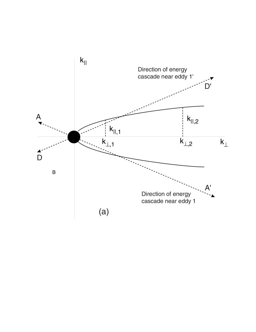
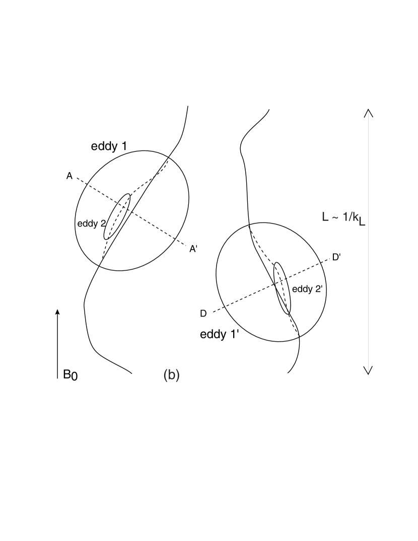
Figure 1: (a) Fourier space structure. (b) Real space structure. Large eddies (eddy $1$ or $1^{\prime}$)) have similar semi-major axis ($\sim 1/k_{\|,1}$) and semi-minor axis ($\sim 1/k_{\perp,1}$). Therefore, they are almost isotropic. Smaller eddies (eddy $2$ or $2^{\prime}$) have relatively larger semi-major axis ($\sim 1/k_{\|,2}$) to semi-minor axis ($\sim 1/k_{\perp,2}$) ratio. Therefore, they are relatively more elongated. Energy cascades in the directions perpendicular to large-scale magnetic field lines (e.g. direction $AA^{\prime}$ or $DD^{\prime}$ in both figure (a) and (b)). This effect obscures scale-dependent anisotropy (e.g. $k_{\|}\propto k_{\perp}^{2/3}$ in GS95 model) when we perform Fourier analysis in the global frame. In Figure (b), the solid curves represent the wandering of magnetic field lines by the large scale magnetic fields. The solid curves can define the directions of the local mean magnetic field line for eddy $1$ or $1^{\prime}$. Similarly, the dashed curves can define the directions of the local mean magnetic field line for the eddy $2$ or $2^{\prime}$.

As illustrated in Fig. 1b, eddies are not aligned along the mean field ${\bf B}_{0}$. Instead, they are aligned along the local mean field lines. The local mean magnetic field defines the physically relevant background for the eddy dynamics, and is determined by the Fourier components whose wavenumbers are a bit less than the characteristic wavenumber of the eddy. In practice, it can be obtained by averaging the magnetic field in the vicinity of the eddy over a volume slightly (say, for example, 2$\times$) larger than the size of the eddy (see CV00 for details). The solid curves in Fig. 1b represent this kind of locally defined mean, formed by all magnetic Fourier components whose scales are a bit larger than eddy 1 (or 1^′). The characteristic scale of this wandering is $L\sim 1/k_{L}$, the energy injection scale, because eddy 1 (or 1^′) is only slightly smaller than the energy injection scale. This large-scale wandering is smooth but dominates over smaller scale effects because the the magnetic energy is concentrated on larger scales. Wandering by smaller scale magnetic fields is weaker and causes smaller deviations from the large-scale wandering. We depict the additional wandering caused by scales a bit larger than the eddy 2 as a dashed curve in Figure 1b. For the eddy 1, the solid curve defines the local mean magnetic field and, for the eddy 2 the dashed curve.

The GS95 model is dominated by local dynamics, that is, in this model disturbances lose their coherence when propagating over a single wavelength. To the extent that the dynamics are local it is obvious that the only relevant magnetic field is the local mean field. As an example, consider eddies 1 and 2 in Figure 1b again. For eddy 1, the solid curve can be regarded as a local mean field line and the energy cascade will take place perpendicular to this field, along the direction $AA^{\prime}$. Smaller eddies, like eddy 2 sees the dashed curve as its local background magnetic field with a slightly different direction for the energy cascade. Since the difference between the two curves is small, the direction of the energy cascade differs only slightly as a function of scale. Basically, energy cascades along $AA^{\prime}$ in the region near the eddy 1. Similarly, energy cascades along $DD^{\prime}$ in the region near the eddy 1^′. We are left with an energy cascade which differs both as a function of scale and as a function of location. However, the dynamics are not entirely local, in the sense that disturbances do propagate along field lines without retaining phase coherence. Consequently, perpendicular motions in eddy 1 can lead to similar motions in eddy 1^′, even though $AA^{\prime}$ and $DD^{\prime}$ are not parallel vectors. This is one of the key features of the GS95 model, and carries with it the implication is that dynamic variables need to be evaluated in terms of the local mean field direction, rather than a global coordinate system. Conversely, the ability to generate a more meaningful description in terms of a local, and scale-dependent, coordinate system can be taken as an indirect confirmation of some features of the GS95 model.

In summary, when we want to describe the scaling of eddy shapes, we should correctly identify the direction of the local mean magnetic field. When we talk about anisotropy, we talk about anisotropy with respect to local mean magnetic field lines. Because of this, it is necessary to introduce a ‘local’ frame in which the direction of the local mean magnetic field lines is taken as the parallel direction. When we consider the GS95 picture (i.e. $k_{\|}\propto k_{\perp}^{2/3}$) in Fourier space, we are considering the local frame in real space, and vice versa. When we describe turbulence with respect to the global frame, which is fixed in real space, the corresponding Fourier space structure no longer shows the GS95 picture. Instead, we have a relation close to $k_{\|}\propto k_{\perp}$. This is because when energy cascades along $AA^{\prime}$, $DD^{\prime}$, or some intermediate directions in real space (Fig 1b), it cascades along the directions between $AA^{\prime}$ and $DD^{\prime}$ in Fourier space (Fig 1a), which implies that, when we perform the Fourier transform with respect to the fixed global frame, we will get $k_{\|}\propto k_{\perp}$. The true scaling relation is eclipsed by the wandering of large scale magnetic field lines.

It is very important to identify the local frame. In this paper, when we calculate decay time scale, intermittency, and the correlation tensor, we always refer to the local frame.

3 Scaling Relations

3.1 Time Scale of Motions

One of the basic questions in the theory of MHD turbulence is the slope of the one-dimensional energy spectra. As we have seen, GS95 obtained a spectral index of $-5/3$. In the numerical simulations of CV00 the spectral index is close to $-5/3$, while it is very close to $-3/2$ in MG01. The IK theory predicts a $k^{-3/2}$ scaling, although the other features of this model are definitely inconsistent with all the numerical evidence. MG01 attributed their result to the appearance of strong intermittency in their simulations. We note that the inertial range of the solar wind shows a spectral index of $-1.7$ (Leamon et al. 1998; see also Matthaeus & Goldstein 1982), but this number should be considered cautiously. The physics of the solar wind is undoubtedly more complicated than the simulations described here.

Can we test which scaling is correct? The cascade time as function of scale presents us with an interesting constraint.

IK theory and GS95 model predict different scalings for turbulent cascade time scale ($t_{cas}$). In both theories, $t_{cas}$ can be determined by the scale-independence of the cascade:

$$v^{2}_{k}/t_{cas}=\mbox{constant}.$$ (6)

Since $v^{2}_{k}$ is proportional to $kE(k)$, we have

$$t_{cas,IK}\propto k^{-1/2},~{}~{}~{}~{}t_{cas,GS}\propto k^{-2/3}$$ (7)

for IK theory and GS95 model respectively. This result is also useful for certain intermittency theories (see §3.3). MG01 studied the cascade time scale using three different methods and obtained slopes comparable to $-2/3$ (i.e. $t_{cas}\propto k_{\perp}^{-2/3}$) in two methods and $-1/2$ in the other method.

Here we consider a different method of evaluating $t_{cas}$. The purpose of our calculation is to test MG01’s result using another numerical method and demonstrate the effects of large scale fluid motions on the calculation of $t_{cas}$.

Symbolically, we can rewrite the MHD equations as follows:

$$\dot{\bf v}_{\bf k}=N^{v}_{\bf k},$$ (8)

$$\dot{\bf b}_{\bf k}=N^{b}_{\bf k},$$ (9)

where $N^{v}$ and $N^{b}$ represent the nonlinear terms. We have ignored the dissipation terms. Naively speaking, we might obtain the time scale by dividing $|{\bf v}_{\bf k}|$ by $|N^{v}_{\bf k}|$. However, this gives $t_{cas}\propto k^{-1}$, where the exponent is almost exactly $-1$. This is not actually a measure of the cascade time. We note that CV00 obtained a similarly misleading relation for the cascade time, and attributed it to the effect of large scale translational motions. Although they used a different method to calculate the cascade time, the same argument applies here. If we consider the interaction between a small eddy and a large scale (translational) fluid motion, then the translation can be removed by a Galilean transformation, and there is no associated energy cascade. However, the phase of the Fourier components that represent the small eddy is affected by the large scale translational motion, and changes at a rate kV, where $V$ is the large scale velocity. The corresponding nonlinear term has a magnitude of $|N_{k}|\sim|{\bf v}_{k}|kV$, which accounts for the (misleading) relation $t_{cas}\sim k^{-1}$. The cascade time as a function of wavenumber can be evaluated directly from our simulations, but only after we filter out translational motions arising from eddies much larger than the scale under consideration.

We correct for the presence of large scale motions by restricting the evaluation of the nonlinear terms to contributions coming from the interactions between the mode at $k$ and other modes within the range of $k/2$ and $2k$. In doing this, we retain the uniform magnetic component $B_{0}$. We show the result in Figure 2. Our result supports the GS95 model: $t_{cas}\propto k^{-2/3}$. In comparison with MG01 we obtained this result using a different method and for a different kinetic/magnetic energy ratio.

In the GS95 model, $t_{cas}$ is determined by the relation $t_{cas}\sim l_{\perp}/v_{l\perp}$. This means that the cascade time scale is virtually synonymous with the eddy turnover time, which is also true for hydrodynamic turbulence. It is obvious that the cascade time determines the decay time scale of turbulence. As a consequence, the GS95 model implies that MHD turbulence decays as fast as hydrodynamic turbulence (say, $t_{decay}$= a few eddy turnover times). Note that no matter how strong the external field is, strong MHD turbulence decays within a few eddy turn over times. We discuss the implications of this result, and some limitations, in §5.

These results support the original GS95 theory. However, we are not in a position to directly confront the results of MG01. Our simulations differ from theirs in many ways, including the shape of the computational box, the range of length scales, and the strength of the uniform background field. We shall address those issues elsewhere. In §3.3, we will discuss what the study of intermittency implies about the slope of energy spectra.

Figure 2: Cascade time scale. The GS95 model predicts $t_{cas}\propto k^{-2/3}$, while the IK theory predicts $t_{cas}\propto k^{-1/2}$. Our result supports the GS95 model. Run 256H-$B_{0}$1.

Figure 3: Second-order structure functions. Across local mean magnetic field lines, the second-order structure functions follow $r^{2/3}$. Along the local mean magnetic field lines, they follow $r^{1}$. For pseudo-Alfven modes this defines the scaling of motions parallel to local mean magnetic field lines. $VSF_{2}$ and $BSF_{2}$ denote the second order structure functions for velocity and magnetic field respectively. Run 256H-$B_{0}$1.

3.2 Velocity Scaling

In the GS95 model, $v_{\perp}^{2}$ is proportional to $\sim k_{\perp}E(k_{\perp})$, where $E(k_{\perp})$ is the one-dimensional energy spectrum. Since $E(k_{\perp})\propto k_{\perp}^{-5/3}$, we have $v_{\perp}^{2}\propto l_{\perp}^{2/3}$ or $SF_{2}(l_{\perp},0)\propto l_{\perp}^{2/3}$, where $SF_{2}$ is the second order structure function:

$$SF_{2}(l_{\perp},l_{\|})=<\left[{\bf v}({\bf x}+{\bf l})-{\bf v}({\bf x})\right]^{2}>,$$ (10)

where the angle brackets denote the spatial average over x and ${\bf l}=l_{\perp}{\bf e}_{\perp}+l_{\|}{\bf e}_{\|}$. The vectors ${\bf e}_{\perp}$ and ${\bf e}_{\|}$ are unit vectors perpendicular and parallel to ${\bf B}_{L}$ respectively. The vector ${\bf B}_{L}$ denotes the local mean magnetic field.

What can we say about the velocity scaling parallel to ${\bf B}_{L}$? We can consider two different quantities. First, we can consider the scaling of Alfven components in the direction parallel to ${\bf B}_{L}$. Second, we can also consider the scaling of pseudo-Alfvenic components along the direction of ${\bf B}_{L}$. The pseudo-Alfvenic components are incompressible limit of slow magnetosonic waves. While they have the same dispersion relations as the Alfven modes, the velocities $v_{l}$ of polarization are completely different: the directions lie in the plane determined by ${\bf B}_{0}$ and ${\bf k}$. Note that the Alfven modes have velocities perpendicular to the plane determined by ${\bf B}_{0}$ and ${\bf k}$.

There are several ways to derive the scaling relation for Alfvenic turbulence from the GS95 model. First, suppose that the second order structure function along local ${\bf B}_{L}$ follows a power law: $SF_{2}(0,l_{\|})\propto l_{\|}^{m}$. When we equate $SF_{2}(0,l_{\|})$ and $SF_{2}(l_{\perp},0)$, we should retrieve the GS95 scaling relation, $l_{\|}\propto l_{\perp}^{2/3}$ (see MG01). We conclude that $m=1$ and $SF_{2}(0,l_{\|})\propto l_{\|}$. Since $k_{\|}E^{v}(k_{\|})~{}(\propto v_{\|}^{2})\propto SF_{2}(l_{\|},0)$, we have $E^{v}(k_{\|})\propto k_{\|}^{-2}$. Alternatively, we can write

$$E_{3}^{v}(k_{\perp},k_{\|})\propto k_{\perp}^{-10/3}g(k_{\|}/k_{\perp}^{2/3}),$$ (11)

where $E_{3}^{v}(k_{\perp},k_{\|})$ is the 3-dimensional energy spectrum and $g$ is a function which describes distribution of energy along $k_{\|}$ direction in Fourier space. We will give a reasonable fit to its functional form in the next section.

We plot our results in Figure 3, in which we observe that $SF_{2}(l_{\perp},0)$ (across ${\bf B}_{L}$) $\propto l_{\perp}^{2/3}$ and $SF_{2}(0,l_{\|})$ (parallel to ${\bf B}_{L}$) $\propto l_{\|}$. The velocity field follows these relations quite well, while the magnetic field follows a slightly different relation across ${\bf B}_{L}$. Both Alfvenic and pseudo-Alfvenic components follow similar scalings in the directions parallel to ${\bf B}_{L}$ In section 4 we shall also show that the 3D spectrum of pseudo-Alfven motions has a form similar to (11). On this basis we conclude that the scaling $E^{v}(k_{\|})\propto k_{\|}^{-2}$ also applies to pseudo-Alfven motions, where the velocities are mostly parallel to the local mean magnetic field ${\bf B_{L}}$. The corresponding velocities $v_{\|}^{2}\propto k_{\|}E^{v}(k_{\|})$ which means that $v_{\|}^{2}\propto k_{\|}^{-1}\propto l_{\|}$. This result is important for many problems, including dust transport (Yan et al 2001). Note that the energy spectrum is steeper when expressed as a function of the parallel direction.

In this subsection we extended the GS95 model for the parallel motions and pseudo-Alfven modes and confirmed it through numerical simulations.

3.3 Intermittency

MG01 studied the intermittency of dissipation structures in MHD turbulence using the fourth order moments of the Elsasser fields and the gradients of the fields. Their simulations show strong intermittent structures. We use a different, but complementary, method to study intermittency, based on the higher order longitudinal structure functions. Our result is that by this measure the intermittency of velocity field in MHD turbulence across local magnetic field lines is as strong, but not stronger, than in hydrodynamic turbulence.

In fully developed hydrodynamic turbulence, the (longitudinal) velocity structure functions $S_{p}=<([{\bf v}({\bf x}+{\bf r})-{\bf v}({\bf x})]\cdot\hat{\bf r})^{p}>\equiv<\delta v_{L}^{p}({\bf r})>$ are expected to scale as $r^{\zeta_{p}}$. For example, the classical Kolmogorov phenomenology (K41) predicts $\zeta_{p}=p/3$. The (exact) result for p=3 is the well-known 4/5-relation: $<\delta v_{L}^{p}({\bf r})>=-(4/5)\epsilon r$, where $\epsilon$ is the energy injection rate (or, energy dissipation rate). On the other hand, She & Leveque (1994, hereinafter S-L) proposed a different scaling relation: $\zeta_{p}^{SL}=p/9+2[1-(2/3)^{p/3}]$. Note that She-Leveque model also implies $\zeta_{3}=1$.

So far in MHD turbulence, to the best of our best knowledge, there is no rigorous intermittency theory which takes into account scale-dependent anisotropy. Therefore, we will use an intermittency model based on an extension of a hydrodynamic model. Politano & Pouquet (1995) have developed an MHD version of She-Leveque model:

$$\zeta_{p}^{PP}=\frac{p}{g}(1-x)+C\left(1-(1-x/C)^{p/g}\right),$$ (12)

where $C$ is the co-dimension of the dissipative structure, $g$ is related to the scaling $v_{l}\sim l^{1/g}$, and $x$ can be interpreted as the exponent of the cascade time $t_{cas}\propto l^{x}$. (In fact, $g$ is related to the scaling of Elsasser variable z: $z_{l}\sim l^{1/g}$.) In the framework of the IK theory, where $g=4$, $x=1/2$, and $C=1$ when the dissipation structures are sheet-like, their model of intermittency becomes $\zeta_{p}^{IK}=p/8+1-(1/2)^{p/4}$. On the other hand, Müller & Biskamp (2000) performed numerical simulations on decaying isotropic MHD turbulence and obtained Kolmogorov-like scaling ($E(k)\sim k^{-5/3}$ and $t\sim l^{2/3}$) and sheet-like dissipation structures, which implies $g=3$, $C=1$, and $x=2/3$. From equation (12), they proposed that

$$\zeta_{p}^{MB}=p/9+1-(1/3)^{p/3}.$$ (13)

How does anisotropy change intermittency? We have determined the scaling exponents numerically, working in the local frame. We performed a simulation with a grid of $144^{3}$ collocation points and integrated the MHD equations from t=75 to 120. We calculated the higher order velocity structure functions for 75 evenly spaced snapshots. We average over 5 consecutive values since the correlation time of the turbulence corresponds to 5 snapshots. We calculated the scaling exponents from these averaged structure functions. We obtained a total of 15 (=75/5) such structure functions and scaling exponents. We believe these 15 data sets are mutually independent. We plot the result in Figure 4a. The filled circles represent the scaling exponents of longitudinal velocity structure functions in directions perpendicular to the local mean magnetic field. It is surprising that the scaling exponents are close the original (i.e. hydrodynamic) S-L model. This raises an interesting question. In our simulations, we clearly observe that $t_{cas}\propto l^{2/3}$ and $E(k)\propto k^{-5/3}$. It is evident that MHD turbulence has sheet-like dissipation structures (Politano, Pouquet & Sulem 1995). Therefore, the parameters for our simulations should be the same as those of Müller & Biskamp’s (i.e. $g=3$, $C=1$, and $x=2/3$) rather than suggesting $C=2$. We believe that this difference stems from the different simulation settings: their turbulence is isotropic and ours is anisotropic. In fact, we expect the the small scale behavior of MHD turbulence should not depend on whether or not the largest scale fields are uniform or have the same scale of organization as the largest turbulent eddies. Nevertheless, given the limited dynamical range available in these simulations, it would not be surprising if the scale of the magnetic field has a dramatic impact on the intermittency statistics. It is not clear how scale-dependent anisotropy changes the intermittency model in equation (12) and we will not discuss this issue further. Instead, we simply stress that we have found a striking similarity between ordinary hydrodynamic turbulence and MHD turbulence in perpendicular directions. MG01 attributes the deviation of their spectrum from the Kolmogorov-type to the turbulence intermittency present in the MHD case. Since we do not reproduce their power spectrum, the fact that our intermittency statistics do not support this conjecture is unsurprising. Clearly more studies of the issue are necessary.

Figure 4: (a) Intermittency. Our result (denoted by the filled circles) suggests that MHD turbulence looks like ordinary hydrodynamic turbulence when viewed across the local field lines. SL represents the original She-Leveque model for ordinary hydrodynamic turbulence. IK and MB stand for the IK theory and the Müller-Biskamp model respectively. Error bars are for 1-$\sigma$ level. Run 144H-B₀1. (b) The second, third, and fifth order longitudinal velocity structure functions. These are structure functions averaged over the time interval (75,120).

In figure 4a, we also plot the scaling exponents (represented by filled squares) of longitudinal velocity structure functions along directions of the local mean magnetic field. Although we show only the exponents of longitudinal structure functions, those of transverse structure functions follow a similar scaling law. It is evident that intermittency along the local mean magnetic field directions is completely different from that of previous (isotropic) models. Roughly speaking, the scaling exponents along the directions of local magnetic field are 1.5 times larger than those of perpendicular directions. Interestingly this result implies anisotropy becomes scale independent under the following transformation: $(r_{\perp},r_{\|})\rightarrow(r_{\perp},r_{\|}^{2/3})$. This is consistent with the idea that eddies are stretched along the directions of the local mean magnetic field - if we shrink them in the scale-dependent manner described above along the local field lines, the result is similar to ordinary hydrodynamic turbulence. In this interpretation it is not surprising that MHD turbulence looks similar to ordinary hydrodynamic turbulence across the local mean magnetic field lines - the scaling relation in perpendicular directions is not affected by the local mean magnetic field. Clearly this result is hard to explain using previous models, for example the IK theory. The error bars are larger for parallel directions because fewer number of pairs are available for calculation of the structure functions in these directions than perpendicular directions.

In Figure 4b, we plot average longitudinal velocity structure functions. The slope of the third order structure function is very close to 1. The third order structure function is slightly different from the one discussed earlier in that we calculate $<|\delta v_{L}|^{3}({\bf r})>$ instead of $<(\delta v_{L})^{3}({\bf r})>$.

The second order exponent $\zeta_{2}$ is related to the the 1-D energy spectra: $E(k_{\perp})\propto k_{\perp}^{-(1+\zeta_{2})}$. Previous 2-D driven MHD calculations for $B_{0}=0$ by Politano, Pouquet, & Carbone (1998) also found $\zeta_{2}\sim 0.7$. However, Biskamp, & Schwarz (2001) obtained $\zeta_{2}\sim 0.5$ from decaying 2-D MHD calculations with $B_{0}=0$. Our result suggests that $\zeta_{2}$ is closer to $2/3$, rather than to $1/2$. (It is not clear whether or not the scaling exponents follow the original S-L model exactly. At the same time, our calculation shows that the original S-L model can be a good approximation for our scaling exponents. The S-L model predicts that $\zeta_{2}\sim 0.696$.) Therefore, our result supports the scaling law $E(k_{\perp})\propto k_{\perp}^{-5/3}$ at least for velocity. For the parallel directions, the results support $E(k_{\|})\propto k_{\|}^{-2}$ although the uncertainty is large.

4 The MHD Fluctuation Tensor

For many purposes, e.g. cosmic ray propagation and acceleration, heat transfer etc., it is necessary to know the tensor describing the statistics of magnetic and velocity field. For those applications the one-dimensional spectrum described in MG01 is not adequate and a more detailed description is necessary.

General second-rank correlation tensors are important tools in the statistical description of turbulence. Oughton, Radler, & Matthaeus (1997) gave a comprehensive formalism for the tensors for MHD turbulence and we use their results as a starting point of our argument. Consider the velocity correlation tensor

$$R^{v}_{ij}=<v_{i}({\bf x})v_{j}({\bf x}+{\bf r})>,$$ (14)

where the angle brackets denotes an appropriate ensemble average. The Fourier transform of this tensor is

$$S^{v}_{ij}=<\hat{v}_{i}({\bf k})\hat{v}_{j}^{*}({\bf k})>,$$ (15)

where the asterisk denotes complex conjugate. We can rewrite equation (20) of Oughton et al. (1997) as

$$S_{ij}^{v}=\left[\delta_{ij}-\frac{k_{i}k_{j}}{k^{2}}\right]E^{v}({\bf k})+\left[[e_{i}k_{j}+e_{j}k_{i}]({\bf e}\cdot{\bf k})-e_{i}e_{j}k^{2}-\frac{k_{i}k_{j}}{k^{2}}({\bf e}\cdot{\bf k})^{2}\right]F^{v}({\bf k})+X_{ij},$$ (16)

where $E^{v}({\bf k})$ is (3D) kinetic energy spectrum of all (shear + pseudo) modes, $F^{v}({\bf k})$ is the difference of shear-Alfvén energy and pseudo-Alfvén energy at wave vector ${\bf k}$ divided by $k_{\perp}^{2}$, ${\bf e}$ is a unit vector along ${\bf B}_{0}$, and $X_{ij}=-i[\delta_{i\mu}\epsilon_{j\alpha\beta}+\delta_{j\mu}\epsilon_{i\alpha\beta}]e_{\alpha}k_{\beta}(e_{\mu}k^{2}-k_{\mu}{\bf e}\cdot{\bf k})C^{v}+i\epsilon_{ij\alpha}k_{\alpha}H^{v}$ is a term that describes deviation from mirror symmetry. In this paper we consider axisymmetric turbulence (caused by ${\bf B}_{0}$) with mirror symmetry so that $X_{ij}\equiv 0$. We need only two scalar generating functions, $E^{v}$ and $F^{v}$, for the correlation tensor. This is consistent with Chandrasekhar (1951; see also Oughton et al. 1997).

In this subsection, we will show that the tensor is suitably described by

$$S_{ij}=A_{1}\left[\delta_{ij}-\frac{k_{i}k_{j}}{k^{2}}\right]k_{\perp}^{-10/3}\exp\left(-A_{2}\frac{k_{\|}}{k_{\perp}^{2/3}}\right),$$ (17)

where $A_{1}\sim B_{0}^{2}/L^{1/3}$ and $A_{2}\sim L^{1/3}$ are parameters.

First, we choose ${\bf e}$=(0,0,1), the direction of ${\bf B}_{0}$. Then, equation (16) becomes

$$S_{ij}^{v}=\left[\delta_{ij}-\frac{k_{i}k_{j}}{k^{2}}\right]E^{v}({\bf k})+\left[[\delta_{3i}k_{j}+\delta_{3j}k_{i}]k_{3}-\delta_{3i}\delta_{3j}k^{2}-\frac{k_{i}k_{j}}{k^{2}}k_{3}^{2}\right]F^{v}({\bf k}).$$ (18)

In the absence of anomalous damping of the pseudo-Alfvén modes, as in our simulations, we can show that $F$ in above expression is negligibly small. Note that $F=(S-P)/k_{\perp}^{2}$, where $S$ and $P$ are the squares of the amplitudes of the shear- and pseudo-Alfvén modes (i.e. 3D energy spectra). To evaluate $S$ and $P$, we measured their strength in global frame. (It is non-trivial to correctly define Alfvén modes and pseudo-Alfvén modes in the local frame.) Figure 5 shows that they have similar strengths. We assume that the same relation holds true in the local frame. Since $F$ is the difference between $S$ and $P$, it follows that $F({\bf k})$ is small compared with $E({\bf k})$.

In the previous paragraph, we assumed that there is no special damping mechanism for the pseudo-Alfvén modes. However, it is known that pseudo-Alfvén modes in the ISM are subject to strong damping due to free streaming of collisionless particles along the field lines (Barnes 1966; Minter & Spangler 1997). When the pseudo-Alfvén modes are absent, equation (16) becomes

$$S_{ij}^{v}=\left[\delta_{ij}-\frac{k_{i}k_{j}}{k^{2}}\right]E^{v}({\bf k})+\left[[\delta_{3i}k_{j}+\delta_{3j}k_{i}]k_{3}-\delta_{3i}\delta_{3j}k^{2}-\frac{k_{i}k_{j}}{k^{2}}k_{3}^{2}\right]\frac{E^{v}({\bf k})}{k_{\perp}^{2}}.$$ (19)

For $i,j=1,2$, this becomes $S_{ij}=(\delta_{ij}-k_{i}k_{j}/k^{2})E-(k_{i}k_{j}/k^{2})(k_{\|}/k_{\perp})^{2}E\approx(\delta_{ij}-k_{i}k_{j}/k^{2})E$. And, it is easy to show that $S_{i3}=S_{3i}=0.$ This is easily understood when we note that shear-Alfvén waves do not have fluctuations along ${\bf B}_{0}$.

In summary, the tensor reduces to

$$\left(\begin{array}[]{ccc}(1-k_{1}^{2}/k^{2})E&-(k_{1}k_{2}/k^{2})E&-(k_{1}k_{3}/k^{2})E\\ -(k_{1}k_{2}/k^{2})E&(1-k_{2}^{2}/k^{2})E&-(k_{2}k_{3}/k^{2})E\\ -(k_{1}k_{3}/k^{2})E&-(k_{2}k_{3}/k^{2})E&(1-k_{3}^{2}/k^{2})E\\ \end{array}\right)$$ (20)

for turbulence with both Alfvénic and pseudo-Alfvénic components, and

$$\left(\begin{array}[]{ccc}(1-k_{1}^{2}/k^{2})E&-(k_{1}k_{2}/k^{2})E&0\\ -(k_{1}k_{2}/k^{2})E&(1-k_{2}^{2}/k^{2})E&0\\ 0&0&0\\ \end{array}\right)$$ (21)

for shear Alfvénic turbulence. In equation (21), $E$ stands for the energy of Alfven components only, which is roughly one half of the $E$ in equation (20).

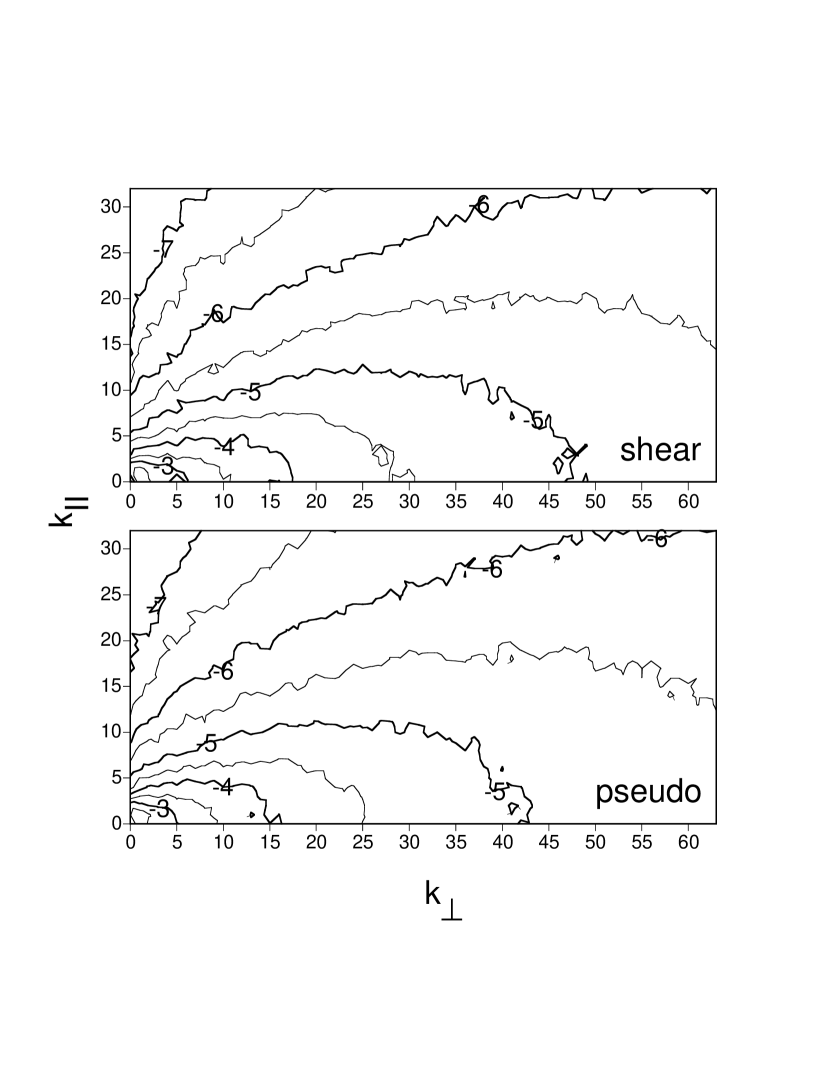
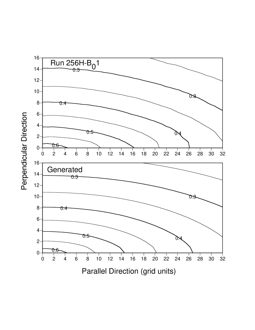
Figure 5: Energy distribution of shear- and pseudo-Alfvén waves. They have similar energy distributions in Fourier space (global frame). Run 256H-$B_{0}$1. Numbers by the contours are $\log_{10}(E_{3}({\bf k}))$.

Figure 6: Upper panel: velocity correlation function from simulations. Lower panel: velocity correlation function generated using the tensor in equation (23). Parallel and perpendicular directions are taken with respect to local mean magnetic field.

The remaining issue is the form of $E$. Note that the trace of $S_{ij}^{v}$ is $2E^{v}$. In real space, the trace is the velocity correlation function. Consequently, we can obtain $E^{v}$ through a FFT of the real-space velocity correlation function, which is directly available from our data cube. However, the velocity correlation function in real space contains considerable numerical noise. In order to minimize its effects while obtaining an empirically useful form for $E$ we first guess $E^{v}$ in Fourier space, do the FFT transform, and then compare the transformed result with the actual velocity correlation function. Since the trace of $S_{ij}^{v}$ is the (3-dimensional) energy spectrum in Fourier space, we start with the original expression in Goldreich & Sridhar (1995) given by equation (11):

$$E_{3}(k_{\perp},k_{\|})\sim\frac{B_{0}^{2}}{k_{\perp}^{10/3}L^{1/3}}g(L^{1/3}\frac{k_{\|}}{k_{\perp}^{2/3}}),$$ (22)

where the functional form of $g(y)$ was not specified. We have tried several functional forms for $g$ ; Gaussian ($g\propto\exp(-Bk_{\|}^{2}/k_{\perp}^{4/3})$), exponential ($\exp(-Bk_{\|}/k_{\perp}^{2/3})$), and a step function. We have found that an exponential form for $g$ gives the best result (Figure 6). Fig 6a is the actual data we obtained from our simulation and Fig 6b is the Fourier-transformed velocity correlation function. Note the similarity of the contours in both plots. We conclude that the tensor can be suitably described by equation (20) or (21) with

$$E(k_{\perp},k_{\|})=(B_{0}/L^{1/3})k_{\perp}^{-10/3}\exp\left(-L^{1/3}\frac{k_{\|}}{k_{\perp}^{2/3}}\right),$$ (23)

where $k_{\perp}$ and $k_{\|}$ should both be interpreted as the absolute magnitudes of those wavevector components.

However, it is worth noting a clear limitation of equation (23): it has a discontinuous derivative near $k_{\|}=0$. One way to overcome this difficulty is to use the Castaing function (Castaing, Gagne & Hopfinger 1990)

$$\Pi_{\lambda}(u)=\frac{1}{2\pi\lambda}\int_{0}^{\infty}\exp\left(-\frac{u^{2}}{2\sigma^{2}}\right)\exp\left(-\frac{\ln^{2}(\sigma/\sigma_{0})}{2\lambda^{2}}\right)\frac{d\sigma}{\sigma^{2}},$$ (24)

which is smooth near zero but looks exponential over a broad range. It is possible to see that for $\lambda=1$ and $\sigma_{0}=k_{\perp}^{2/3}/L^{1/3}$,

$$\exp\left(-L^{1/3}\frac{k_{\|}}{k_{\perp}^{2/3}}\right)\approx\frac{1}{2\pi}\int_{0}^{\infty}\exp\left(-\frac{k_{\|}^{2}}{2\sigma^{2}}\right)\exp\left(-\frac{\ln^{2}(L^{1/3}\sigma/k_{\perp}^{2/3})}{2}\right)\frac{d\sigma}{\sigma^{2}}$$ (25)

However, for many practical applications, we feel that the expression in equation (23) is adequate. For instance, in a forthcoming paper (Yan et al. 2001) this tensor is used for describing cosmic ray propagation and we find a strong suppression of cosmic ray scattering compared with the generally accepted estimates (for example, Schlickeiser 1994). However, if the behavior around $k_{\|}$ is important, the Castaing function would be preferred. In our simulations there is no way to distinguish between exponential and Castaing distributions.

5 Decay of MHD Turbulence

Turbulence plays a critical role in molecular cloud support and star formation and the issue of the time scale of turbulent decay is vital for understanding these processes.

If MHD turbulence decays quickly then serious problems face researchers attempting to explain important observational facts, i.e. turbulent motions seen within molecular clouds without star formation (see Myers 1999) and rates of star formation (Mckee 2000). Earlier studies attributed the rapid decay of turbulence to compressibility effects (Mac Low 1999). Our present study, as well as earlier ones (CV00, MG01), shows that turbulence decays rapidly even in the incompressible limit. This can be understood in the framework of GS95 model where mixing motions perpendicular to magnetic field lines form hydrodynamic-type eddies. Such eddies, as in hydrodynamic turbulence, decay in one eddy turnover time.

How grave is this problem? Some possibilities for reconciling theory with observations were studied earlier. For instance, some problems may be alleviated if the injection of energy happens on the large scale, the eddies are huge, and the corresponding time scales, are much longer (see Lazarian 1999). The fact that the turbulence decays according to a power-law, rather than exponentially, also helps. Indeed, if turbulent energy decays as $t^{-1}$, as suggested by Mac Low wt al. (1998), a substantial level of turbulence should persist after 4-5 turnover times.

There is, however, another property of astrophysical turbulence related to the peculiar nature of the energy injection. It is accepted that sources of interstellar turbulence are localized. As a result, there is a substantial imbalance between the ingoing and outgoing energy flux surrounding every source. Below we consider the effect of this imbalance on the turbulence decay time scale.

For an imbalanced turbulence, it is useful to consider the Elsasser variables, ${\bf z}^{\pm}={\bf v}\pm{\bf b}$, which describe wave packets traveling in opposite directions along the magnetic field lines. Imbalanced turbulence means that wave packets traveling in one direction (say, ${\bf z}^{+}$) have significantly larger amplitudes than the other. In astronomy, many energy sources are localized. For example, SN explosions and OB winds are typical point energy sources. Furthermore, astrophysical jets from YSOs are believed to be highly collimated. With these localized energy sources, it is natural to think that interstellar turbulence is typically imbalanced. In fact, the concept of an imbalanced cascade is not new. Earlier papers (e.g., Matthaeus, Goldstein & Montgomery 1983; Ting, Matthaeus & Montgomery 1986; Ghosh, Matthaeus & Montgomery 1988) have addressed the role and evolution of cross-helicity ($\equiv{\bf v}\cdot{\bf b}$). Since $4<{\bf v}\cdot{\bf b}>=<({\bf z}^{+})^{2}>-<({\bf z}^{-})^{2}>$, non-zero cross-helicity implies an imbalanced turbulent cascade. These works, however, were mainly concerned with the growth of imbalance in decaying turbulence. Ghosh et al. (1988) investigated the evolution of cross-helicity and various spectra in driven turbulence. Hossain et al. (1995) discussed the effects of cross helicity and energy difference $D=<v^{2}>-<b^{2}>$ on the decay of turbulence. Their low resolution 3D numerical simulations show the effect of cross helicity, although that effect is not very conspicuous. A further study of imbalanced turbulence was given in MG01, who also suggested a connection between spontaneous appearance of local imbalance in the turbulent cascade and intermittency in MHD turbulence.

In this subsection, we explicitly relate the degree of imbalance and the decay time scale of turbulence in the presence of a strong uniform background field.

Figure 7: (a) Decay of unbalanced turbulence. Imbalanced cascade can extend decay time. It is clear that the decay of turbulence depends on the degree of imbalance. Run 144H-$B_{0}$1. (b) Same as (a). Log-log scale. Note that about 3 time units is one eddy turn over time.

In Figure 7 we demonstrate that an imbalanced cascade does extend the lifetime of MHD turbulence. We use the run 144H-$B_{0}$1 to investigate the decay time scale. We ran the simulation up to t=75 with non-zero driving forces. Then at t=75, we turned off the driving forces and let the turbulence decay. At t=75, there is a slight imbalance between upward and downward moving components ($E_{+}=0.499$ and $E_{-}=0.40$). This results from a natural fluctuation in the simulation. The case of $(E_{+})_{t_{0}}=80\%(E_{-})_{t_{0}}$ corresponds to the simulation that starts off from this initial imbalance. In other cases, we either increase or decrease the energy of ${\bf z}^{-}$ components and, by turning off the forcing terms, let the turbulence decay. We can clearly observe that imbalanced turbulence extends the decay time scale substantially. Note that we normalized the initial energy to 1. The y-axis is the total (=up $+$ down) energy.

In Figure 7b, we re-plot the Figure 7a in log-log scale. For balanced case (i.e. zero cross-helicity case; solid curve), the energy decay follows a power law $E(t)\propto t^{\alpha}$, where $\alpha$ is very close to 1. This result is consistent with previous 3D result by Hossain et al. (1995). Note that hydrodynamic turbulence decays faster than this. For example, Kolmogorov turbulence decays as $E(t)\propto t^{-10/7}$. In this sense, it may not be absolutely correct to say that both hydro and MHD turbulence decay within one eddy turnover time. However, note that the power law does not hold true from the beginning of decay. We believe that, at the initial stage of decay, the speed of decay is still roughly proportional to the large-scale eddy turn over rate.

How far does a wave packet travel when there is an imbalance? Consider the equations governing an imbalanced cascade. From the MHD equations, Hossain et al. (1995) and MG01 derived a simple dynamical model for imbalanced turbulence. For decaying turbulence, they found

$$\frac{dE_{+}}{dt} = -\frac{E_{+}E_{-}^{1/2}}{L},$$ (26)

$$\frac{dE_{-}}{dt} = -\frac{E_{-}E_{+}^{1/2}}{L},$$ (27)

where $L$ is the largest energy containing eddy scale. From these coupled equations, they showed that imbalance grows exponentially in decaying turbulence. Now let us consider a large amplitude wave packet traveling in an already (weakly) turbulent background medium. Suppose that the large amplitude wave packet corresponds to ${\bf z}^{+}$. Using the simplified equations, we obtain $\dot{E_{+}}/E_{+}=-E_{-}^{1/2}/L$. If the background turbulence has a constant amplitude, the ${\bf z}^{+}$ wave decays exponentially. It can travel

$$v^{+}\Delta t\sim(E_{+}^{1/2}/E_{-}^{1/2})L,$$ (28)

where we use $v^{+}\sim E_{+}^{1/2}$. This means that the wave packet can travel a long distance when imbalance is large (i.e. $E_{+}^{1/2}\gg E_{-}^{1/2}$). In real astrophysical situations, the problem is not as simple as this. Instead, the wave packet and the background turbulence can have different length scales (as opposed to the single scale $L$ in the equations). We also need to consider the fact that the amplitude of the background turbulence does not stay constant and the front of the wave packet decays faster than the tail of the packet. Finally, MHD turbulence can influence the pressure support only if turbulent motions are at least comparable to the sound speed, which obviously requires a fully compressible treatment. Preliminary calculations with a compressible code (Cho & Lazarian 2002) show marginal coupling of compressible and incompressible motions, while the development of the parametric instability (Fukuda & Tomoyuki 2000) requires more time to develop. We plan to investigate these possibilities in future.

In this section, we found that turbulence decay time can be slow. This finding is very important for many astrophysical problems.

6 Discussion

How relevant are our calculations for the “big picture”? First of all, they provide more support for the GS95 theory, indicating that for the first time we have an adequate, if approximate, theory of MHD turbulence. Second, they extend the theory by treating new cases, e.g. an imbalanced cascade. Third, they establish new scaling relations and determine critical parameters, e.g. the functional form of $g$ in equation (11), that will allow the theory to be applied to various astrophysical circumstances.

Our calculations are made within an intentionally simplified model, which is based on the physics of an incompressible fluid. This surely raises the question of the applicability of our scaling relations and conclusions to realistic circumstances. There are situations where our scalings should be applicable. For instance, turbulence at very small scales is small-amplitude and therefore essentially incompressible. Processes that depend on the fine structure of turbulence, like scintillation, reconnection, and the propagation of cosmic rays of moderate energies should be well described using our results.

If we consider the interstellar medium at larger scales, it is definitely compressible, has a whole range of energy injection/dissipation scales (see Scalo 1987), and the relative role of vortical versus compressible motions being unclear. Nevertheless, we believe that our simplified treatment may still elucidate some of the basic processes. To what extend this claim can be justified will be clear when we compare compressible and incompressible results. However, if we accept that fast and slow MHD modes are subjected to fast collisionless damping (see Minter & Spangler 1997) the remaining modes are incompressible Alfven modes. Those should be well described by our model when turbulence is supersonic but sub-Alfvenic. Our preliminary results (Cho & Lazarian 2002) show that the coupling of the modes is marginal even in compressible regime. Incidentally, recent studies of turbulence of HI in both our Galaxy and SMC (Lazarian 1999, Lazarian & Pogosyan 2000, Stanimirovic & Lazarian 2001) show the spectra of velocity and density consistent with the Kolmogorov scalings.

Our approach is complementary to MG01. They studied turbulence in the regime when the magnetic energy is substantially larger than the kinetic energy at the energy injection scale. Physically their regime reflects better the properties of turbulence on small scales, where the magnetic energy is indeed dominant. In our calculations the kinetic energy is equal to the magnetic energy at the energy injection scale and therefore they reflect, for instance, what is happening in the interstellar medium at the large scales. Our results show that even on those scales GS scaling is applicable. This suggests that the astrophysical turbulence may be well tested not only via scintillations, that reflect properties of the turbulence on the small scales, but with other techniques, e.g. synchrotron emission.

7 Summary

Our findings can be summarized as follows:

The energy cascade time scale at a length scale $l$ ($\sim 1/k$) is proportional to $l^{2/3}$ ($k^{-2/3}$), which is consistent with the prediction of the GS95 model and numerical simulations by MG01 who used a different method to obtain this scaling. In this respect MHD turbulence is similar to hydrodynamic turbulence. This scaling is distinctly different from the prediction of Iroshnikov-Kraichnan theory, $t_{cas}\propto l^{1/2}$.

We found that velocity fluctuations in the direction parallel to local magnetic field follow a similar scaling for both Alfvenic and pseudo-Alfvenic modes. We determined that parallel motions due to pseudo-Alfven perturbations obey the following scaling: $v_{\|}\sim k_{\|}^{1/2}$. This finding is important for practical applications, e.g. for description of dust grain motion.

To study intermittency we calculated higher order longitudinal velocity structure functions in directions perpendicular to the local mean magnetic field and found that the scaling exponents are close to $\zeta_{p}^{SL}=p/9+2[1-(2/3)^{p/3}]$. As this coincides with the She-Leveque model of intermittency in hydrodynamic flow we speculate that there may be more similarities between magnetized and unmagnetized turbulent flows than has been previously anticipated.

We obtained correlation tensors which provide a good fit for our numerical results. These tensors are valuable for theoretical applications, e.g. to describe cosmic ray transport.

We found that the rate at which MHD turbulence decays depends on the degree of energy imbalance between wave packets traveling in opposite directions. A substantial degree of imbalance can substantially extend the decay time scale of the MHD turbulence and the distance the turbulence can propagate from the source.

Table 1: Parameters

Run	$N^{3}$	$\nu$	$\eta$	$B_{0}$
144H-$B_{0}$1	$144^{3}$	$3.20\times 10^{-28}$	$3.20\times 10^{-28}$	1
256H-$B_{0}$1	$256^{3}$	$6.42\times 10^{-32}$	$6.42\times 10^{-32}$	1

References

- (1)
- (2) Barnes, A. 1966, Phys. Fluids, 9, 1483
- (3)
- (4) Bhattacharjee, A., Ng, C.S., & Spangler, S.R. 1998, ApJ, 494, 409
- (5)
- (6) Biskamp, D., & Schwarz, E. 2001, Phys. Plasmas, 8(7), 3282
- (7)
- (8) Borue, V. & Orszag, S.A., 1996, J. Fluid Mech., 306, 293
- (9)
- (10) Castaing, B., Gagne, Y. & Hopfinger, E., 1990, Physica D, 46, 177
- (11)
- (12) Cho, J. & Lazarian, A. 2002, in preparation
- (13) Cho, J., & Vishniac, E. T. 2000a, ApJ, 539, 273 (CV00)
- (14) Cho, J., & Vishniac, E. T. 2000b, ApJ, 538, 217
- (15)
- (16) Chandrasekhar, S., 1951, Proc. R. Soc. London, Ser. A, 207, 301
- (17)
- (18) Galtier, S., Nazarenko, S., Newell, A., & Pouquet, A. 2000, J. Plasma Phys., 63, 447
- (19) Ghosh, S., Matthaeus, W.H. & Montgomery, D.C. 1988, Phys. Fluids, 31(8), 2171
- (20) Goldreich, P. & Sridhar, H. 1995, ApJ, 438, 763 (GS95)
- (21) Goldreich, P. & Sridhar, H. 1997, ApJ, 485, 680
- (22) Grappin, R., Frisch, U., Pouquet, A. & Leorat, J., 1982, A&A, 105, 6
- (23) Fukuda, N. & Hanawa, T. 1999, ApJ, 517, 226
- (24)
- (25) Hossain, M., Gray, P.C., Pontius, D.H., & Matthaeus, W.H. 1995, Phys. Fluids, 7(11), 2886
- (26)
- (27) Iroshnikov, P., 1963, Astron. Zh., 40, 742 (English version: 1964, Sov. Astron., 7, 566)
- (28) Kolmogorov, A. 1941, Dokl. Akad. Nauk SSSR, 31, 538
- (29)
- (30) Kóta, J. & Jokipii, J. R., 2000, ApJ, 531, 1067
- (31) Kraichnan, R., 1965, Phys. Fluids, 8, 1385
- (32)
- (33) Lazarian, A. 1995, A&A, 293, 507
- (34)
- (35) Lazarian, A. 1999, in Plasma turbulence and energetic particles, ed. M. Ostrowski & R. Schlickeiser (Cracow), 28, astro-ph/0001001
- (36)
- (37) Lazarian, A. & Pogosyan, D. 2000, ApJ, 537, 720L
- (38)
- (39) Lazarian, A.& Vishniac, E. T. 1999, ApJ, 517, 700
- (40)
- (41) Leamon, R. J., Smith, C. W., Ness, N. F., & Matthaeus, W. H. 1998, J. Geophys. Res., 103, 4775
- (42)
- (43) McKee, C.F. 1999, astro-ph/9901370
- (44) Maron, J. & Goldreich, P. 2001, ApJ, 554, 1175 (MG01)
- (45)
- (46) Matthaeus, W.H., & Goldstein, M. L. 1982, J. Geophys. Res., 87, 6011
- (47) Matthaeus, W.H., Goldstein, M. L., & Montgomery, D.C. 1983, Phys. Rev. Lett., 51(16), 1484
- (48)
- (49) Matthaeus, W.H., Oughton, S., Ghosh, S. and Hossain, M., 1998, Phy. Rev. Lett. 81, 2056
- (50) Mac Low, M., Klessen, R., & Burkert, A. 1998, Phys. Rev. Lett., 80(13), 2754
- (51) Mac Low, M. 1999, ApJ, 524, 169
- (52)
- (53) Milano, L.J., Matthaeus, W.H., Dmitruk, P. & Montgomery, D.C., 2001, Phys. Plasmas, 8(6), 2673
- (54) Minter, A. & Spangler, S. 1997, ApJ, 485, 182
- (55)
- (56) Montgomery, D.C. 1982, Physica Scripta, T2/1, 83
- (57)
- (58) Montgomery, D.C. & Matthaeus, W.H., 1995, ApJ, 447, 706
- (59)
- (60) Montgomery, D.C. & Turner, L., 1981, Phys. Fluids, 24(5), 825
- (61)
- (62) Müller, W.-C. & Biskamp, D. 2000, Phys. Rev. Lett., 84(3) 475
- (63)
- (64) Myers, P.C., 1999, in The Origin of Stars and Planetary Systems, ed. by Charles J. L. and Nikolaos D.K., Kluwer Academic Publishers, 1999, p.67
- (65)
- (66) Ng, C.S., & Bhattacharjee, A. 1996, ApJ, 465, 845
- (67) Politano, H. & Pouquet, A., 1995, Phys. Rev. E, Vol. 52, No.1, 636
- (68) Politano, H., Pouquet, A., & Carbone, V. 1995, Europhys. Lett., 43(5), 516
- (69) Politano, H., Pouquet, A. & Sulem, P.L. 1995, Phys. Plasmas, 2(8), 2931
- (70)
- (71) Rosenbluth, M.N., Monticello, D.A., Strauss, H.R., & White, R.B., 1976, Phys. Fluids, 19, 1987
- (72)
- (73) Scalo, J. M. 1987, in Interstellar Processes, ed. D. J. Hollenbach & H. A. Thronson (Dordrecht: Reidel), 349
- (74)
- (75) Schlickeiser, R., 1994, ApJS, 90, 929
- (76)
- (77) She, Z.-S. & Leveque, E. 1994, Phys. Rev. Lett., 72(3), 336 (S-L)
- (78)
- (79) Shebalin J.V., Matthaeus, W.H. & Montgomery, D.C., 1983, J. Plasma Phys., 29, 525
- (80)
- (81) Sridhar, H., & Goldreich, P., 1994, ApJ, 432, 612
- (82)
- (83) Stanimirovic, S., & Lazarian, A. 2001, ApJ, in press
- (84)
- (85) Strauss, H. R. 1976, Phys. Fluids, 19, 134
- (86)
- (87) Ting, A., Matthaeus, W.H. & Montgomery, D.C. 1986, Phys. Fluids, 29(10), 3261
- (88) Yan, H., Lazarian, A. & Cho, J. 2001, in preparation
- (89) Yan, H., Lazarian, A. & Zweibel, E. 2001, in preparation
- (90)
- (91) Zank, G. P., & Matthaeus, W. H. 1992, J. Plasma Phys., 48, 85