Probability Distribution Function of Cosmological Density Fluctuations from Gaussian Initial Condition:
Comparison of One- and Two-point Log-normal Model Predictions with N-body Simulations

Abstract

We quantitatively study the probability distribution function (PDF) of cosmological nonlinear density fluctuations from N-body simulations with Gaussian initial condition. In particular, we examine the validity and limitations of one-point and two-point log-normal PDF models against those directly estimated from the simulations. We find that the one-point log-normal PDF describes very accurately the cosmological density distribution even in the nonlinear regime (the rms variance $\sigma_{\rm nl}\lower 2.15277pt\hbox{$\;\buildrel<\over{\sim}\;$}4$ and the over-density $\delta\lower 2.15277pt\hbox{$\;\buildrel<\over{\sim}\;$}100$). Furthermore the two-point log-normal PDFs are also in good agreement with the simulation data from linear to fairly nonlinear regime, while slightly deviate from them for $\delta\lower 2.15277pt\hbox{$\;\buildrel<\over{\sim}\;$}-0.5$. Thus the log-normal PDF can be used as a useful empirical model for the cosmological density fluctuations. While this conclusion is fairly insensitive to the shape of the underlying power spectrum of density fluctuations $P(k)$, models with substantial power on large scales, i.e., $n\equiv d\ln P(k)/d\ln k\lower 2.15277pt\hbox{$\;\buildrel<\over{\sim}\;$}-1$, are better described by the log-normal PDF. On the other hand, we note that the one-to-one mapping of the initial and the evolved density fields consistent with the log-normal model does not approximate the broad distribution of their mutual correlation even on average. Thus the origin of the phenomenological log-normal PDF approximation still remains to be understood.

1 INTRODUCTION

Probability distribution function (PDF) of the cosmological density fluctuations is the most fundamental statistic characterizing the large-scale structure of the universe. In the standard picture of gravitational instability, the PDF of the primordial density fluctuations which are responsible for the current structures in the universe is assumed to obey the random-Gaussian. Therefore it is fully specified by the two-point correlation function $\xi(r)$, or equivalently, the power spectrum $P(k)$. As long as the density fluctuations are in the linear regime, their PDF remains Gaussian. Once they reach the nonlinear stage, however, their PDF significantly deviates from the initial Gaussian shape due to the strong non-linear mode-coupling and the non-locality of the gravitational dynamics. The functional form for the resulting PDFs in nonlinear regimes are not known exactly, and a variety of phenomenological models have been proposed (Saslaw 1985; Suto, Itoh, & Inagaki 1990; Lahav et al. 1993; Gaztañaga & Yokoyama 1993; Suto 1993; Ueda & Yokoyama 1996). Once such one-point PDF is specified, one can characterize the clustering of the universe with the higher-order statistics like skewness and kurtosis. Moreover the two-point PDF is useful in estimating the errors in the one-point statistics due to the finite sampling since the measurement at different positions is not independent and their correlations are supposed to be dominated by the two-point correlation function (Colombi, Bouchet, & Schaeffer 1995; Szapudi & Colombi 1996). Also the two-point PDF plays an important role in analytical modeling of dark halo biasing on two-point statistics.

From an empirical point of view, Hubble (1934) first noted that the galaxy distribution in angular cells on the celestial sphere may be approximated by a log-normal distribution, rather than a Gaussian. More recent analysis of the three-dimensional distribution of galaxies indeed confirmed this (e.g., Hamilton 1985; Bouchet et al. 1993; Kofman et al. 1994). Interestingly, several N-body simulations in cold dark matter (CDM) models also indicated that the PDF of density fluctuations is fairly well approximated by the log-normal (e.g., Coles & Jones 1991; Kofman et al. 1994; Taylor & Watts 2000), at least in a weakly nonlinear regime.

Those observational and numerical indications have not yet been understood theoretically; Bernardeau (1992, 1994) showed that the PDF computed from the perturbation theory in a weakly nonlinear regime approaches the log-normal form only when the primordial power spectrum is proportional to $k^{n}$ with $n=-1$. On the basis of this result, Bernardeau & Kofman (1995) argued that the successful fit of the log-normal PDF in the CDM models should be interpreted as accidental, and simply resulted from the fact that those model have the power spectrum well approximated by $k^{n_{\rm eff}}$ with $n_{\rm eff}\simeq-1$ on scales of cosmological interest. They claimed that the log-normal PDF may fail either in a highly nonlinear regime or in models with power spectrum with $n_{\rm eff}\neq-1$. In fact, Ueda & Yokoyama (1996) conclude that the log-normal PDF does not fit well the PDF in a highly nonlinear regime, from the analysis of CDM simulations by Suginohara & Suto (1991) employing $N=64^{3}$ particles in a $100$Mpc box.

The aim of this paper is to study the extent to which the log-normal model describes the PDF in weakly and highly nonlinear regimes using the high-resolution N-body simulations with $N=256^{3}$. In particular, we extend our analysis to the two-point PDF, in addition to the one-point PDF discussed previously. Bernardeau (1996) analytically computed the two-point PDF using the perturbation technique and compared somewhat indirectly with N-body simulations in a weakly nonlinear regime. In contrast, we focus on the highly nonlinear regime, and examine the validity of the empirical log-normal model.

This paper is organized as follows. Section 2 describes the log-normal PDF derived through the one-to-one mapping between the linear and nonlinear density fields. The detailed comparison between the log-normal predictions and N-body results is presented in §3. Finally §4 is devoted to conclusions and discussion.

2 PROBABILITY DISTRIBUTION FUNCTIONS FROM THE LOG-NORMAL TRANSFORMATION

In this section we briefly outline the derivation of the log-normal PDF assuming the one-to-one corresponding between the linear and evolved density fluctuations. Throughout the paper, we consider the mass density field, $\rho(\mbox{\boldmath$x$};R)$ at the position $x$ smoothed over the scale $R$. This is related to the unsmoothed density field $\rho(\mbox{\boldmath$x$})$ as

$$\rho(\mbox{\boldmath$x$};R) = \int d^{3}\mbox{\boldmath$y$}W(|\mbox{\boldmath$x$}-\mbox{\boldmath$y$}|;R)\,\,\rho(\mbox{\boldmath$y$})$$ (1)

$$= \int\frac{d^{3}\mbox{\boldmath$k$}}{(2\pi)^{3}}\tilde{W}(kR)\tilde{\rho}(\mbox{\boldmath$k$})\,e^{-i\mbox{\boldmath$k$}\cdot\mbox{\boldmath$x$}}.$$

In the above expression, $W$ denotes the window function, and $\tilde{W}$ and $\tilde{\rho}$ represent the Fourier transforms of the corresponding quantities. In what follows, we adopt the two conventional windows:

$$\tilde{W}(x)=\cases{e^{-x^{2}/2}&(Gaussian),\cr 3(\sin x-x\cos x)/x^{3}&(Top-hat).\cr}$$ (2)

Then the density contrast at the position $x$ is defined as $\delta(\mbox{\boldmath$x$};R)\equiv(\rho(\mbox{\boldmath$x$};R)-\bar{\rho})/\bar{\rho}$, with $\bar{\rho}$ denote the spatial average of the smoothed mass density field. For simplicity we use $\delta$ to denote $\delta(\mbox{\boldmath$x$};R)$ unless otherwise stated.

2.1 One-point Log-normal PDF

The one-point log-normal PDF of a field $\delta$ is defined as

$$P^{(1)}_{\rm LN}(\delta)=\frac{1}{\sqrt{2\pi\sigma_{1}^{2}}}\exp\left[-\frac{\{\ln(1+\delta)+\sigma_{1}^{2}/2\}^{2}}{2\sigma_{1}^{2}}\right]\frac{1}{1+\delta}.$$ (3)

The above function is characterized by a single parameter $\sigma_{1}$ which is related to the variance of $\delta$. Since we use $\delta$ to represent the density fluctuation field smoothed over $R$, its variance is computed from its power spectrum $P_{\rm nl}$ explicitly as

$$\sigma_{\rm nl}^{2}(R)\equiv\frac{1}{2\pi^{2}}\int_{0}^{\infty}P_{\rm nl}(k)\tilde{W}^{2}(kR)k^{2}dk.$$ (4)

Here and in what follows, we use subscripts “lin” and “nl” to distinguish the variables corresponding to the primordial (linear) and the evolved (nonlinear) density fields, respectively. Then $\sigma_{1}$ depends on the smoothing scale $R$ alone and is given by

$$\sigma_{1}^{2}(R)=\ln\left[1+\sigma_{\rm nl}^{2}(R)\right].$$ (5)

Given a set of cosmological parameters, one can compute $\sigma_{\rm nl}(R)$ and thus $\sigma_{1}(R)$ very accurately using a fitting formula for $P_{\rm nl}(k)$ (e.g., Peacock & Dodds 1996, hereafter PD). In this sense, the above log-normal PDF is completely specified and allows the definite comparison against the numerical simulations (§3).

It is known that the above log-normal function may be obtained from the one-to-one mapping between the linear random-Gaussian and the nonlinear density fields (e.g., Coles & Jones 1991). Define a linear density field $g$ smoothed over $R$ obeying the Gaussian PDF:

$$P^{(1)}_{\rm G}(g)=\frac{1}{\sqrt{2\pi\sigma_{\rm lin}^{2}}}\exp\left(-\frac{g^{2}}{2\sigma_{\rm lin}^{2}}\right),$$ (6)

where the variance is computed from its linear power spectrum:

$$\sigma_{\rm lin}^{2}(R)\equiv\frac{1}{2\pi^{2}}\int_{0}^{\infty}P_{\rm lin}(k)\tilde{W}^{2}(kR)k^{2}dk.$$ (7)

If one introduces a new field $\delta$ from $g$ as

$$1+\delta=\frac{1}{\sqrt{1+\sigma_{\rm nl}^{2}}}\exp\left\{\frac{g}{\sigma_{\rm lin}}\sqrt{\ln(1+\sigma_{\rm nl}^{2})}\right\},$$ (8)

the PDF for $\delta$ is simply given by $(dg/d\delta)P^{(1)}_{\rm G}(g)$ which reduces to equation (3).

At this point, the transformation (8) is nothing but a mathematical procedure to relate the Gaussian and the log-normal functions. Thus there is no physical reason to believe that the new field $\delta$ should be regarded as a nonlinear density field evolved from $g$ even in an approximate sense. In fact it is physically unacceptable since the relation, if taken at face value, implies that the nonlinear density field is completely determined by its linear counterpart locally. We know, on the other hand, that the nonlinear gravitational evolution of cosmological density fluctuations proceeds in a quite nonlocal manner, and is sensitive to the surrounding mass distribution.

Nevertheless the fact that the log-normal PDF provides a good fit to the simulation data empirically as discussed in §1 implies that the transformation (8) somehow captures an important aspect of the nonlinear evolution in the real universe. In §3, we present detailed discussion on this problem. Before that, we derive the two-point log-normal PDF by applying this transformation in the next subsection.

2.2 Two-point Log-normal PDF

Consider two density fields, $\delta_{1}=\delta(\mbox{\boldmath$x$}_{1};R)$ and $\delta_{2}=\delta(\mbox{\boldmath$x$}_{2};R)$, located at $\mbox{\boldmath$x$}_{1}$ and $\mbox{\boldmath$x$}_{2}$ smoothed over $R$. We denote the two-point PDF by $P^{(2)}(\delta_{1},\delta_{2};r)$ for the two fields with a specified separation $r$, i.e., satisfying the condition $|\mbox{\boldmath$x$}_{1}-\mbox{\boldmath$x$}_{2}|=r$.

In the case of the Gaussian fields $g_{1}$ and $g_{2}$, this two-point PDF is given by the bi-variate Gaussian (e.g., Bardeen et al. 1986):

$$P^{(2)}_{\rm G}(g_{1},g_{2};r)=\frac{1}{2\pi\sqrt{\det M}}\exp\left\{-\frac{1}{2}(g_{1},g_{2})M^{-1}\left(\begin{array}[]{cc}g_{1}\\ g_{2}\end{array}\right)\right\},$$ (9)

where

$$M\equiv\left(\begin{array}[]{cc}\langle g_{1}^{2}\rangle&\langle g_{1}g_{2}\rangle\\ \langle g_{1}g_{2}\rangle&\langle g_{2}^{2}\rangle\end{array}\right)\\ =\left(\begin{array}[]{cc}\sigma_{\rm lin}^{2}&\xi_{\rm lin}(r)\\ \xi_{\rm lin}(r)&\sigma_{\rm lin}^{2}\end{array}\right),$$ (10)

and

$$\xi_{\rm lin}(r;R)=\frac{1}{2\pi^{2}}\int_{0}^{\infty}P_{\rm lin}(k)\tilde{W}^{2}(kR)\frac{\sin(kr)}{kr}k^{2}dk.$$ (11)

From an analogy of equation (8), let us assume that the transformation from $(g_{1},g_{2})$ to $(\delta_{1},\delta_{2})$ is given by the form:

$$1+\delta_{i}=\alpha e^{\beta g_{i}}.\quad(i=1,2)$$ (12)

The coefficients $\alpha$ and $\beta$ are determined by the following conditions:

$$\langle\delta_{1}\rangle=\langle\delta_{2}\rangle=0,$$ (13)

$$\langle\delta_{1}^{2}\rangle=\langle\delta_{2}^{2}\rangle=\sigma_{\rm nl}^{2},$$ (14)

$$\langle\delta_{1}\delta_{2}\rangle=\xi_{\rm nl}(r).$$ (15)

In the above expressions, the angular bracket denotes the average over the two-point PDF which in the present model, reduces to

$$\langle{\cal F}(\delta_{1},\delta_{2})\rangle \equiv {\int\!\!\!\!\int}_{-1}^{\infty}{\cal F}(\delta_{1},\delta_{2})P^{(2)}(\delta_{1},\delta_{2};r)d\delta_{1}d\delta_{2}$$ (16)

$$= {\int\!\!\!\!\int}_{-\infty}^{\infty}{\cal F}(\delta_{1}(g_{1}),\delta_{2}(g_{2}))P_{\rm G}(g_{1},g_{2};r)dg_{1}dg_{2}.$$ (17)

After a straightforward calculation, one obtains

$$\alpha=\frac{1}{\sqrt{1+\sigma^{2}_{\rm nl}}},\quad\beta=\sqrt{\frac{\ln(1+\xi_{\rm nl})}{\xi_{\rm lin}}}.$$ (18)

Then this procedure yields the two-point log-normal PDF:

$$P^{(2)}_{\rm LN}(\delta_{1},\delta_{2};r)=\frac{1}{2\pi\sqrt{S^{2}-X^{2}}}\exp\left[-\frac{S\{L_{1}^{2}+L_{2}^{2}\}-2XL_{1}L_{2}}{2\{S^{2}-X^{2}\}}\right]\frac{1}{(1+\delta_{1})(1+\delta_{2})},$$ (19)

where

$$X \equiv \ln(1+\xi_{\rm nl}),$$ (20)

$$S \equiv \ln(1+\sigma_{\rm nl}^{2}),$$ (21)

$$L_{i} \equiv \ln\left\{(1+\delta_{i})\sqrt{1+\sigma_{\rm nl}^{2}}\right\},\quad(i=1,2).$$ (22)

Again the nonlinear two-point correlation function $\xi_{\rm nl}(r;R)$ can be computed as

$$\xi_{\rm nl}(r;R)=\frac{1}{2\pi^{2}}\int_{0}^{\infty}P_{\rm nl}(k)\tilde{W}^{2}(kR)\frac{\sin(kr)}{kr}k^{2}dk,$$ (23)

and thus equation (19) can be fully specified using the PD nonlinear power spectrum.

3 THE LOG-NORMAL PDFS AGAINST N-BODY SIMULATIONS

The previous section discussed a prescription to derive one-point and two-point log-normal PDFs assuming the one-to-one mapping between the linear and the nonlinear density fields. As remarked, however, the assumption does not seem to be justified in reality. So in this section we compare the log-normal PDFs extensively with the results of cosmological N-body simulations, and discuss their validity and limitations. The analysis for the one-point PDF below significantly increases the range of $\delta$ compared with several previous work. As far as we know, the direct estimation of the two-point PDF in the nonlinear regime from simulations has not been performed before and this is the first attempt.

3.1 N-body Simulations

For the present analysis, we use a series of cosmological N-body simulations in three CDM models (SCDM, LCDM and OCDM for Standard, Lambda and Open CDM models, respectively; Jing & Suto 1998) and four scale-free models with the initial power spectrum $P(k)\propto k^{n}$ (n=1, 0, $-1$, and $-2$; Jing 1998). All the models employ $N=256^{3}$ dark matter particles in a periodic comoving cube $L_{\rm box}^{3}$, and are evolved using the P³M code. The gravitational softening length is $L_{\rm box}/2560$ ($3L_{\rm box}/5120$) for the CDM (scale-free) models, and kept fixed in the comoving length. The amplitude of the fluctuations in CDM model , $\sigma_{8}$, is normalized according to the cluster abundance (e.g., Kitayama & Suto, 1997). The scale-free models assume the Einstein-de Sitter universe (the density parameter $\Omega_{0}=1$, the cosmological constant $\lambda_{0}=0$). The other parameters of the CDM models are summarized in Table 1.

The mass density fields are computed on $512^{3}$ grids in the simulation box. First we assign particles to each grid point using the cloud-in-cell interpolation. Then we apply the smoothing kernel in the Fourier space, and then obtain the smoothed density fields after the inverse Fourier transform. Note that the density fields on those grids are not completely independent for $R>L_{\rm box}/512$, and we do heavy over-sampling in this sense. Nevertheless the error-bars quoted in our results below are estimated from the variance among the three different realizations for each model (except the $n=-1$ model which has two realizations only), and thus are free from the over-sampling.

3.2 The one-point PDF

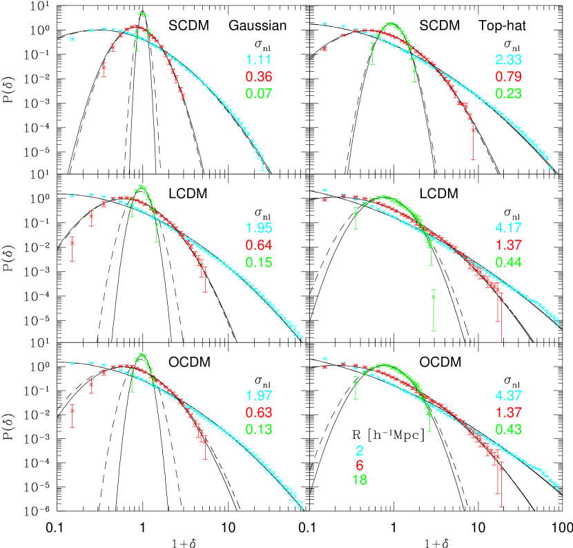
Figure 1: One-point PDFs in CDM models with Gaussian (left panels) and top-hat (right panels) smoothing windows; $R=2$$h^{-1}$Mpc(cyan), 6$h^{-1}$Mpc(red), and 18$h^{-1}$Mpc(green). The top, middle and bottom panels correspond to the PDFs in SCDM, LCDM, and OCDM. The solid and long-dashed lines represent the log-normal PDF adopting $\sigma_{\rm nl}$ calculated directly from the simulations and estimated from the nonlinear fitting formula of Peacock & Dodds (1996), respectively. The values of $\sigma_{\rm nl}$ in each panel are estimated from the simulations.

Consider first the one-point PDFs in CDM models (Fig. 1). The PDFs are constructed by binning the data with $\Delta\delta=0.1$, but we do not plot all the data points just for an illustrative purpose. We compute the density fields smoothed over Gaussian (Left panels) and Top-hat (Right panels) windows with different smoothing lengths;$R=2h^{-1}$Mpc, $6h^{-1}$Mpc and $18h^{-1}$Mpc plotted in cyan, red and green symbols with error-bars, respectively. The corresponding values of $\sigma_{\rm nl}$ are summarized in Table 2, and also shown on each panel. Solid lines show the log-normal PDFs adopting those $\sigma_{\rm nl}$ directly evaluated from simulations. The agreement between the log-normal model and the simulation results is quite impressive. A small deviation is noticeable only for $\delta\lower 2.15277pt\hbox{$\;\buildrel<\over{\sim}\;$}-0.5$.

We also show the log-normal PDFs in dashed lines, adopting $\sigma_{\rm nl}$ calculated from the nonlinear fitting formula of PD (values in parenthesis in Table 2). Therefore the predictions do not use the specific information of the current simulations, and are completely independent in this sense. While these predictions are in good agreement with simulation data for $R\lower 2.15277pt\hbox{$\;\buildrel<\over{\sim}\;$}6h^{-1}$Mpc, the results for $R=18h^{-1}$Mpc are rather different. Actually this discrepancy should be ascribed to the simulations themselves, not to the model predictions; Table 2 indicates that the $\sigma_{\rm nl}$ in the current simulations become systematically smaller than the PD predictions for larger $R$. This is because the simulations assume (incorrectly) no fluctuations beyond the scale of the simulation boxsize $L_{\rm box}$. This constraints systematically reduce the fluctuations as the smoothing scale $R$ approaches $L_{\rm box}$. We made sure that this is indeed the case by repeating the same analysis using the CDM simulations evolved in $L_{\rm box}=300h^{-1}{\rm Mpc}$ (Jing & Suto 1998); the variance of fluctuations at $R\leq 18h^{-1}$Mpc from the simulations agrees with the PD prediction within 2% accuracy. Thus we conclude that the log-normal PDF with the PD formula reproduces accurately the simulation results in the CDM models.

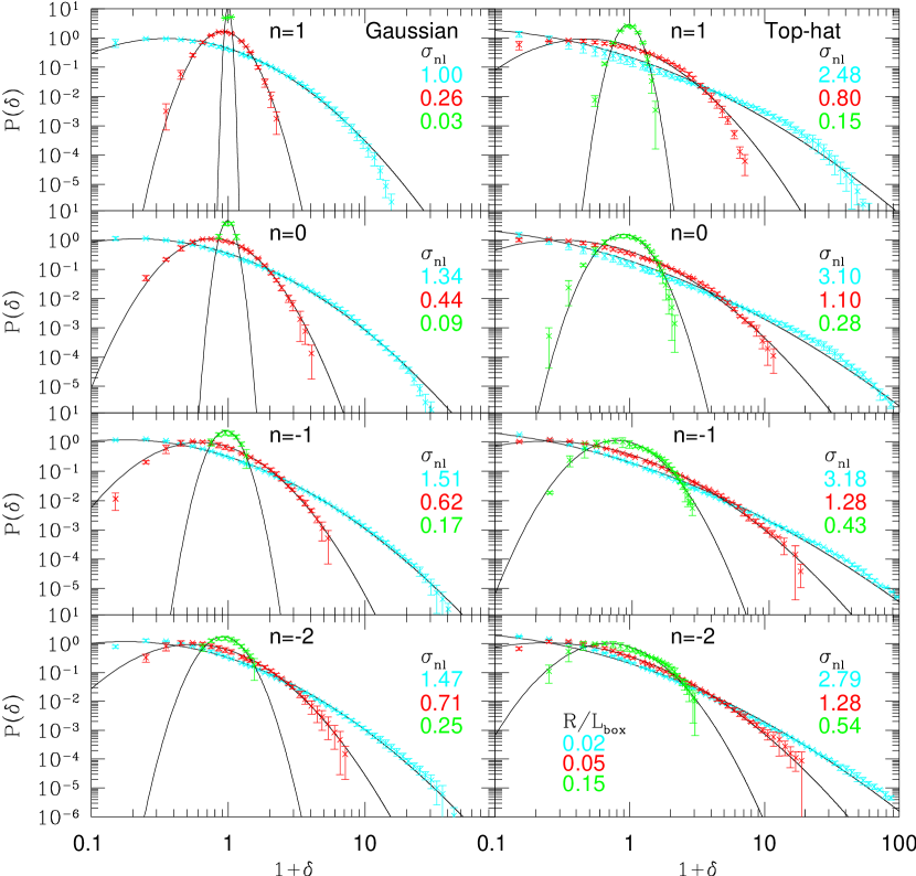
Figure 2: Same as Fig 1, but in the scale-free models ($n=1$ to $-2$ from top to bottom); $R=0.02L_{\rm box}$ (cyan), $0.05L_{\rm box}$ (red), and $0.15L_{\rm box}$ (green).

Next turn to the scale-free models. Figure 2 shows the similar plots corresponding to Figure 1 but for $n=1$ to $-2$ models (from top to bottom panels). In this figure, we compare the simulation data (symbols with error-bars) with the log-normal PDF predictions (solid lines) adopting $\sigma_{\rm nl}$ from simulations (Table 3). Generally their agreement is good also in these models. A closer look at Figure 2, however, reveals that the simulation results start to deviate from the log-normal predictions at both high and low density regions, and that the deviation seems to systematically increase as $n$ becomes larger. While this tendency is qualitatively consistent with the earlier claim by Bernardeau (1994) and Bernardeau & Kofman (1995) on the basis of the perturbation theory, our fully nonlinear simulations show that the deviation from the log-normal PDF is not so large even in these scale-free models.

To examine the validity of the log-normal PDF more quantitatively, we compare the normalized skewness $S\equiv\langle\delta^{3}\rangle/\langle\delta^{2}\rangle^{2}$ and the normalized kurtosis $K\equiv(\langle\delta^{4}\rangle-3\langle\delta^{2}\rangle^{2})/\langle\delta^{2}\rangle^{3}$. The log-normal PDF predicts that

$$S(R) = 3+\sigma_{\rm nl}^{2}(R),$$ (24)

$$K(R) = 16+15\sigma_{\rm nl}^{2}(R)+6\sigma_{\rm nl}^{4}(R)+\sigma_{\rm nl}^{6}(R),$$ (25)

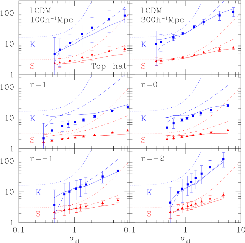
Figure 3: Normalized skewness $S$ and normalized kurtosis $K$ against $\sigma_{\rm nl}$ from simulations and the log-normal PDF predictions. The symbols represent the values estimated from simulations (the quoted $1\sigma$ error-bars represent the scatter in the realizations). The meaning of predictions plotted in different lines is explained in the text. Top-hat smoothing is assumed.

which are plotted in dotted lines in Figure3 for six models; two LCDM models with $L_{\rm box}=100h^{-1}$Mpc and $300h^{-1}$Mpc, and four scale-free models with $n=1$, 0, -1, and $-2$.

In practice, however, the density field $\delta$ in numerical simulations does not extend the entire range between $-1$ and $\infty$, but rather is limited as $\delta_{\rm min}<\delta<\delta_{\rm max}$ due to the finite size of the simulation box. Thus the $n$-th order moments of $\delta$ in simulations may be better related to

$$\langle\delta^{n}\rangle^{\prime}=\int_{\delta_{\rm min}}^{\delta_{\rm max}}\delta^{n}P_{\rm LN}^{(1)}(\delta)d\delta.$$ (26)

The specific values for $\delta_{\rm min}$ and $\delta_{\rm max}$ may be roughly estimated from the condition that the expectation number of independent sampling spheres in the simulation box for $\delta<\delta_{\rm min}$ or $\delta>\delta_{\rm max}$ becomes unity:

$$\frac{L_{\rm box}^{3}}{4\pi R^{3}/3}\int_{\delta_{\rm max}}^{\infty}P_{\rm LN}^{(1)}(\delta)d\delta = 1,$$ (27)

$$\frac{L_{\rm box}^{3}}{4\pi R^{3}/3}\int_{-1}^{\delta_{\rm min}}P_{\rm LN}^{(1)}(\delta)d\delta = 1.$$ (28)

Dashed lines in Figure 3 show the log-normal PDF predictions based on equations (26) to (28). The filled triangles and squares represent the measurement of $S$ and $K$ from the simulations, and finally the solid lines indicate the log-normal PDF predictions using equation (26) with the actual values for $\delta_{\rm min}$ and $\delta_{\rm max}$ in the simulations. Except for the $n=1$ scale-free model, the predictions in solid lines reproduce the simulation data very well, which indicates that the log-normal PDF is in fact a good approximation. The relatively large discrepancy between the log-normal prediction and the simulation in the $n=1$ model is real since one can clearly recognize the systematic tendency with respect to $n$; models with smaller $n$, i.e., with substantial power on large scales , are better described by the log-normal PDF. This is consistent with the discussion by Bernardeau (1994).

Incidentally both the current simulations and the log-normal PDF approximation confirmed the relatively strong scale-dependence of $S$ and $K$ for $\sigma_{\rm nl}>1$ as pointed out earlier by Lahav et al. (1993) and Suto (1993). In fact the degree of their scale-dependence is also sensitive to the underlying power spectrum. Thus the hierarchical ansatz for the higher-order clustering is not valid in general.

In summary, we find that the one-point log-normal PDF remains a fairly accurate model for the cosmological density distribution even up to $\sigma_{\rm nl}\sim 4$ and $\delta\sim 100$, fairly independently of the shape of the underlying power spectrum of density fluctuations. The range of validity turns out to be significantly broader than those from the previous studies based on lower-resolution simulations; $0.1\lower 2.15277pt\hbox{$\;\buildrel<\over{\sim}\;$}\sigma\lower 2.15277pt\hbox{$\;\buildrel<\over{\sim}\;$}0.6$ and $\delta\lower 2.15277pt\hbox{$\;\buildrel<\over{\sim}\;$}4$ (Kofman et al. 1994), and $0.3\lower 2.15277pt\hbox{$\;\buildrel<\over{\sim}\;$}\sigma\lower 2.15277pt\hbox{$\;\buildrel<\over{\sim}\;$}1.5$ and $\delta\lower 2.15277pt\hbox{$\;\buildrel<\over{\sim}\;$}9$ (Bernardeau & Kofman 1995), for instance.

3.3 The two-point PDF

While we would like to perform the similar comparison for the two-point PDFs, it is a function of four variables, $\delta_{1}$, $\delta_{2}$, $R$, and $r$, and thus the comparison becomes rather complicated. Therefore we decided to use the conditional two-point PDF for the purpose:

$$P^{(2)}(\delta_{1}|\delta_{2};r)\equiv\frac{P^{(2)}(\delta_{1},\delta_{2};r)}{P^{(1)}(\delta_{2})}.$$ (29)

Since we already made sure that the one-point PDF is very accurately approximated by the log-normal, our task is to see if simulation results fit the conditional two-point log-normal PDF:

$$P^{(2)}_{\rm LN}(\delta_{1}|\delta_{2};r)\equiv\sqrt{\frac{S}{2\pi(S^{2}-X^{2})}}\exp\left[-\frac{(SL_{1}-XL_{2})^{2}}{2S(S^{2}-X^{2})}\right]\frac{1}{(1+\delta_{1})}.$$ (30)

The evaluation of the conditional two-point PDFs from simulations is carried out as follows. From the smoothed density fields computed on the $512^{3}$ grid points, we first select those grid points with $\delta_{2}-\Delta\delta_{2}/2<\delta<\delta_{2}+\Delta\delta_{2}/2$. The bin size $\Delta\delta_{2}$ is adjusted for each value of $\delta_{2}$ so that approximately $10^{5}$ grid points satisfy the condition. Next we pick up all grid points separated at $r-\Delta r/2\sim r+\Delta r/2$ from the above grids. The separation interval $\Delta r$ is chosen so that $4\pi r^{2}\Delta r(512/L_{\rm box})^{3}\sim 10^{3}$. Finally we compute the conditional two-point PDF with a constant bin size of 0.1 in $\delta_{1}$.

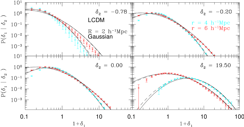
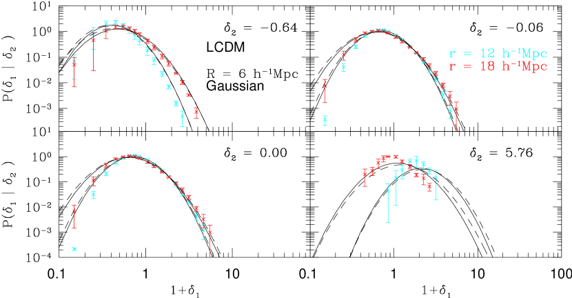
Figure 4: Two-point PDFs in LCDM model with Gaussian smoothing over $R=2$$h^{-1}$Mpc(upper four panels) and $R=6$$h^{-1}$Mpc(lower four panels). The results at separation $r=2R$ and $3R$ are plotted. The solid and long-dashed lines represent the log-normal PDF adopting $\sigma_{\rm nl}$ and $\xi_{\rm nl}$ calculated directly from the simulations and estimated from the nonlinear fitting formula of Peacock & Dodds (1996), respectively.

Figure 4 plots the resulting PDFs for the LCDM model with the Gaussian smoothing window; the upper four panels show the PDFs for the separation $r=4$ and $6h^{-1}{\rm Mpc}$ and the smoothing length $R=2h^{-1}{\rm Mpc}$, while the lower four panels for $r=12$ and $18h^{-1}{\rm Mpc}$ and $R=6h^{-1}{\rm Mpc}$. Solid lines indicate the conditional log-normal PDFs adopting the values of $\sigma_{\rm nl}$ and $\xi_{\rm nl}$ from simulations, while dashed lines show those using the PD predictions (Tables 2 to 5). Clearly the log-normal PDF is a reasonably good approximation. The deviation at $\delta_{2}\lower 2.15277pt\hbox{$\;\buildrel<\over{\sim}\;$}-0.5$, on the other hand, seems real and may be an enhanced feature that we noted in the one-point PDF (Fig. 1).

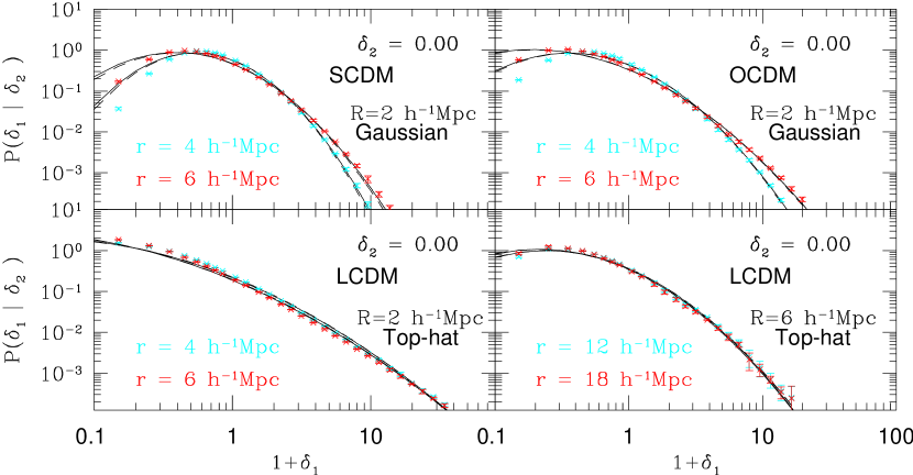
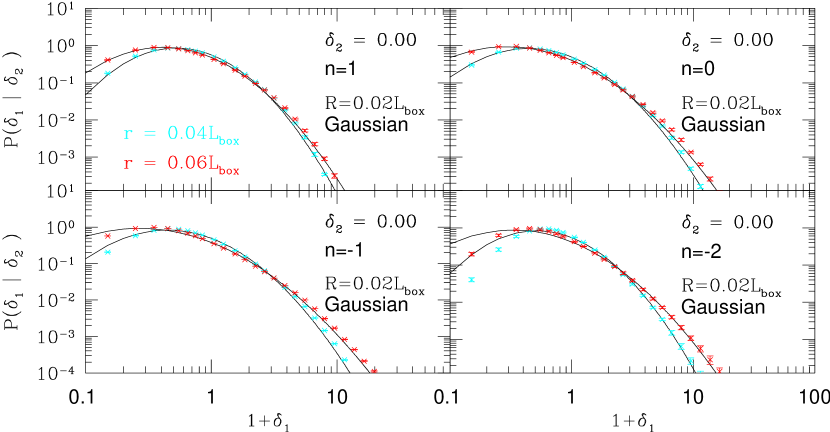
Figure 5: Two-point PDFs for different models and smoothing window functions. The upper four panels plot the results in CDM models, while the lower four panels in scale-free models.

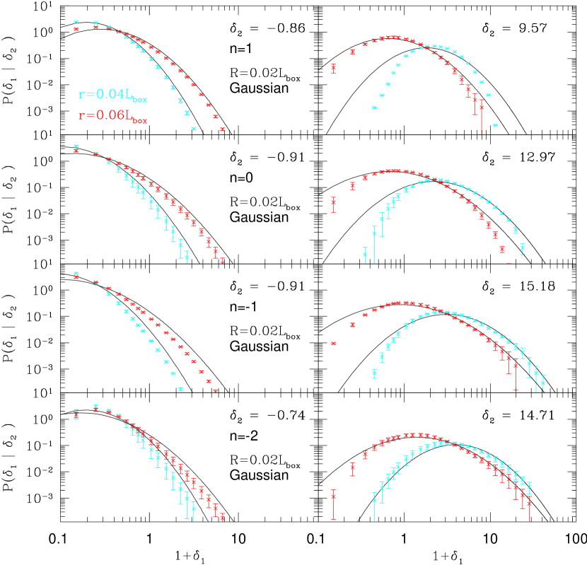
Figure 6: Two-point PDFs for the scale-free models at negative (left) and positive (right) tails of the distribution of $\delta_{2}$.

Figure 5 indicates that the good agreement is achieved not only in the Gaussian smoothed LCDM model, but also can be found in the other models and/or the top-hat smoothing. Figure 6 plots the conditional two-point PDFs at $\delta_{2}\lower 2.15277pt\hbox{$\;\buildrel<\over{\sim}\;$}-0.7$ and $\delta_{2}\lower 2.15277pt\hbox{$\;\buildrel>\over{\sim}\;$}10$ in the scale-free models, where the deviation from the log-normal becomes manifest. Considering the error-bars estimated from the different realizations for each model, the deviation seems statistically real.

As in the case of the one-point PDF, we illustrate the validity of the two-point log-normal PDF using the moments. Specifically we evaluate $\langle(\delta_{1}\delta_{2})^{2}\rangle$ and $\langle(\delta_{1}\delta_{2})^{3}\rangle$ according to

$$\langle(\delta_{1}\delta_{2})^{n}\rangle(r)\equiv{\int\!\!\!\!\int}_{{\cal C}(\delta_{1},\delta_{2})}(\delta_{1}\delta_{2})^{n}P_{\rm LN}^{(2)}(\delta_{1},\delta_{2};r)d\delta_{1}d\delta_{2},$$ (31)

where we select the range of the integration as

$${\cal C}(\delta_{1},\delta_{2})=\{(\delta_{1},\delta_{2})|\delta_{\rm min}\leq\delta_{1}\leq\delta_{\rm max},\delta_{\rm min}\leq\delta_{2}\leq\delta_{\rm max}\},$$ (32)

from the values of $\delta_{\rm min}$ and $\delta_{\rm max}$ directly measured from each simulation model. The results are summarized in Table 6, which indicates again that the two-point log-normal PDF predictions reproduce the simulation data except for $n\geq 0$. Thus we also conclude that the two-point log-normal model describes fairly well the PDF of cosmological fluctuations for most regions of $\delta_{1}$ and $\delta_{2}$ of interest; the small but finite deviations exist only in $\delta_{1}\lower 2.15277pt\hbox{$\;\buildrel<\over{\sim}\;$}-0.5$ and/or $\delta_{2}\lower 2.15277pt\hbox{$\;\buildrel<\over{\sim}\;$}-0.5$, and in $\delta_{1}\lower 2.15277pt\hbox{$\;\buildrel>\over{\sim}\;$}10$ and $\delta_{2}\lower 2.15277pt\hbox{$\;\buildrel>\over{\sim}\;$}10$.

3.4 Does the log-normal transformation approximate the gravitational evolution of the density fluctuations ?

The agreement between the log-normal predictions and the simulation results might be interpreted as indirect evidence that the log-normal transformation (eq.[8]) is a good approximation for the nonlinear gravitational growth of the cosmological density fluctuations, at least on average.

In order to see if this is really the case, we consider the relation of the smoothed density fields at the same comoving position but at different redshifts $z_{1}$ and $z_{2}$. For this purpose, we use one realization from the LCDM model evolved in $L_{\rm box}=300{\hbox{$h^{-1}$}{\rm Mpc}}$. If the log-normal transformation (8) is exact, the density fluctuations, $\delta(z_{1})$ and $\delta(z_{2})$, should satisfy

$$1+\delta(z_{2})=\frac{1}{\sqrt{1+\sigma^{2}_{\rm nl}(z_{2})}}\exp\left[\frac{\sqrt{\ln\{1+\sigma^{2}_{\rm nl}(z_{2})\}}}{\sqrt{\ln\{1+\sigma^{2}_{\rm nl}(z_{1})\}}}\ln\left\{\sqrt{1+\sigma^{2}_{\rm nl}(z_{1})}(1+\delta(z_{1}))\right\}\right].$$ (33)

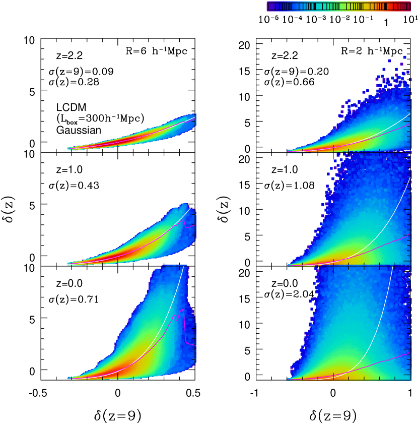
Figure 7: Contour plots of the joint probability $P(\delta(z)~{}|~{}\delta(z=9))$ in the LCDM model ($L_{\rm box}=300{\hbox{$h^{-1}$}{\rm Mpc}}$) with Gaussian smoothing window; $R=6h^{-1}$Mpc (right) and $R=2h^{-1}$Mpc (right). The top, middle and bottom panels correspond to correlations of $\delta(z=2.2)$, $\delta(z=1)$, and $\delta(z=0)$ against $\delta(z=9)$, respectively. The white lines represent the log-normal transformation (33) and the magenta lines are the conditional mean at a fixed $\delta(z=9)$.

Figure 7 plots the color contour of the joint probability $P(\delta(z),\delta(z=9))$ of densities at $z=2.2$, $1.0$, and $0$ against that at $z=9$ on the same grid points in the LCDM model. We adopt the Gaussian smoothing with $R=6h^{-1}{\rm Mpc}$ (Left) and $2h^{-1}{\rm Mpc}$ (Right). The solid lines in white and magenta represent the the log-normal transformation (33) and the conditional mean from simulations for a fixed $\delta(z=9)$. The log-normal transformation traces the mean relation of simulations to some extent only when the nonlinearity is weak (see, higher $z$ and larger $R$ cases). On the other hand, in the nonlinear region, the transformation (33) starts to deviate from the mean relation of the simulations significantly, and the distribution around the mean relation becomes broad. The similar tendency was found in a somewhat different analysis by Coles, Melott, & Shandarin (1993). In a sense this is a physically natural and expected result, but then it makes even more difficult to account for the good agreement between the log-normal and simulation PDFs in those scales.

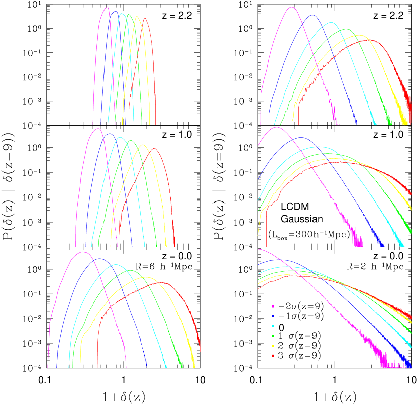
Figure 8: Conditional probability $P(\delta(z)~{}|~{}\delta(z=9))$ for a fixed $\delta(z=9)$ corresponding to each panel of Fig. 7. In each panel, results for $\delta(z=9)=-2$, $-1$, 0, 1, 2, and 3 times the $\sigma(z=9)$, the rms of $\delta(z=9)$, are plotted.

To better understand the distribution of the linear and its evolved density fields, we compute the conditional probability $P(\delta(z)~{}|~{}\delta(z=9))$, i.e., the slice of Figure 7 at a given $\delta(z=9)$. The results are plotted in Figure 8 which exhibits a some regularity in the distribution. The peak positions seem to show some scaling with respect to the value of $\delta(z=9)$, and also the tail of the distribution asymptotically approaches a single power-law. While we do not yet fully understand the behavior, this regularity in the distribution function may be useful in explaining our findings that the one-point and two-point log-normal PDFs work well empirically.

4 CONCLUSIONS AND DISCUSSION

In the present paper, we have estimated the probability distribution functions of cosmological density fluctuations from the high-resolution N-body simulations with the Gaussian initial condition. In particular, we have critically examined the validity of the log-normal models for the one- and two-point PDFs both in weakly and in strongly nonlinear regimes.

We have shown that the one-point log-normal PDF is a fairly accurate model not only in a weakly nonlinear regimes as claimed previously, but also in more strongly nonlinear regimes even up to $\sigma_{\rm nl}\sim 4$ and $\delta\sim 100$. Furthermore, we extended the analysis to the two-point PDF, and found that the log-normal PDF serves also as an empirically accurate model for the range of densities of interest. This is the case fairly independently of the shape of the underlying power spectrum of density fluctuations, although models with large power on small scales (e.g., $n\geq 0$ scale-free models in our examples) seem to show a small deviation from the log-normal prediction at the tails of the distribution, especially for $\delta\lower 2.15277pt\hbox{$\;\buildrel<\over{\sim}\;$}-0.5$. In particular, the log-normal PDF reproduces very well the skewness and kurtosis measured from the simulation data, when the finite size of the simulation volume is properly taken into account.

The degree of agreement of the log-normal models that we have shown is amazing considering the fact that the underlying mapping between the initial and the evolved density fields differs significantly from the simulation results even in an averaged sense. We have explicitly shown the probability distribution of the initial and the evolved density fields from simulations, although we were not able to provide a physical explanation for the origin of the log-normal PDF. This should be left as our future work and we would like to come back later elsewhere. For this purpose, other theoretical approaches based on perturbation theory (Bernardeau 1992, 1994) and the spherical collapse model (Fosalba & Gaztañaga 1998) may be helpful.

Nevertheless our present work provides an empirical justification for the use of the log-normal PDF in a variety of theoretical model predictions. For instance, Matsubara & Yokoyama (1996) proposed to evaluate the effect of the nonlinear gravitational evolution on the genus statistics using the log-normal mapping. Taruya & Suto (2000) constructed an analytical model for halo biasing on the basis of the one-point log-normal PDF of underlying mass density field. Hikage, Taruya, & Suto (2001) applied this biasing model in their predictions of the genus for clusters of galaxies.

Finally, the present results might be useful in considering the prediction of weak lensing statistics (Valageas 2000; Munshi & Jain 2000). To construct a model for PDF in redshift space is another important topic (e.g., Watts & Taylor 2001; Hui, Kofman & Shandarin 2000), which is relevant in discussing Ly-$\alpha$ forests (Gaztañaga & Croft 1999).

We thank Y. P. Jing for kindly providing us his N-body data, and an anonymous referee for constructive comments. I.K. and A.T. gratefully acknowledge support from Takenaka-Ikueikai fellowship, and a JSPS (Japan Society for the Promotion of Science) fellowship, respectively. Numerical computations were carried out at RESCEU (Research Center for the Early Universe, University of Tokyo), ADAC (the Astronomical Data Analysis Center) of the National Astronomical Observatory, Japan, and at KEK (High Energy Accelerator Research Organization, Japan). This research was supported in part by the Grant-in-Aid by the Ministry of Education, Science, Sports and Culture of Japan (07CE2002, 12640231) and by the Supercomputer Project (No.00-63) of KEK.

Table 1: Simulation parameters for the CDM models.

Model	$\Omega_{0}$	$\lambda_{0}$	$\Gamma$	$\sigma_{8}$	$L_{\rm box}$[$h^{-1}$Mpc]	realizations
SCDM	1.0	0.0	0.50	0.6	100	3
LCDM	0.3	0.7	0.21	1.0	100	3
LCDM300	0.3	0.7	0.21	1.0	300	3
OCDM	0.3	0.0	0.25	1.0	100	3

Table 2: Amplitude of $\sigma_{\rm nl}(R)$ evaluated from the CDM simulations. The values in parenthesis denote those estimated from the nonlinear fitting formula of Peacock & Dodds (1996).

smoothing	$R$ [$h^{-1}$Mpc]	SCDM	LCDM	OCDM
	2	2.33 (2.24)	4.17 (4.08)	4.37 (4.23)
top-hat	6	0.79 (0.77)	1.37 (1.40)	1.37 (1.38)
	18	0.23 (0.24)	0.44 (0.50)	0.43 (0.47)
	2	1.11 (1.08)	1.95 (1.96)	1.97 (1.96)
Gaussian	6	0.36 (0.35)	0.64 (0.69)	0.63 (0.67)
	18	0.065 (0.090)	0.15 (0.22)	0.13 (0.21)

Table 3: Rms $\sigma_{\rm nl}(R)$ in the scale-free simulations.

smoothing	$R$ [$L_{\rm box}$]	$n=1$	$n=0$	$n=-1$	$n=-2$
	0.02	2.48	3.10	3.18	2.79
top-hat	0.05	0.80	1.10	1.28	1.28
	0.15	0.15	0.28	0.43	0.54
	0.02	1.00	1.34	1.51	1.47
Gaussian	0.05	0.26	0.44	0.62	0.71
	0.15	0.03	0.09	0.17	0.25

Table 4: Amplitude of $\xi_{\rm nl}(r;R)$ evaluated from the CDM simulations with Gaussian smoothing. The values in parenthesis denote those estimated from the nonlinear fitting formula of Peacock & Dodds (1996).

$R$ [$h^{-1}$Mpc]	$r$ [$h^{-1}$Mpc]	SCDM	LCDM	OCDM
2	4	0.68 (0.64)	2.15 (2.10)	2.05 (2.06)
2	6	0.36 (0.35)	1.10 (1.15)	1.06 (1.10)
6	12	0.058 (0.063)	0.21 (0.26)	0.20 (0.24)
6	18	0.021 (0.028)	0.10 (0.144)	0.087 (0.127)

Table 5: Two-point correlation $\xi_{\rm nl}(r;R)$ in the scale-free simulations with Gaussian smoothing.

$R$ [$L_{\rm box}$]	$r$ [$L_{\rm box}$]	$n=1$	$n=0$	$n=-1$	$n=-2$
0.02	0.04	0.40	0.82	1.29	1.35
0.02	0.06	0.13	0.36	0.67	0.83

Table 6: Two-point moments, $\langle(\delta_{1}\delta_{2})^{2}\rangle$ and $\langle(\delta_{1}\delta_{2})^{3}\rangle$, from simulations and the log-normal PDF predictions. The LCDM models adopt the Gaussian smoothing with $R=2{\hbox{$h^{-1}$}{\rm Mpc}}$ and the moments are evaluated at the pair-separation of $r=4{\hbox{$h^{-1}$}{\rm Mpc}}$. For the scale-free models, $R=0.02L_{\rm box}$ and $r=0.04L_{\rm box}$.

Model	$\langle(\delta_{1}\delta_{2})^{2}\rangle$	$\langle(\delta_{1}\delta_{2})^{3}\rangle$	$\delta_{\rm min}$	$\delta_{\rm max}$
LCDM	$(0.76\pm 0.4)\times 10^{3}$	$(1.5\pm 1.4)\times 10^{6}$	$\cdots$	$\cdots$
log-normal	$0.64\times 10^{3}$	$1.1\times 10^{6}$	$-0.96$	90
LCDM300	$(1.4\pm 0.2)\times 10^{3}$	$(4.9\pm 1.5)\times 10^{6}$	$\cdots$	$\cdots$
log-normal	$1.3\times 10^{3}$	$6.2\times 10^{6}$	$-0.98$	165
$n=1$	$3.1\pm 0.1$	$73\pm 11$	$\cdots$	$\cdots$
log-normal	4.0	140	$-0.98$	14
$n=0$	$24\pm 3$	$(2.6\pm 0.6)\times 10^{3}$	$\cdots$	$\cdots$
log-normal	30	$5.6\times 10^{3}$	$-0.99$	30
$n=-1$	$88\pm 18$	$(2.2\pm 1.0)\times 10^{4}$	$\cdots$	$\cdots$
log-normal	102	$3.9\times 10^{4}$	$-0.98$	42
$n=-2$	$120\pm 40$	$(4.1\pm 2.1)\times 10^{4}$	$\cdots$	$\cdots$
log-normal	120	$5.3\times 10^{4}$	$-0.96$	46

References

- Bardeen et al. (1986) Bardeen,J.M., Bond,J.R., Kaiser,N., & Szalay,A.S. 1986, ApJ, 304, 15
- Bernardeau (1992) Bernardeau, F. 1992, ApJ, 392, 1
- Bernardeau (1994) Bernardeau, F. 1994, A&A, 291, 697
- Bernardeau (1996) Bernardeau, F. 1996, A&A, 312, 11
- Bernardeau & Kofman (1995) Bernardeau, F. & Kofman, L. 1995, ApJ, 443, 479
- Bouchet et al. (1993) Bouchet, F., Strauss, M. A., Davis, M., Fisher, K. B., Yahil, A., & Huchra, J. P. 1993, ApJ, 417, 36
- Coles & Jones (1991) Coles, P., & Jones, B. 1991, MNRAS, 248, 1
- Coles, Melott, & Shandarin (1993) Coles, P., Melott, A. L., & Shandarin, S. F. 1993, MNRAS, 260, 765
- Colombi, Bouchet, & Schaeffer (1995) Colombi, S., Bouchet, F. R., & Schaeffer, R. 1995, ApJS, 96, 401
- Fosalba & Gaztanaga (1998) Fosalba, P., & Gaztañaga, E. 1998, MNRAS, 301, 503
- Gaztañaga & Croft (1999) Gaztañaga, E., & Croft, R. A. C. 1999, MNRAS, 309, 885
- Gaztañaga & Yokoyama (1993) Gaztañaga, E., & Yokoyama, J. 1993, ApJ, 403, 450
- Hamilton (1985) Hamilton, A. J. S. 1985, ApJ, 292, L35
- Hikage, Taruya, & Suto (2001) Hikage, C., Taruya, A., & Suto, Y. 2001, ApJ, 556, August 1st issue, in press
- Hubble (1934) Hubble, E. P. 1934, ApJ, 79, 8
- Hui, Kofman & Shandarin (2000) Hui, L., Kofman, L., & Shandarin, S. 2000, ApJ, 537, 12
- Jing (1998) Jing, Y. P. 1998, ApJ, 503, L9
- Jing & Suto (1998) Jing, Y. P., & Suto, Y. 1998, ApJ, 494, L5
- Kitayama & Suto (1997) Kitayama, T., & Suto, Y. 1997, ApJ, 490, 557
- Kofman et al. (1994) Kofman, L., Bertschinger, E., Gelb, J. M., Nusser, A., & Dekel, A. 1994, ApJ, 420, 44
- Lahav et al. (1993) Lahav, O., Itoh, M., Inagaki, S., & Suto, Y. 1993, ApJ, 402, 387
- Matsubara & Yokoyama (1996) Matsubara, T., & Yokoyama, J. 1996, ApJ, 463, 409
- Munshi & Jain (2000) Munshi, D., & Jain, B. 2000, MNRAS, 318, 109
- Peacock & Dodds (1996) Peacock, J. A., & Dodds, S. J. 1996, MNRAS, 280, L19 (PD)
- Saslaw (1985) Saslaw, W.C. 1985, Gravitational Physics of Stellar and Galactic Systems, (Cambridge: Cambridge University Press)
- Suginohara & Suto (1991) Suginohara, T., & Suto, Y. 1991, PASJ, 43, L17
- Suto, Itoh & Inagaki (1990) Suto, Y., Itoh, M., & Inagaki, S. 1990, ApJ, 350, 492
- Suto (1993) Suto, Y. 1993, Prog.Theor.Phys., 90, 1173
- Szapudi & Colombi (1996) Szapudi, I., & Colombi, S. 1996, ApJ, 470, 131
- Taruya & Suto (2000) Taruya, A., & Suto, Y. 2000, ApJ, 542, 559
- Taylor & Watts (2000) Taylor, A. N., & Watts, P. I. R. 2000, MNRAS, 314, 92
- Ueda & Yokoyama (1996) Ueda, H., & Yokoyama, J. 1996, MNRAS, 280, 754
- Valageas (2000) Valageas, P. 2000, A&A, 356, 771
- Watts & Taylor (2001) Watts, P. I. R., & Taylor, A. N. 2001, MNRAS, 320, 139