Oxygen line formation in late-F through early-K disk/halo stars

In order to investigate the formation of O i 7771–5 and [O i] 6300/6363 lines, extensive non-LTE calculations for neutral atomic oxygen were carried out for wide ranges of model atmosphere parameters, which are applicable to early-K through late-F halo/disk stars of various evolutionary stages.

The formation of the triplet O i lines was found to be well described by the classical two-level-atom scattering model, and the non-LTE correction is practically determined by the parameters of the line-transition itself without any significant relevance to the details of the oxygen atomic model. This simplifies the problem in the sense that the non-LTE abundance correction is essentially determined only by the line-strength ($W_{\lambda}$), if the atmospheric parameters of $T_{\rm eff}$, $\log g$, and $\xi$ are given, without any explicit dependence of the metallicity; thus allowing a useful analytical formula with tabulated numerical coefficients. On the other hand, our calculations lead to the robust conclusion that LTE is totally valid for the forbidden [O i] lines.

An extensive reanalysis of published equivalent-width data of O i 7771–5 and [O i] 6300/6363 taken from various literature resulted in the conclusion that, while a reasonable consistency of O i and [O i] abundances was observed for disk stars ($-1\la[{\rm Fe}/{\rm H}]\la 0$), the existence of a systematic abundance discrepancy was confirmed between O i and [O i] lines in conspicuously metal-poor halo stars ($-3\la[{\rm Fe}/{\rm H}]\la-1$) without being removed by our non-LTE corrections, i.e., the former being larger by $\sim 0.3$ dex at $-3\la[{\rm Fe}/{\rm H}]\la-2$.

An inspection of the parameter-dependence of this discordance indicates that the extent of the discrepancy tends to be comparatively lessened for higher $T_{\rm eff}/\log g$ stars, suggesting the preference of dwarf (or subgiant) stars for studying the oxygen abundances of metal-poor stars.

1 Introduction

Oxygen abundance determination in F–K stars is one of the most controversial and interesting topics in stellar spectroscopy, especially concerning the behavior of the [O/Fe] ratio in metal-poor halo stars (see, e.g., Carretta et al. 2000; King 2000; Israelian et al. 2001; Nissen et al. 2002; and the references therein).

Namely, we are faced with a problem currently in hot controversy on the observational side, which stems from the fact that each of the different groups of spectral lines, (a) high-excitation permitted O i lines (e.g., 7773 triplet), (b) low-excitation forbidden [O i] lines (6300/6363 lines), and (c) OH lines at UV ($\sim$ 3100–3200 $\rm\AA$), do not necessarily yield reasonably consistent oxygen abundances in metal-poor stars.

More precisely, a distinct discrepancy is occasionally reported between the abundances derived from O i and [O i] lines in the sense that the former tend to yield systematically higher oxygen abundances than the latter in metal-poor stars (see, e.g., Cavallo et al. 1997), in contrast to the relation between O i and OH lines which give more or less consistent abundances (e.g., Boesgaard et al. 1999). As a result, different trends of O-to-Fe ratio, an important tracer of early nucleosynthesis in our Galaxy, have naturally been suggested: (1) plateau-like [O/Fe] from [O i] lines, and (2) ever-rising [O/Fe] from O i or OH lines.

Admittedly, what has been described above is nothing but a rough summary and the actual situation is more complicated than such a simple dichotomic picture. For example, the O i vs. [O i] discordance appears to be observed only in metal-poor halo stars, since such a systematic disagreement is absent in population I G–K giants (cf. Takeda et al. 1998). Moreover, according to Carretta et al.’s (2000) recent investigation of very metal-poor stars (mainly giants), a “nearly flat” [O/Fe] trend was concluded consistently from both of the O i and [O i] lines. Very recently, on the other hand, Nissen et al. (2002) also obtained nearly consistent O i and [O i] abundances of metal-poor dwarfs and subgiants, but at a “quasi-linearly increasing” trend in contrast to Carretta et al. (2000), though an application of the 3D hydrodynamical model atmospheres (taking into account the atmospheric granular motions) tends to deteriorates the agreement.

This confusion makes us wonder which on earth is the correct and reliable indicator of the oxygen abundance. Generally speaking, a modest view currently preferred by many people is that [O i] lines are less problematic and more creditable due to their weak $T_{\rm eff}$-sensitivity as well as the general belief of the validity for the assumption of LTE, while O i and OH lines are less reliable because of the uncertainties involved with the non-LTE correction (O i) or with the 3D effect of atmospheric inhomogeneity (OH).

Recently, however, we cast doubt on this conservative picture and suggested the possibility of erroneously underestimated abundances from [O i] lines (i.e., the problem may be due to the formation of forbidden lines rather than that of permitted lines) based on our analysis of seven metal-poor stars (Takeda et al. 2000), which indicated the tendency of above-mentioned O i vs. [O i] discrepancy (though a small number of sample stars prevented us from making any convincing argument).

Motivated by that work suggesting the necessity of a follow-up study to check if our hypothesis is reasonable or not, we decided to revisit this O i vs. [O i] problem while paying special attention to the topic of the non-LTE correction to be applied, one of the controversial factors in oxygen abundance determination. Toward this aim, we carried out new extensive non-LTE calculations, based on which the numerous published equivalent-width data were reanalyzed to derive the non-LTE abundances, in order to discuss whether or not the abundance discrepancy between O i and [O i] really exists, which we hope to shed some light on the oxygen problem of metal-deficient stars mentioned above.

This paper is organized as follows:
— First, extensive tables of non-LTE corrections for the O i 7771–5 triplet lines over a wide range of atmospheric parameters are presented, so that they may be applied to late-F through early-K dwarfs/giants of various metallicities.
— Second, in order for application of such tables to actual analysis of observational data, we try to find out a useful analytical formula for evaluating non-LTE corrections of these O i triplet lines for any given atmospheric parameters ($T_{\rm eff}$, $\log g$, $\xi$) and an observed equivalent width ($W_{\lambda}$).
— Third, we investigate the possibility of a non-LTE effect for the low-excitation forbidden [O i] 6300/6363 lines, for which few such attempt has ever been made.
— Fourth, equivalent-width data of O i 7771–5 lines as well as [O i] 6300/6363 lines taken from various literature are reanalyzed within the framework of the consistent system of analysis along with application of our non-LTE correction formula, in order to discuss the characteristics of [O/Fe] vs. [Fe/H] relation derived from permitted O i lines and forbidden [O i] lines separately.

Also, as a supplementary subject related to this study, the influence of the treatment of H i collision on the non-LTE corrections of O i 7771–5 lines was quantitatively estimated, and the consistency of the present choice of this parameter was checked by comparing the abundances of nearby solar-type stars derived from O i 7771–5, O i 6158, and [O i] 6300 lines. In addition, we also tried to qualitatively explain the line formation of O i 7771–5 in terms of the simple classical two-level-atom model, which gives us an insight to understanding the behavior of the non-LTE correction for these triplet lines. These are separately described in Appendices A and B, respectively.

2 Statistical equilibrium calculations

2.1 Atomic model

The procedures of our non-LTE calculations for neutral atomic oxygen are almost the same as those described in Takeda (1992), which should be consulted for details. We only mention here that the calculation of collision rates in rate equations basically follows the recipe described in Takeda (1991). Especially, the effect of H i collisions, an important key factor in the non-LTE calculation of F–K stars, was treated according to Steenbock & Holweger’s (1984) classical formula without any correction as has been done in our oxygen-related works so far, which we believe to be a reasonable choice as far as our calculations are concerned (cf. Takeda 1995, and Appendix A).

There is, however, an important change concerning the atomic model as described below. The model oxygen atom adopted in Takeda (1992) was constructed mainly based on the atomic data (energy level data and $gf$ values) compiled by Kurucz & Peytremann (1972), with $\sim$ 30 additional radiative transitions which were missing in their compilation [e.g., resonance transitions whose transition probabilities were taken from Morton (1991)]. This old model did not include the 2s² 2p^{4 3}P–2p^4 1D transition (corresponding to [O i] 6300/6363 lines) explicitly as the radiative transition (i.e., it was treated as if being completely radiatively forbidden in spite of its actually weak connection), simply because it was not contained in Kurucz & Peytremann (1972). We also noticed that several important UV radiative transitions originating upward from the 2p^4 1D term (i.e., upper term of [O i] 6300/6363) were also missing in that old model atom for the same reason.

We, therefore, newly reconstructed the model oxygen atom exclusively based on the data of Kurucz & Bell (1995), with additional transition probability data for 2p^4 1D–3s ³S^o and 2p^4 1D–3s ⁵S^o transitions taken from Vienna Atomic Line Database (VALD; Kupka et al. 1999). Regarding the collisional rate $C_{1-2}$ for the [O i] transition (2s² 2p^{4 3}P–2p^4 1D) mentioned above, the cross-section given in Osterbrock (1974) were used for evaluating the electron collision rates ($C_{1-2}^{\rm e}$), and the H i collision rates ($C_{1-2}^{\rm H}$) were estimated by scaling $C_{1-2}^{\rm e}$ (cf. Takeda 1991). The resulting atomic model comprises 87 terms (including terms up to 3p^′′ 1S, 6d^′ 3P, 10d ⁵D for the singlet, triplet, and quintet system, respectively) and 277 radiative transitions, which is similar to the old one in terms of the complexity but must be significantly improved, especially for studying the formation of [O i] lines (i.e., more realistic treatment of the 1–2 interaction and the inclusion of as many UV transitions connecting to the upper term 2 as possible).

Given the changes explained above, the reader can find the description on the adopted rates in the statistical-equilibrium calculation in Sect. 2.1 of Takeda (1992). Some additional details (which were not explicitly described therein) are given below:
— The population of neutral hydrogen (necessary for computing the rates of H i collision or the charge-exchange reaction) was taken from the model atmospheres (i.e., LTE ionization equilibrium).
— For the upper terms other than the lowest 8 terms mentioned in Sect. 2.1 of Takeda (1992), the hydrogenic approximation was used for the photoionization cross section.
— The photoionizing radiation field was computed based on Kurucz’s (1993a) ATLAS9 model atmospheres while incorporating the line opacity with the help of Kurucz’s (1993b) opacity distribution function.
— The collisional rates for those transitions, which are not explicitly mentioned in Sect. 2.1 of Takeda (1992), were evaluated according to the procedure described in Sect. 3.1.3 of Takeda (1991).

2.2 Model atmospheres

We planned to make our calculations applicable to stars from near-solar metallicity (population I) down to very low metallicity (extreme population II) at late-F through early-K spectral types in various evolutionary stages (i.e., dwarfs, subgiants, giants, and supergiants). We, therefore, decided to carry out non-LTE calculations on the extensive grid of one hundred ($5\times 5\times 4$) model atmospheres resulting from combinations of five $T_{\rm eff}$ values (4500, 5000, 5500, 6000, 6500 K), five $\log g$ (cm s^-2) values (1.0, 2.0, 3.0, 4.0, 5.0), and four metallicities (represented by [Fe/H]) (0.0, $-1.0$, $-2.0$, $-3.0$). As for the stellar model atmospheres, we adopted Kurucz’s (1993a) ATLAS9 models corresponding to the microturbulent velocity ($\xi$) of 2 ${\rm km\>s^{-1}}$.

2.3 Oxygen abundance and microturbulence

Regarding the oxygen abundance used as an input value in non-LTE calculations, we assumed $\log\epsilon_{\rm O}^{\rm input}$ = 8.93 + [Fe/H] +[O/Fe], where [O/Fe] = 0.0 for the solar metallicity models ([Fe/H] = 0) and [O/Fe] = +0.5 for the other metal-deficient models ([Fe/H] = $-1$, $-2$, and $-3$). Namely, the solar oxygen abundance of 8.93 taken from Anders & Grevesse (1989), which is also the canonical value used in the ATLAS9 models, was adopted for the normal-metal models, while the metallicity-scaled oxygen abundance plus 0.5 dex (allowing for the characteristics of $\alpha$ element) was assigned to the metal-poor models.

The microturbulent velocity (appearing in the line-opacity calculations along with the abundance) was assumed to be 2 ${\rm km\>s^{-1}}$, to make it consistent with the model atmosphere.

3 Non-LTE corrections

3.1 Evaluation procedures

Here, we describe how the non-LTE abundance corrections are evaluated after the departure coefficients, $b\equiv n_{\rm NLTE}/n_{\rm LTE}^{*}$, have been established by statistical equilibrium calculations.

For an appropriately assigned oxygen abundance ($A^{\rm a}$) and microturbulence ($\xi^{\rm a}$), we first calculated the non-LTE equivalent width ($W^{\rm NLTE}$) of the line by using the computed non-LTE departure coefficients ($b$) for each model atmosphere. Next, the LTE ($A^{\rm L}$) and NLTE ($A^{\rm N}$) abundances were computed from this $W^{\rm NLTE}$ while regarding it as if being a given observed equivalent width. We can then obtain the non-LTE abundance correction, $\Delta$, which is defined in terms of these two abundances as $\Delta\equiv A^{\rm N}-A^{\rm L}$.

Strictly speaking, the departure coefficients [$b(\tau)$] for a model atmosphere correspond to the oxygen abundance and the microturbulence of $\log\epsilon_{\rm O}^{\rm input}$ and 2 ${\rm km\>s^{-1}}$ adopted in the calculations (cf. Sect. 2.3). Nevertheless, considering the fact that the departure coefficients (i.e., ratios of NLTE to LTE number populations) are (unlike the population itself) not much sensitive to small changes in atmospheric parameters, we applied such computed $b$ values also to evaluating $\Delta$ for slightly different $A^{\rm a}$ and $\xi^{\rm a}$ from those fiducial values assumed in the statistical equilibrium calculations. Hence, we evaluated $\Delta$ for three $A^{\rm a}$ values ($\log\epsilon_{\rm O}^{\rm input}$ and $\pm 0.3$ dex perturbation) as well as three $\xi$ values (2 ${\rm km\>s^{-1}}$ and $\pm 1$ ${\rm km\>s^{-1}}$perturbation) for a model atmosphere using the same departure coefficients.

3.2 Results of computed corrections

The computation of $\Delta$ values was carried out for five lines: three O i lines of 7771–5 triplet and two [O i] lines of 6300/6363 doublet. The WIDTH9 program, which was originally written by R. L. Kurucz but modified by the author in various respects (e.g., incorporation of the non-LTE departure coefficients into the line opacity and the line source function), was used for calculating the equivalent width for a given abundance, or inversely evaluating the abundance for an assigned equivalent width. The adopted line data are summarized in Table 1.

The full results of the computed $\Delta$ values ($\xi$ = 1, 2, and 3 ${\rm km\>s^{-1}}$ cases for each of the three triplet lines at 7771.94, 7774.17, and 7775.39 $\rm\AA$) are given in Table 2.

As will be described in Sect. 4.3, the non-LTE corrections for the forbidden [O i] 6300/6363 lines turned out to be essentially equal to zero, suggesting the firm validity of LTE.

3.3 Analytical formula for practical application

It is necessary for us to evaluate the non-LTE corrections corresponding to actual equivalent-width data for stars having a wide variety of atmospheric parameters ($T_{\rm eff}$, $\log g$, $\xi$) and metallicity ([Fe/H]), in order to compare them with those derived by others, or to apply them to reanalysis of published data. However, since the raw tabulated values given for each of the individual models (e.g., Table 2) are not necessarily convenient for such practical applications, it is desirable to develop a useful formula for this purpose.

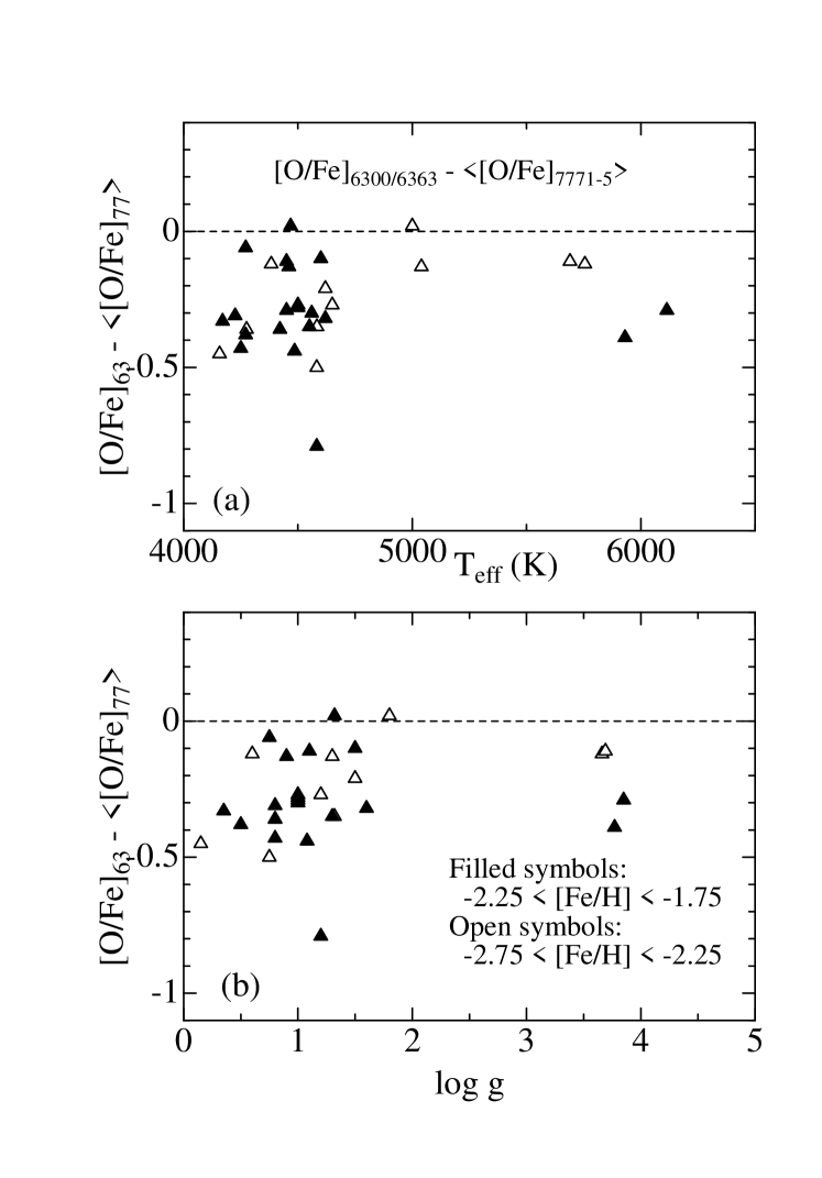
Figure 10: Dependence of [O/Fe]${}_{6300/6363}-\langle[$O/Fe$]_{7771-5}\rangle$ upon (a) $T_{\rm eff}$ and (b) $\log g$. Otherwise, the same as in Fig. 9.

This motivation reminded us of the simple unique correlation between $W_{\lambda}$(O i 7774.17) and its NLTE correction in metal-poor solar-type dwarfs (5500 K $\leq T_{\rm eff}\leq$ 6500K, $3.5\leq\log g\leq 4.5$, and $-2\leq[{\rm Fe}/{\rm H}]\leq 0$) discussed in Takeda (1994; cf. Fig. 10 therein). If such a relation really holds also in the present case irrespective of the atmospheric parameters (much wider range than that in Takeda 1994), it would greatly simplify our task. However, according to the $\Delta$ vs. $W^{\rm NLTE}$ relation for O i 7774.17 depicted in Fig. 1 (based on the data in Table 2), the situation is not such simple; i.e., $\Delta$ is not only a function of $W^{\rm NLTE}$ but also more or less dependent on $T_{\rm eff}$ and $\log g$ (and $\xi$). Nevertheless, a close examination revealed that for given $T_{\rm eff}$, $\log g$, and $\xi$, the extent of the non-LTE correction ($\Delta$) is a nearly monotonic function of the equivalent width ($W_{\lambda}$; measured in m$\rm\AA$), and that

$$\Delta=a10^{bW_{\lambda}},$$ (1)

where $a$ and $b$ are appropriately chosen coefficients as functions of ($T_{\rm eff}$, $\log g$, and $\xi$),
is a fairly good approximation for an appropriately chosen set of $(a,b)$, as far as the line is not too strong (i.e., $W_{\lambda}\la 100{\rm m\AA}$). It should be noted that this relation does not explicitly contain the metallicity, though stars with less metals generally show smaller extent of $|\Delta|$ values due to their weaker line-strengths ($W_{\lambda}$).

We therefore determined the best-fit coefficients $(a,b)$ based on the computed $\Delta$ values in Table 2 for each combination of ($T_{\rm eff}$, $\log g$, $\xi$); the resulting coefficients are summarized in Tables 3 for each of the O i triplet lines at 7771.94, 7774.17, and 7775.39 $\rm\AA$, respectively. The analytical approximations presented by Eq. (1) with the coefficients given in Table 3 are also depicted in Fig. 1 (the solid lines).

Practically, we first evaluate ($a,b$) by interpolating this table in terms of $T_{\rm eff}$, $\log g$ and $\xi$ of a star in consideration, which are then applied to Eq. (1) with the observed equivalent width to obtain the non-LTE correction.

In order to demonstrate the applicability of this formula, we show the error of Eq. (1) (defined as $\delta_{\rm error}\equiv\Delta^{\rm formula}-\Delta^{\rm actual}$) as a function of $W_{\lambda}$ for the case of O i 7774.17 in Fig. 2 (compare it with Fig. 1), where we can see that an accuracy within a few hundredths dex is accomplished as far as $W_{\lambda}\la 100$ m$\rm\AA$.

4 Discussion

4.1 NLTE correction for O I triplet: comparison with others

It is interesting to compare the non-LTE corrections for the O i 7771–5 reported in several published studies with those estimated following the procedure described in Sect. 3.3 while using the same observational equivalent widths along with the same $T_{\rm eff}$, $\log g$ and $\xi$ as given in the literature. If $W_{\lambda}$ values for two or three lines of the triplet are available, we computed the corrections for each of the lines and their average was used for the comparison.

4.1.1 Takeda et al. (1998, 2000)

Comparisons with the results of our own previous work, Takeda et al. (1998, 2000), are shown in Figs. 3a and b.

The non-LTE corrections for O i 7771.94 given in Table 2 of Takeda et al.’s (1998) population I G–K giants analysis are in good agreement with those derived from our approximate formula [Eq. (1)], in spite of the fact that extrapolating Table 3 was necessary for stars with (4250 K $\la)T_{\rm eff}<4500$ K.

We can also see that the $\Delta$ values of O i 7771–5 for very metal-poor giants computed by Takeda et al. (2000) are reasonably consistent with those estimated by the procedure proposed in this study. Note, however, that a somewhat large discrepancy is observed in the $\xi=5.1$ ${\rm km\>s^{-1}}$ case for HD 184266, where two different $\xi$ values were suggested depending on the lines (O i triplet lines and Fe I lines) used for its determination. This indicates that we should be careful at extrapolating Table 3 to considerably outside of the range they cover (e.g., 1 ${\rm km\>s^{-1}}$$\leq\xi\leq$ 3 ${\rm km\>s^{-1}}$).

Generally speaking, the results (for O i lines) of our new calculations reported in this paper (cf. Table 2) are essentially equivalent to our previous studies, in spite of the use of updated new atomic model in connection with the [O i] transition (cf. Sect. 2.1). This can be verified also by comparing Table 2 in this paper with Table 7 of Takeda (1994), both of which are practically equivalent. Taking this fact into consideration, we can again confirm from the coincidence shown in Figs. 3a and b that Eq. (1) with Table 3 is sufficiently accurate and useful for practical applications.

4.1.2 Tomkin et al. (1992)

In Tomkin et al.’s (1992) extensive analysis of C and O abundances in (from mildly to very) metal-deficient dwarfs, they performed non-LTE calculations by using a 15 levels/22 lines atomic model while adjusting the H i collision rate by the requirement that the solar O i 7771–5 lines yield the abundance of 8.92 with the solar model atmosphere of Holweger & Müller (1974). As shown in Fig. 4a, the extents of their $|\Delta|$ values ($\la 0.1$ dex) tend to be systematically smaller than ours.

4.1.3 Mishenina et al. (2000)

Comparing our $\Delta$ values with the recent non-LTE calculation of Mishenina et al. (2000), who used an atomic model comprising 75 levels/46 transitions and Steenbock & Holweger’s (1984) H i collision formula with a reduction factor of 1/3, we can see that both are in reasonably good agreement in spite of a mild difference in the treatment of H i collision rates (cf. Fig. 4b).

4.1.4 Nissen et al. (2002)

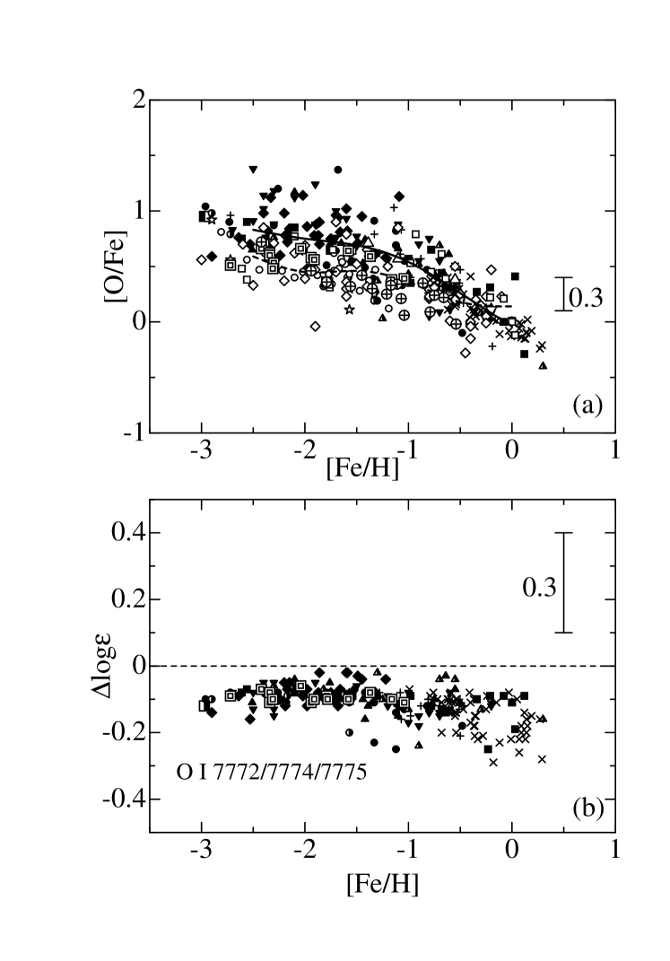
Figure 8: (a): [O/Fe] vs. [Fe/H] relation based on the reanalysis of published equivalent width data of O i 7771–5 lines (closed symbols, half-filled symbols, crosses) and [O i] 6300/6363 lines (open symbols), where the non-LTE correction was taken into account only for the O i triplet lines. The solid and dashed lines indicate the mean [O/Fe] tendencies suggested from permitted O i lines and forbidden [O i] lines, respectively. (b): Applied non-LTE corrections for the O i 7771–5 lines plotted with respect to the metallicity. Each of the symbols denote the sources of equivalent widths. O i 7771–5: filled squares—Carretta et al. (2000), St. Andrew’s crosses—Edvardsson et al. (1993), filled inverse triangles—Abia & Rebolo (1989), Greek Crosses—Boesgaard & King (1993), half-filled triangles—Sneden et al. (1979), filled triangles—Mishenina et al. (2000), filled diamonds—Tomkin et al. (1992), filled circles—Cavallo et al. (1997), half-filled circles—Takeda et al. (2000), half-filled square—King (1994), double squares—Nissen et al. (2002). [O i] 6300/6363: open squares—Carretta et al. (2000), open inverse triangles—Sneden et al. (1979), open triangles—Mishenina et al. (2000), open diamonds—Barbuy (1988) and Barbuy & Erdelyi-Mendes (1989), open circles—Sneden et al. (1991) and Kraft et al. (1992), open stars—Takeda et al. (2000), circled pluses—Nissen et al. (2002). The original data (equivalent widths and atmospheric parameters) adopted from the literature and the results of the analysis (abundances and non-LTE corrections) are given in Table 5 (available only electronically).

Nissen et al. (2002) recently carried out a careful abundance study based on their high-quality data of O i and [O i] lines (along with OH lines), and obtained almost consistent results between [O i] (LTE) and O i (non-LTE) at a “quasi-linearly increasing” trend of [O/Fe] within the framework of the 1D atmosphere analysis (though an application of the 3D correction to the [O i] abundance causes some discrepancy). Their O i non-LTE calculation is based on an atomic model comprising 22 levels/43 transitions, while completely neglecting the H i collisions. We can see from Fig. 4c that the extent of their $|\Delta|$ values tends to be larger than ours by $\la 0.15$ dex, which may be understood as being due to the different treatment of H i collisions, since neglecting this effect increases $|\Delta|$ by this amount (cf. Appendix A). Even with this moderate difference, the reanalysis of their $W_{\lambda}$(O i) and $W_{\lambda}$([O i]) data based on our $\Delta$ values nearly reproduces the results they obtained (i.e., the similar tendency for O i and [O i]), as shown in Fig. 8a.

4.1.5 Carretta et al. (2000)

Carretta et al. (2000) also obtained a nearly consistent solution of [O/Fe] between O i and [O i] in the metal-poor regime, but at a “nearly flat” trend in contrast to the results of Nissen et al. (2002) mentioned above. Namely, they reanalyzed the published $W_{\lambda}$(O i 7771–5) data of Tomkin et al. (1992) and Edvardsson et al. (1993) and showed that their (NLTE-corrected) O i abundances are consistent with those of [O i] resulting from their reanalysis of $W_{\lambda}$([O i] 6300/6363) data of Sneden et al. (1991) and Kraft et al. (1992). Their corrections are based on Gratton et al.’s (1999) NLTE calculations, where they adopted a model oxygen atom of 13 levels/28 transitions and a mild enhancement factor of $\sim 3$ (determined by the requirement of O i 7771–5/O i 6158 consistency in RR Lyr variables) applied to classical H i collision rates.

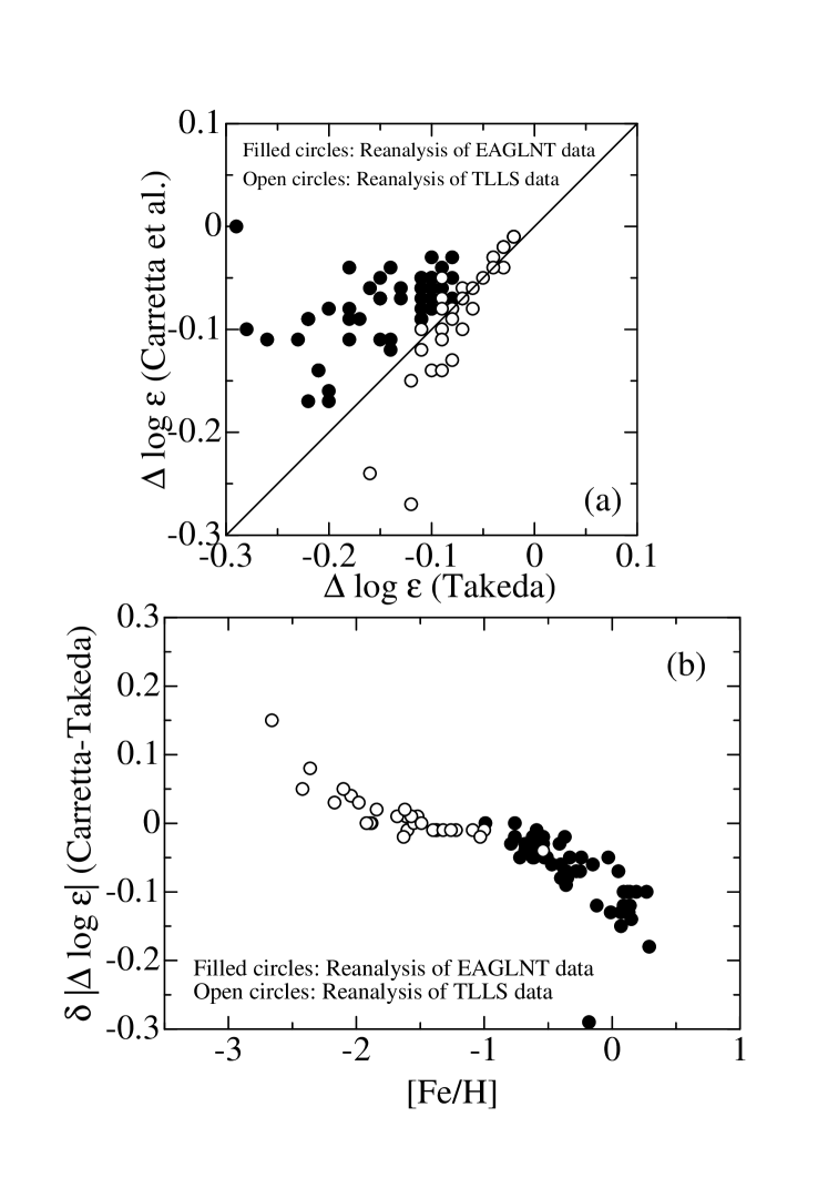
Figure 5: (a): Comparison of our non-LTE abundance corrections for O i 7771–5 triplet resulting from reanalysis of the data of Tomkin et al. (1992; open circles) and Edvardsson et al. (1993; closed circles) (as was done by Carretta et al. 2000) with the corrections determined by Carretta et al. (2000). (b): Differences between Carretta et al.’s (2000) non-LTE corrections and ours, plotted as functions of metallicity.

In Fig. 5a, their NLTE corrections are compared with our corresponding $\Delta$ values, which were evaluated from the $W_{\lambda}$(O i 7771–5) data of Tomkin et al. (1992) and Edvardsson et al. (1993) while adopting the $T_{\rm eff}$ and $\log g$ values used by Carretta et al. (2000) to make the comparison as consistent as possible. An interesting tendency is observed in this figure. That is, while the extents of their non-LTE corrections for Edvardsson et al.’s (1993) F–G disk dwarfs are systematically smaller than ours, this trend disappears and a good agreement is seen in the case of Tomkin et al.’s (1992) considerably metal-poor halo dwarf stars (their $|\Delta|$ values are even larger for two stars).

A closer inspection revealed that this is nothing but the dependence on the metallicity, as shown in Fig. 5b. Namely, their corrections (in terms of the absolute $|\Delta|$ values) are smaller than ours for mildly metal-deficient disk stars ($-1\la$ [Fe/H] $\la 0$), nearly the same for typical halo stars ($-2\la$ [Fe/H] $\la-1$), and eventually become larger than our values for very metal-poor halo stars ($-3\la$ [Fe/H] $\la-2$). Evidently, this must be the reason for their “quasi-flat” trend of [O/Fe] obtained for the O i lines, since the extent of their (negative) non-LTE correction becomes progressively larger than ours (in the relative sense) as the metallicity decreases, thus suppressing the gradient of the [O/Fe] vs. [Fe/H] relation.

4.2 Does the metallicity affect the formation of O I lines?

In Sect. 4.1.5 we found a metallicity-dependent systematic discrepancy between Carretta et al.’s (2000) non-LTE corrections and ours (i.e., theirs are systematically overcorrected toward a lowered metallicity compared to ours), which must be a very important problem because of its large impact on the [O/Fe] vs. [Fe/H] relation derived from the O i triplet lines. Hence, a detailed discussion on this matter from the viewpoint of the line-formation mechanism may be due.

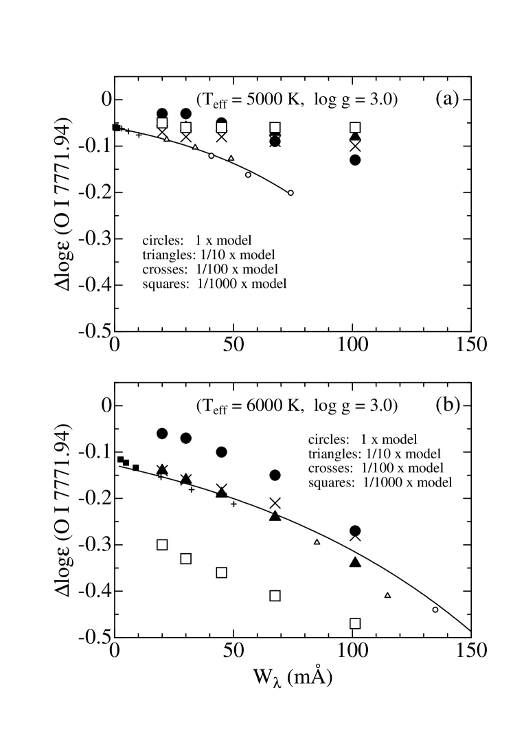
Figure 6: Non-LTE correction vs. equivalent-width relations for the O i 7771.94 line. Large symbols show the results calculated by Gratton et al. (1999), while small symbols indicate our results taken from Table 2. The model metallicity corresponding to each data point is denoted by the symbol type as explained in the figure. Our relevant (metallicity-independent) analytical relation [Eq. (1) coupled with Table 3] is depicted by the solid line, which was determined so as to fit the original data (small symbols). (a): $T_{\rm ef}$ = 5000 K, $\log g$ = 3.0; (b): $T_{\rm ef}$ = 6000 K, $\log g$ = 3.0.

Actually, such a [Fe/H]-dependent tendency of their correction is clearly observed by examining Table 10 of Gratton et al. (1999). We plotted their $\Delta$ vs. $W_{\lambda}$(7771.94) relations computed for the $\log g=3.0$ models of different metallicity in Figs. 6a and b, each corresponding to $T_{\rm eff}$ = 5000 K and 6000 K, where our computed results (Table 2) along with the corresponding analytical approximation curves [i.e., Eq. (1) with the coefficients taken from Table 3] are overplotted. It can be seen from these figures that the strong metallicity-dependence mentioned above is evidently observed in their results (especially for the case of $T_{\rm eff}$ = 6000 K). However, such a tendency (i.e., $\Delta$ is considerably dependent on the metallicity at the same $W_{\lambda}$) is not seen in our case, where $\Delta$ is nearly a monotonic function of $W_{\lambda}$ as a first approximation (see in Figs. 6a and b that the small symbols of different type continuously follow a common curve with a change in $W_{\lambda}$).

In order to demonstrate this more clearly, additional test non-LTE calculations were performed for the $T_{\rm eff}$ = 6000 K and $\log g=3.0$ models of different metallicities ($[X]=0,-1,-2,-3$) where the assigned oxygen abundances were carefully adjusted so as to yield the same (non-LTE) O i 7771.94 equivalent widths for the two metallicity pairs, $W_{\lambda}$ = 152 m$\rm\AA$ (for $[X]$ = 0 and $-1$) and $W_{\lambda}$ = 20 m$\rm\AA$ (for $[X]$ = $-2$ and $-3$) [which were chosen to keep consistency with Gratton et al.’s (1999) calculation], and computed the non-LTE correction for each case. The results are given in Table 4, where the corresponding corrections taken from Gratton et al.’s (1999) Table 10 are also quoted for a comparison. It is clear from this table that such a marked metallicity-dependence observed in Gratton et al.’s (1999) corrections (column 12) is absent in our $\Delta$ values (column 11).

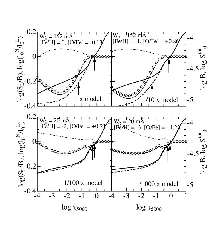
Figure 7: Run of the physical quantities involved with the line formation of the O i 7771.94 line, for the four demonstrative cases of the metallicity-dependence test given in Table 4. The thin solid line and the thin dashed line indicate the depth-dependence of the line source function (in unit of the local Planck function) and the NLTE-to-LTE line-opacity, respectively (corresponding to the scales marked in the left-hand axis). The corresponding pure two-level-atom solution of $S_{\rm L}/B$ [derived by solving the scattering problem with the line source function of Eq. (2) while using the actual depth-dependent $\epsilon^{\prime}(\tau)$, $\eta(\tau)$, and $B(\tau)$] is also shown by the open circles, which is in good agreement with the full non-LTE solution presented by Eq. (3) (thin solid line). Meanwhile, the thick solid line and the thick dashed line show the run of the Planck function itself and that of the total (i.e., line plus continuum) source function at the line center, respectively (corresponding to the scales marked in the right-hand axis). The depth points corresponding to the continuum optical-depth of unity and the line-center optical depth of unity are indicated by two upward arrows.

The reason for this characteristics in our case (i.e., near-equality of $\Delta$ at the same $W_{\lambda}$ but different metallicities) is manifestly explained by Fig. 7, where the behaviors of the source function, the NLTE-to-LTE line-opacity ratio, and the Planck function for the four test cases of Table 4 are depicted. We should note the following facts which can be read from this figure:
— (1) The line opacity for this O i line is nearly in LTE ($l_{0}^{\rm NLTE}/l_{0}^{\rm LTE}\simeq 1$) in the line-forming region. Though an appreciable departure from LTE (i.e., overpopulation) is observed at the shallower layer especially for the metal-poor atmospheres, it does not have any significant affection upon the emergent radiation. [See Sect. 4.2 in Takeda (1994) for the explanations on these characteristics of $l_{0}^{\rm NLTE}/l_{0}^{\rm LTE}$.]
— (2) As can be seen from Fig. 7, the line source function ($S_{\rm L}$) of this O i 7771.94 line resulting from our detailed non-LTE calculations (thin solid lines) is essentially the same as the two-level-atom-type line source function (open circles). Namely, the solution obtained by solving the classical scattering problem with the simple form of $S_{\rm L}^{\rm two-level}$,

$$S_{\rm L}^{\rm two-level}=(\overline{J}+\epsilon^{\prime}B)/(1+\epsilon^{\prime}),$$ (2)

while using the realistic values of $\epsilon^{\prime}(\tau)$, $B(\tau)$, and $\eta(\tau)$ computed from the model atmospheres [where $\overline{J}$ (frequency-averaged mean radiation field), $\epsilon^{\prime}$ (collisional-to-radiative ratio of the deexcitation rate), $B$ (Planck function), and $\eta(\tau)$ (the line-to-continuum opacity ratio necessary to compute the line optical depth and to combine the line-and-continuum source function into the total source function) are the quantities related to the transition between the two levels; cf. Eq. (11-6) in Mihalas (1978) or Appendix B in this paper], yields essentially the same result as $S_{\rm L}^{\rm true}$, obtained from the solutions of detailed statistical-equilibrium calculations,

$$S_{\rm L}^{\rm true}=(2h\nu^{3}/c^{2})[(n_{i}g_{j})/(n_{j}g_{i})-1]^{-1},$$ (3)

where $n_{i}$/$n_{j}$ and $g_{i}$/$g_{j}$ are the number population and the statistical weight of lower/upper level, respectively [cf. Eq. (4-14) in Mihalas (1978)]. This evidently suggests that the formation of the O I triplet is essentially determined by the quantities directly related to this transition itself without any significant relevance to the details of the adopted atomic model.
— (3) In this case, as the well-known characteristics of such a classical “two-level-atom” problem (e.g., Hummer 1968; Appendix B), the extent in the dilution of the line source function ($S_{\rm L}/B$) is controlled by the line-to-continuum opacity ratio $\eta$ ($\equiv l_{0}/\kappa$). And since both eventually determine the strength of the line, it is quite natural that the non-LTE effect (i.e., the extent of the $S_{\rm L}$ dilution) is closely coupled with the line strength ($W_{\lambda}$).

Then, there is almost no room for the metallicity directly playing any significant role in the non-LTE effect. Admittedly, there are some possibilities of metallicity-dependence even within the framework of such a two-level-type line-formation. However, any of them are unlikely in the present case. For example, appreciable [Fe/H]-dependences of $T$ (metallicity-related surface cooling) or of $l_{0}^{\rm NLTE}/l_{0}^{\rm LTE}$ [see (1) above] existing near to the surface (cf. Fig. 7) do not matter, because they occur far above the line-forming region. Also, the collisional rate between two levels (affecting the photon destruction probability $\epsilon^{\prime}$) is hardly dependent on the metallicity (or electron density) in our case because of the dominance of the H i collisions [though an extreme case of pure electron collisions (neglecting H i collisions) would lead to a metallicity-dependence of the $\epsilon^{\prime}$ values (and eventually of the non-LTE effect) owing to the role of metallicity as the electron donor; e.g., Kiselman (1991)].

A supplementary discussion based on the two-level-atom along with the simple Milne–Eddington model is given in Appendix B, where the $T_{\rm eff}$/$\log g$-dependence of the $\Delta$ vs. $W_{\lambda}$ relation given in Fig. 1 (along with its [Fe/H]-independence) is qualitatively explained more in detail.

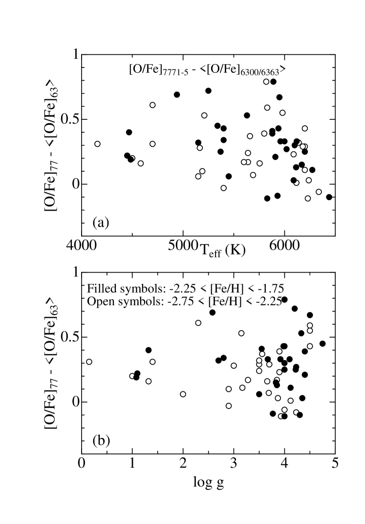
Figure 9: Dependence of [O/Fe]${}_{7771-5}-\langle[$O/Fe$]_{6300/6363}\rangle$ (the discrepancy of each star’s [O/Fe]_7771-5 relative to the mean $\langle[$O/Fe$]_{6300/6363}\rangle$) upon (a) $T_{\rm eff}$ and (b) $\log g$. Open symbols are for stars of $-2.75\leq$ [Fe/H] $<-2.25$, while filled symbols correspond to those of $-2.25\leq$ [Fe/H] $<-1.75$.

Accordingly, the results of the Padova group, that the extent of the non-LTE correction increases with a decrease in the metallicity (for a given $W_{\lambda}$), is hard to understand at least from the viewpoint of what we found from our calculations. Namely, if their results are to be seriously taken, something in their calculations must be greatly different from ours (e.g., breakdown of the two-level-atom nature and the dominant contributions from other levels and transitions). Curiously, however, an inspection of Gratton et al.’s (1999) Fig. 6 suggests that their non-LTE departure coefficients behave themselves consistently with our computational results (see, e.g., Fig. 9 of Takeda 1994); that is, for the case of $T_{\rm eff}$ = 6000 K and $\log g$ = 4.5, the departure from LTE is larger for the [Fe/H] = 0 model than for the [Fe/H] = $-2$ model. In other words, their non-LTE calculations appears quite reasonable in this respect. Then, how could their calculations lead to the tendency of enhanced $|\Delta|$ with a lowered [Fe/H] ? Anyway, it appears that the non-LTE corrections given in Gratton et al.’s (1999) Table 10 and those used by Carretta et al. (2000) are questionable, and thus their consequences had better be viewed with caution. This criticism also applies to any other results obtained by using their corrections; e.g., the “flat-like” [O/Fe] tendency derived by Primas et al. (2001).

4.3 Validity of LTE for the [O I] 6300/6363 lines

As mentioned in Sect. 1, the search for the possibility of the non-LTE effect in the [O i] lines, based on the new (more realistic) O i atom, was actually one of the main aims in this paper.

According to the present calculation, however, the departure coefficients of the lower term (2s² 2p^{4 3}P; hereinafter referred to as “term 1”) and the upper term (2p^4 1D; hereinafter “term 2”) for the [O i] 6300/6363 lines turned out to be essentially equal to unity over almost all atmospheric layers, which guarantees the validity of the assumption of LTE for these forbidden [O i] lines.

The reason for this is attributed to the fact that (1) the population of the lower ground term is thermalized relative to the continuum (i.e., accomplishment of LTE population) owing to the efficient charge-exchange reaction with H atoms, and (2) these lower and upper terms are strongly coupled with collisions which equalize the $b$ values of these two terms.

It was further found after several test calculations that this is a rather robust conclusion, which may not be affected by any uncertainty in the adopted collisional cross section. That is, although little is known and considerable ambiguities are involved in the collisional rates due to H i atoms for this 1–2 transition ($C_{1-2}^{\rm H}$; for which we used the scaled value estimated from $C_{1-2}^{\rm e}$), we obtained essentially the same results even if $C_{1-2}^{\rm H}$ was completely neglected; i.e., only the $C_{1-2}^{\rm e}$ itself is sufficiently large to bring the $b$ vales of terms 1 and 2 into the same value of unity.

We also carried out a simulation for the limiting test case of completely neglecting the collisional interaction between terms 1 and 2 ($C_{1-2}^{\rm e}=C_{1-2}^{\rm H}=0$). In this case, an appreciable overpopulation in the upper term 2 was observed (the extent of its NLTE departure growing toward the shallower layer) as a result of the downward cascade via the UV transitions connecting to term 2, which makes the NLTE line strength somewhat smaller compared to the LTE value (i.e., a positive correction in terms of $\Delta$ defined in Sect. 3.1) because of the resulting inequality of $S_{\rm L}/B>1$ in the upper layer. Even in such an extreme case, however, the extent of the computed $\Delta$ value is $\la 0.05$ dex in most range of the atmospheric parameters and definitely insignificant in the practical sense. Accordingly, we can confidently conclude that the non-LTE effect can be safely neglected for the [O i] lines, for which LTE must be a valid approximation.

4.4 [O/Fe] vs. [Fe/H] relation

4.4.1 Procedure of reanalysis

Now we are ready to study the [O/Fe] vs. [Fe/H] relation of metal-poor stars by reanalyzing the published equivalent-width data of O i 7771/7774/7775 and [O i] 6300/6363 lines while applying the non-LTE corrections based on our calculations.

We adopted the same $T_{\rm eff}$, $\log g$, [Fe/H], and $\xi$ values as those used in the literature, from which the data of equivalent widths were taken. Regarding the model atmospheres, we used Kurucz’s (1993) grid of ATLAS9 models ($\xi$ = 2 ${\rm km\>s^{-1}}$) which were interpolated with respect to $T_{\rm eff}$, $\log g$, and [Fe/H] of a star. As in Sect. 3.2, Kurucz’s WIDTH9 program was invoked for determining the LTE abundance ($\log\epsilon_{\rm O}^{\rm LTE}$) while using the line data given in Table 1. Then, the [O/Fe] ratio is obtained as

$$[{\rm O}/{\rm Fe}]\equiv(\log\epsilon_{\rm O}^{\rm LTE}+\Delta-8.93)-[{\rm Fe}/{\rm H}],$$ (4)

where $\Delta$ is the non-LTE abundance correction, which was evaluated from $W_{\lambda}$, $T_{\rm eff}$, $\log g$, and $\xi$ based on the procedure described in Sect. 3.3 [i.e., application of Eq. (1) with Table 3] for the case of O i 7771/7774/7775 lines, and $\Delta=0$ was adopted for the [O i]  6300/6363 lines (cf. Sect. 4.3). Note that the solar oxygen abundance was assumed to be 8.93 (in the usual scale of $\log\epsilon_{\rm H}=12$) according to Anders & Grevesse (1989). We treat [O/Fe] derived from O i 7771–5 lines and [O i] 6300/6363 lines separately, which we hereinafter referred to as [O/Fe]₇₇ and [O/Fe]₆₃, respectively. In case that equivalent-width data are available for two or three O i triplet lines, or for both [O i] lines, we calculated [O/Fe] for each line and adopted their simple mean to obtain [O/Fe]₇₇ or [O/Fe]₆₃.

4.4.2 Results of [O/Fe]

We tried to use as many $W_{\lambda}$ data as possible taken from various sources, though our literature survey is not complete. Consequently, $\sim 300$ stars ($\sim 200$ for [O/Fe]₇₇ and $\sim 100$ for [O/Fe]₆₃) covering a metallicity range of $-3\la$ [Fe/H] $\la 0$ could be analyzed, which may be sufficient for statistically meaningful discussion. The adopted data of the atmospheric parameters ($T_{\rm eff}$, $\log g$, $\xi$) the equivalent widths for each star are given in Table 5 (available only in electronic form), where the results of the LTE abundances and the non-LTE corrections/abundances are also presented. The resulting [O/Fe] ratios (i.e., [O/Fe]₇₇ or [O/Fe]₆₃) plotted with respect to [Fe/H] for each star are shown in Fig. 8a, and the corresponding non-LTE corrections applied to the O i 7771–5 lines are also plotted in Fig. 8b. The mean $\langle[$O/Fe$]_{77}\rangle$ and $\langle[$O/Fe$]_{63}\rangle$, averaged in each [Fe/H] bin of 0.5 dex, are given in Table 6. The spline-fit curves for the runs of $\langle[$O/Fe$]_{77}\rangle$ and $\langle[$O/Fe$]_{63}\rangle$ with [Fe/H] are also depicted in Fig. 8a. Our conclusions read from Fig. 8 and Table 6 are as follows.

(1) For mildly metal-deficient disk stars ($-1\la$ [Fe/H] $\la 0$), our [O/Fe]₇₇ and [O/Fe]₆₃ show a quite similar behavior; i.e., a gradual increase from [O/Fe]$\sim 0$ ([Fe/H] $\sim 0$) to [O/Fe]$\sim+0.5$ ([Fe/H] $\sim-1$). This means that our non-LTE corrections are successful to achieve an agreement between the oxygen abundances derived from [O i] 6300/6363 and O i 7771–5 for those population I stars, which is consistent with the conclusion of Takeda et al. (1998).

(2) However, a discrepancy begins to appear when we go toward a lower metallicity further down from [Fe/H] $\sim-1$. That is, [O/Fe]₇₇ still increases with a slight change (i.e., gentler) of the slope from [O/Fe]$\sim+0.5$ ([Fe/H] $\sim-1$) to [O/Fe]$\sim+1$ ([Fe/H] $\sim-3$), while [O/Fe]₆₃ maintains nearly the same value at [O/Fe]$\sim+0.5$ on the average over the metallicity range of $-2.5\la$ [Fe/H] $\la-1$ showing a quasi-flat plateau. This kind of [O/Fe]₇₇ vs. [O/Fe]₆₃ discordance for those conspicuously metal-poor halo stars is just what has been occasionally reported so far (cf. Sect. 1). Our analysis thus suggests that this discrepancy in halo stars (amounting to $\sim$ 0.2–0.3 dex at $-2.5\la$ [Fe/H] $\la-1.5$) does exist, without being successfully removed by our non-LTE corrections, unlike the conclusion of Carretta et al. (2000). We will discuss this problem more in detail in the next section.

4.5 O I vs. [O I] discrepancy

4.5.1 Discordance in halo stars

We have thus confirmed the existence of discrepancy between [O/Fe]₇₇ and [O/Fe]₆₃ in the quite metal-poor regime ($-3\la$ [Fe/H] $\la-1$), while a good agreement was obtained in disk stars ($-1\la$ [Fe/H] $\la 0$).

This can not be successfully removed by the non-LTE effect though they surely act in the direction of mitigating the discordance. According to our opinion (cf. Sect. 4.2), the O i vs. [O i] consistency obtained by Carretta et al. (2000) may be nothing but a fortuitous coincidence caused by their questionable non-LTE corrections for the O i 7771–5 triplet (i.e., systematically overcorrected toward a lower metallicity).

It is also unlikely that systematic errors in the $T_{\rm eff}$ scale (affecting mainly on O i) is responsible for the cause of this discrepancy as has been occasionally suspected (e.g., King 1993), since our analysis in Sect. 4.4 is based on the mixed data of equivalent widths and atmospheric parameters taken from a variety of data sources.

Hence, we would consider that this discordance in halo stars is more or less inevitable as far as the conventional abundance determination method is concerned (i.e., “standard” non-LTE calculations as well as model atmospheres); that is, a challengingly novel modelling would be required to bring them into agreement.

4.5.2 Search for a trend in terms of $T_{\rm eff}$ and $\log g$

Then, the next question of interest is naturally “which solution is correct ?”, or in other words “which yields the wrong abundances, O i 7771–5 or [O i] 6300/6363 ?”. While this is a difficult question, it may be worthwhile as a first step to study the nature of the discordance; i.e., its dependence on $T_{\rm eff}$ and $\log g$.

Let us invoke the following guiding principle: If we assume that the origin of the error is concerned with some stellar physical property which is not appropriately modelled, it is reasonable to expect that abundance discrepancies shown by the erroneous side (whichever O i or [O i]) may show some kind of systematic tendency in terms of these stellar parameters, since any stellar physical environment must undergo a distinct change if these parameters vary substantially. And, in an ideal case, the discordance might asymptotically disappear if we go to either limit of the parameter variation.

Motivated by this thought, we paid attention to [O/Fe]${}_{77}-\langle[$O/Fe$]_{63}\rangle$ (the discrepancy of each star’s [O/Fe]₇₇ relative to the mean $\langle[$O/Fe$]_{63}\rangle$) and [O/Fe]${}_{63}-\langle[$O/Fe$]_{77}\rangle$ (the inverse of the above) within two metallicity bins of $-2.75\leq$ [Fe/H] $<-2.25$ and $-2.25\leq$ [Fe/H] $<-1.75$, where a clear discordance of $\langle[$O/Fe]${}_{77}\rangle-\langle[$O/Fe$]_{63}\rangle\sim 0.3$ dex is observed (cf. Table 6). The dependence of former quantity for each stars is plotted in Fig. 9 with respect to $T_{\rm eff}$ (a) and $\log g$ (b), while that of the latter is similarly shown in Fig. 10.

In Fig. 9, what we observe is mostly a large scatter around the mean of $\sim+0.3$, which is presumably caused by the strong $T_{\rm eff}$-sensitivity of these high-excitation O i 7771–5 lines. However, we can recognize in Fig 9a a marginal trend that [O/Fe]${}_{77}-\langle[$O/Fe$]_{63}\rangle$ tends to decrease toward higher $T_{\rm eff}$ (especially at $T_{\rm eff}\ga 6000$ K). Also, if we pay attention to the data for $-2.75\leq$ [Fe/H] $<-2.25$ in Fig. 9b (open circles), a slight $\log g$-dependence appears to exist in the sense that higher-gravity stars tend to show less extent of the discordance. Similarly, Fig. 10 also suggests a weak trend for this group of very metal-poor stars (open circles); i.e., $|$[O/Fe]${}_{63}-\langle[$O/Fe$]_{77}\rangle|$ appears to decrease with an increase in $T_{\rm eff}$ as well as in $\log g$ toward the high-$T_{\rm eff}$/high-$\log g$ limit. Consequently, a weak systematic trend may exist, especially for the very metal-deficient case of $-2.75\leq$ [Fe/H] $<-2.25$, in the sense that the discrepancy tends to be lessened for an increase in $T_{\rm eff}$ as well as in $\log g$.

However, these suspected $T_{\rm eff}$- and $\log g$-dependences should not be regarded as being independent. We should recall that the very metal-poor stars ([Fe/H] $\la-2$) analyzed so far are mainly giants or subgiants. Namely, since $T_{\rm eff}$ and $\log g$ show a close positive correlation in metal-poor giants reflecting the position on the HR diagram (see, e.g., Fig. 3 of Pilachowski et al. 1996), the rather similar behavior of the O i $-$ [O i] discrepancy in terms of the changes in both $T_{\rm eff}$ and $\log g$ may be naturally understood.

Consequently, what we can learn from Figs. 9 and 10 is, modestly speaking, that analyzing higher $T_{\rm eff}/\log g$ subgiants (and maybe also dwarfs) has a less probability of suffering a large O i $-$ [O i] discrepancy as compared to the study of lower $T_{\rm eff}/\log g$ giants. The recent results of Nissen et al. (2001) (cf. footnote 10) may be regarded as supporting this speculation, since their data are based on stars with $\log g>3$.

Unfortunately, however, Figs. 9 and 10 do not allow us any definitive arguments regarding the cause of the discrepancy or which of the O i or [O i] is problematic. It is apparent from these figures that the [O i] data of very metal-poor subgiants and dwarfs with higher $T_{\rm eff}/\log g$ (and inversely the O i data for very metal-poor giants with lower $T_{\rm eff}/\log g$) are quite insufficient, reflecting the preference of [O i] lines for giants so far (because their strengths increase with a lowering of the gravity). Hence, in order for a reliable statistical discussion, much more observations of [O i] lines for very metal-poor dwarfs or subgiants of higher gravity (along with O i lines for very metal-poor giants of lower gravity) are desirably awaited, which would surely improve this situation toward clarifying the origin of the discrepancy.

5 Conclusion

For the purpose of investigating the line formation of O i 7771–5 lines of IR triplet and [O i] 6300/6363 lines especially concerning the consistency of the oxygen abundances derived from these two in metal-poor disk/halo stars, we carried out non-LTE calculations with a new atomic model of oxygen on an extensive grid of model atmospheres (4500 K $\leq T_{\rm eff}\leq$ 6500 K, $1\leq\log g\leq 5$, and $-3\leq[{\rm Fe}/{\rm H}]\leq 0$).

In order to make the resulting non-LTE abundance corrections of O i 7771–5 lines more useful for practical applications, we derived an analytical formula with appropriate coefficients computed and tabulated in a grid of atmospheric parameters, by which the non-LTE correction is easily evaluated for any given set of $W_{\lambda}$, $T_{\rm eff}$, $\log g$ and $\xi$.

We discussed our non-LTE corrections for the O i triplet lines while comparing them with those derived from other studies published so far. We could not reproduce the trend of the non-LTE correction derived by Carretta et al. (2000), the systematic [Fe/H]-dependence of which is essentially the reason for their success of accomplishing the O i vs. [O i] consistency.

In contrast, we have shown that the non-LTE effect of O i 7771–5 lines is well described by the classical two-level-atom model and the metallicity can not be an essential factor. As a matter of fact, the formation of this O i triplet was found to be quite simple in the sense that only the transition-related quantities are important and details of the atomic model are not very significant, supporting the arguments of Kiselman (2001) and Nissen et al. (2002) who also arrived at the same conclusion.

Regarding the forbidden [O i] lines, we arrived at a robust conclusion that the non-LTE effect for the [O i] 6300/6363 lines can be safely negligible and thus LTE is a valid approximation.

We reanalyzed the various published equivalent-width data of O i 7771–5 and [O i] 6300/6363 lines (while the non-LTE effect is taken into account for the former based on our calculations), in order to study the behavior of [O/Fe] vs. [Fe/H] relation over a wide range of metallicity ($-3\la[{\rm Fe}/{\rm H}]\la 0$). While [O/Fe]₇₇ and [O/Fe]₆₃ were found to agree with each other for disk stars ($-1\la[{\rm Fe}/{\rm H}]\la 0$), the existence of a systematic discrepancy was confirmed for halo stars ($-3\la[{\rm Fe}/{\rm H}]\la-1$) amounting to [O/Fe]${}_{77}-$ [O/Fe]${}_{63}\sim 0.3$ dex at $-3\la[{\rm Fe}/{\rm H}]\la-2$.

An inspection of the dependence of discrepancy upon $T_{\rm eff}$ and $\log g$ suggested that the extent of the discrepancy tends to be comparatively lessened for higher $T_{\rm eff}/\log g$ stars, indicating the preference of dwarf (or subgiant) stars for studying the oxygen abundance of metal-deficient stars.

Appendix A On the effect and treatment of H i collision

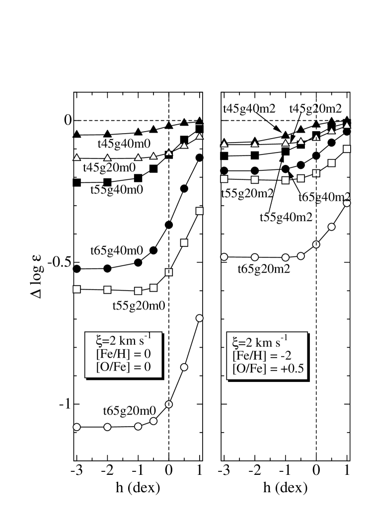
Figure 11: Dependence of the non-LTE correction for the O i 7774.18 line upon the logarithmic correction ($h$) applied to the classical treatment of H i collision rates. Left panel: ([O/Fe] = 0.0, $\xi$ = 2 km s^-1) calculations for representative [Fe/H] = 0 models; right panel: ([O/Fe] = +0.5, $\xi$ = 2 km s^-1) calculations for representative [Fe/H] = $-2$ models. Code “t$aa$g$bb$m$c$” denotes the model with $T_{\rm eff}({\rm K})=aa\times 100$, $\log g$ (cm s^-2) = $bb/10$, and [Fe/H] (metallicity) = $-c$.

The inelastic collision rate due to neutral hydrogen atoms is regarded to be one of the important ambiguous factors in non-LTE calculations on late-type stellar atmospheres. A rough classical formula derived by Steenbock and Holweger (1984) is available for this (see Takeda 1991 for more detailed description on the standard classical recipe adopted). However, because of its nature of only an order-of-magnitude accuracy, a correction factor is often introduced, by which this classical rate is to be multiplied. We express this factor as $10^{h}$ by using the logarithmic correction ($h$). Negative $h$ leads to the suppression of the H i collisional rates compared to the classical case, which increases the extent of the NLTE abundance correction ($|\Delta|$); and vice versa. This situation is depicted in Fig. 11, where the $h$-dependence of $\Delta$ for the O i 7774.18 line is shown, which was calculated for selected representative models.

As mentioned in Sect. 2.1, we used $h=0$ (as was done by Takeda 1992, 1994) throughout this paper, which means the simple adoption of the classical treatment without any correction. This choice stems from the detailed investigation of Takeda (1995), where $h=0.0(\pm 0.5)$ was concluded from the analysis of the solar flux spectrum based on (1) the comparison of the solar oxygen abundance derived from O i 7771–5 lines with the average of other 15 weaker lines and (2) the profile-fitting of these near-IR triplet lines.

It may be worthwhile, from another point of view, to check the consistency of this treatment on nearby solar-type stars, which have been recently analyzed by Takeda et al. (2001) to study the abundance characteristics of planet-harboring stars.

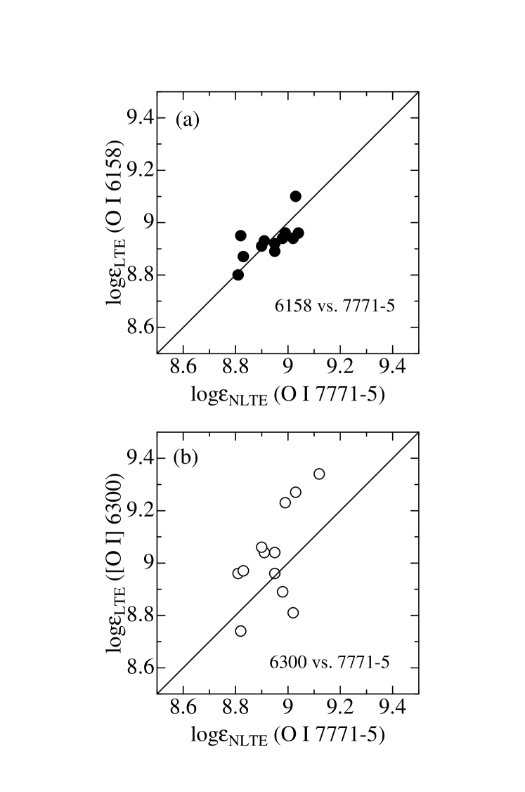
Figure 12: Comparison of the oxygen abundances derived from the O i 7771–5 lines (with the NLTE corrections presented in this study) with those determined from other oxygen lines for nearby solar-type stars analyzed by Takeda et al. (2001): (a) O i 6158.2 line (comprising three components), (b) [O i] 6300 forbidden line.

Fig. 12 shows the comparison of the non-LTE abundance of O i 7771–5 triplet (with the NLTE correction obtained by using the formula described in this study) with the LTE abundance of O i 6158.2 (a) and [O i] 6300.3 (b), which were derived from either equivalent-widths or spectrum-synthesis technique (with the same line data as given in Table 1) as described in Takeda et al. (2001). Note that LTE can be safely applied to these latter two lines (cf. Table 7 and Sect. 4.3).

We can see from Fig. 12a that $\log\epsilon_{6158}^{\rm O}$ and $\log\epsilon_{7771-5}^{\rm O}$ are in satisfactory agreement with each other, which confirms that our choice of $h=0$ is surely reasonable at least within the framework of our non-LTE calculations.

Meanwhile, for the case of 6300 vs. 7771–5 comparison shown in Fig. 12b, the scatter is comparatively large, which makes this figure less useful for the purpose of checking the adequacy of $h$. Presumably, this appreciable spread may be due to the large difference in the $T_{\rm eff}$-sensitivity of these two lines (in contrast to the case of 7771–5 and 6158 which have almost the same $T_{\rm eff}$-dependence). A close inspection of Fig. 12b suggests that the 6300 abundance tends to be somewhat larger especially for the case of higher oxygen abundance ($\log\epsilon\ga 9.0$), for which two reasons may be suspected; i.e., the possible inaccuracy in the adopted $gf$ value and/or the effect of blending. That is, according to the recent study of the solar [O i] 6300 line profile by Allende Prieto et al. (2001), the Ni i line at 6300.34 $\rm\AA$ makes an appreciable contribution to this feature. Our neglect of this effect may have cause an overestimation. In addition, their paper suggests that the most recently calculated $gf$ value is $\log gf$([O i] 6300) = $-9.72$, which is by +0.1 dex larger than that adopted in this study (cf. Table 1). Hence, our solution of $\log\epsilon_{6300}^{\rm O}$ may have been somewhat overestimated also from this point of view.

We finally remark that, even if our $\log\epsilon_{6300}^{\rm O}$ values have been overestimated either due to the use of underestimated $\log gf$ or due to the blending effect of the Ni line, our conclusion of 6300 vs. 7771–5 abundance discrepancy (cf. Sect. 4.4.2) can not be changed at all (i.e., because the discordance would become even larger).

Appendix B Interpretation of the triplet-line formation with the two-level-atom model

It was shown in Sect. 4.2 that the formation of O i 7771–5 lines can be well described by the “two-level” atomic model. Based on this simple line source function [cf. Eq. (2)] with the classical Milne–Eddington model (i.e., depth-independent line-parameters with the continuum source function linearly increasing with $\tau$), we try to explain the results of our non-LTE calculations, that the NLTE correction for the O i 7773 triplet (for given $T_{\rm eff}$, $\log g$, and $\xi$) is nearly a monotonic function of $W_{\lambda}$ (irrespective of any reasonable change in the metallicity). Though this is a very simple schematic model, it gives us a deep insight on the formation of this O i line.

B.1 What we can learn from the basic characteristics

It was Hummer (1968) who first showed that the extent of the dilution in the two-level-atom line source function defined by Eq. (2) is determined by (a) the photon-destruction probability defined as the ratio of the radiative to collisional (downward) transition probability ($\epsilon^{\prime}\simeq C_{21}/A_{21}$; cf. equation [11-7] in Mihalas 1978) and (b) the relative importance of the thermalizing continuum determined by the line-to-continuum opacity ratio $\eta\equiv\kappa_{\rm L}/\kappa_{\rm C}$ (cf. Hummer 1968). Namely:
(i) For the same $\epsilon^{\prime}$ (i.e., atmospheres with the same temperature and density), the extent of $\eta$ essentially controls the dilution of $S_{\rm L}$ is (i.e. the larger $\eta$, the more enhanced NLTE effect).
(ii) On the other hand, the extent of the dilution in $S_{\rm L}$ naturally determines the importance of the NLTE effect (i.e., the extent of the NLTE correction) as well as the strength of the observed line (i.e., equivalent width) in this case of scattering line formation.
We now understand from “fact (ii)” that a close relationship exists between the strength of the O i 7771–5 triplet lines and the corresponding non-LTE corrections. Meanwhile, “fact (i)” simply tells that the essential key parameter is $\eta$ only (for the same $\epsilon^{\prime}$), which further suggests that the difference in the metallicity does not play any essential role in the present problem. Namely, as far as the line-to-continuum opacity ratio is the same (along with the same $T_{\rm eff}$ and $\log g$), the same extent of $S_{\rm L}$, the same equivalent width, and the same non-LTE correction are expected irrespective of the metallicity, thus yielding the same $\Delta$ vs. $W_{\lambda}$ correlation.

B.2 Numerical simulation toward a qualitative explanation of Fig. 1

It may be instructive to compare the results from a simple simulation based on such a ”two-level” model with the actually obtained $\Delta$ vs. $W_{\lambda}$ relation shown in Fig. 1. Though the value of $\epsilon^{\prime}$ is strongly depth-dependent in real atmospheres, we found $\epsilon^{\prime}\sim 1$ (dwarfs) and $\epsilon^{\prime}\sim 0.1$ (supergiants) in the line-forming region from actual model calculations. We adopted the Milne–Eddington model assuming the depth-independent line-to-continuum opacity ratio $\eta$ and the linear form of the Planck function, $B(\tau)\equiv B_{0}+B_{1}\tau=B_{0}(1+B_{1}/B_{0}\tau)$ ($\tau$: continuum optical depth). We fixed $B_{0}=1$ and changed the gradient $B_{1}(=B_{1}/B_{0})$. Again the determination of this gradient at 7773 $\rm\AA$ is rather difficult since it is not linear in terms of $\tau$ in actual cases, but we tentatively chose by inspection of the model atmospheres $B_{1}=2$ (low $T_{\rm eff}$ case) and $B_{1}=1$ (high $T_{\rm eff}$ case). Hence, the radiative transfer problems (two-level-atom, complete frequency redistribution, and the pure Gaussian line profile) investigated by Hummer (1968) were numerically solved by using the Rybicki’s (1971) scheme for various values of $\eta$ ranging from $10^{-2}$ to $10^{3}$ for each of the three combinations of ($B_{1}$, $\epsilon^{\prime}$); (2, 1), (2, 0.1), and (1, 1). And then the emergent flux spectra were computed from the resulting solution of the source function (NLTE case), along with the LTE case of $S_{\rm L}=B$ (i.e., the limit of $\epsilon^{\prime}\rightarrow\infty$), to obtain the equivalent width ($W$).

In Fig. 13 are shown the LTE and NLTE curves of growth [panel (a)], and the corresponding NLTE correction $\Delta\log\eta$ ($\equiv\log\eta_{\rm NLTE}-\log\eta_{\rm LTE}$; i.e., difference of the abscissa for a given $W$) as a function of $W_{\rm NLTE}$ [panel (b)]. We can see from Fig. 13b that the computed $\Delta\log\eta$ vs. $W_{\rm NLTE}$ curves well resemble (at least qualitatively) the $\Delta$ vs. $W_{\lambda}$ relations observed in Fig. 1, in the sense that they can be approximated with the functional form of Eq. (1).

It is worthwhile paying attention to the effects of changing $\epsilon^{\prime}$ or $B_{1}$ observed in Fig. 13b. As expected, the extent of the NLTE correction increases with a decrease in $\epsilon^{\prime}$. Meanwhile, that $|\Delta\log\eta|$ is larger for a smaller gradient ($B_{1}$) of the Planck function may be attributed to the decreased sensitivity of $W_{\rm LTE}$ (to a change in $\eta$) owing to the lessened gradient (i.e., $W_{\rm LTE}$ is relatively more affected by the Planck function $B$, in contrast to the NLTE case which is mainly controlled by the radiation field). It should be noted that these two qualitative behaviors concluded from our simple model reasonably explain the tendencies observed in Fig. 1. That is, the larger $|\Delta|$ for a lowered gravity (at a given $W_{\lambda}$) is reasonably explained by the $\epsilon^{\prime}$-dependence described above. Meanwhile, regarding the tendency of larger $|\Delta|$ for a higher $T_{\rm eff}$ (at a given $W_{\lambda}$), the above-mentioned effect of decreased $B_{1}$ may be responsible for it.

Table 1: Data of neutral oxygen lines adopted for abundance calculations.

RMT	$\lambda$ ($\rm\AA$)	$\chi$ (eV)	$\log gf$	Gammar	Gammas	Gammaw
1	7771.944	9.146	0.324	7.52	$-5.55$	$-7.65^{*}$
1	7774.166	9.146	0.174	7.52	$-5.55$	$-7.65^{*}$
1	7775.388	9.146	$-0.046$	7.52	$-5.55$	$-7.65^{*}$
$\cdots$	6300.304	0.000	$-9.819$	$-2.17$	$-7.83^{*}$	$-8.13^{*}$
$\cdots$	6363.776	0.020	$-10.303$	$-2.17$	$-7.83^{*}$	$-8.13^{*}$
10	6158.149	10.741	$-1.891$	7.62	$-3.96$	$-7.23^{*}$
10	6158.172	10.741	$-1.031$	7.62	$-3.96$	$-7.23^{*}$
10	6158.187	10.741	$-0.441$	7.62	$-3.96$	$-7.23^{*}$

Note — All data are were taken from Kurucz & Bell’s (1995) compilation as far as available.
Followed by first four self-explanatory columns, damping parameters are given in the last three columns:
Gammar is the radiation damping constant, $\log\gamma_{\rm rad}$.
Gammae is the Stark damping width per electron density at $10^{4}$ K, $\log(\gamma_{\rm e}/N_{\rm e})$.
Gammaw is the van der Waals damping width per hydrogen density at $10^{4}$ K, $\log(\gamma_{\rm w}/N_{\rm H})$.
^∗ Computed as default values in the Kurucz’s WIDTH program (cf. Leusin, Topil’skaya 1987).

Table 3: Coefficients ($a$, $b$) for O I 7771.94, 7774.17, and 7775.39.

Line	$T_{\rm eff}$	$\log g$	$a$ ($\xi=1$)	$b$ ($\xi=1$)	$W$ range	$a$ ($\xi=2$)	$b$ ($\xi=2$)	$W$ range	$a$ ($\xi=3$)	$b$ ($\xi=3$)	$W$ range
7771.94	4500	1.0	$-$0.075002	0.009542	( 1, 65)	$-$0.075356	0.008023	( 1, 74)	$-$0.074381	0.006728	( 1, 85)
7771.94	4500	2.0	$-$0.063934	0.009469	( 0, 41)	$-$0.063630	0.008285	( 0, 46)	$-$0.063137	0.006891	( 0, 52)
7771.94	4500	3.0	$-$0.035192	0.011033	( 0, 27)	$-$0.034745	0.011525	( 0, 28)	$-$0.034471	0.009788	( 0, 30)
7771.94	4500	4.0	$-$0.017092	0.007009	( 0, 15)	$-$0.016955	0.007648	( 0, 16)	$-$0.017007	0.006311	( 0, 17)
7771.94	4500	5.0	$-$0.007669	$-$0.012856	( 0,  8)	$-$0.007191	$-$0.014193	( 0,  8)	$-$0.006915	$-$0.013005	( 0,  8)
7771.94	5000	1.0	$-$0.107305	0.006369	( 2,135)	$-$0.107536	0.005386	( 2,155)	$-$0.106370	0.004483	( 2,182)
7771.94	5000	2.0	$-$0.093306	0.007027	( 1, 96)	$-$0.093021	0.005981	( 1,110)	$-$0.092000	0.005021	( 1,126)
7771.94	5000	3.0	$-$0.060149	0.008351	( 0, 66)	$-$0.060438	0.007135	( 0, 74)	$-$0.059794	0.006105	( 0, 83)
7771.94	5000	4.0	$-$0.026452	0.010508	( 0, 44)	$-$0.026505	0.009854	( 0, 48)	$-$0.026579	0.008254	( 0, 52)
7771.94	5000	5.0	$-$0.010772	0.007419	( 0, 31)	$-$0.010895	0.006636	( 0, 32)	$-$0.010664	0.006359	( 0, 34)
7771.94	5500	1.0	$-$0.173154	0.004333	( 5,200)	$-$0.171278	0.003712	( 5,234)	$-$0.168826	0.003108	( 5,282)
7771.94	5500	2.0	$-$0.130188	0.005075	( 2,162)	$-$0.129085	0.004355	( 2,186)	$-$0.127260	0.003656	( 2,219)
7771.94	5500	3.0	$-$0.088392	0.005886	( 1,123)	$-$0.088652	0.005063	( 1,138)	$-$0.087546	0.004300	( 1,158)
7771.94	5500	4.0	$-$0.045400	0.006999	( 0, 89)	$-$0.045010	0.006242	( 0, 98)	$-$0.044836	0.005401	( 0,110)
7771.94	5500	5.0	$-$0.017273	0.007421	( 0, 66)	$-$0.017193	0.006644	( 0, 71)	$-$0.017248	0.005989	( 0, 76)
7771.94	6000	1.0	$-$0.266939	0.003000	(13,251)	$-$0.260351	0.002631	(12,295)	$-$0.247962	0.002325	(13,347)
7771.94	6000	2.0	$-$0.199517	0.003669	( 6,214)	$-$0.196006	0.003214	( 6,245)	$-$0.191289	0.002757	( 6,288)
7771.94	6000	3.0	$-$0.129293	0.004429	( 3,174)	$-$0.128434	0.003859	( 2,200)	$-$0.126288	0.003282	( 3,234)
7771.94	6000	4.0	$-$0.069964	0.005137	( 1,138)	$-$0.070334	0.004515	( 1,155)	$-$0.068899	0.003922	( 1,178)
7771.94	6000	5.0	$-$0.029232	0.005318	( 0,112)	$-$0.028856	0.004924	( 0,120)	$-$0.029252	0.004288	( 0,132)
7771.94	6500	1.0	$-$0.425820	0.002043	(25,282)	$-$0.406389	0.001874	(25,331)	$-$0.382757	0.001703	(25,389)
7771.94	6500	2.0	$-$0.316286	0.002456	(13,251)	$-$0.305817	0.002219	(13,295)	$-$0.291792	0.001979	(13,347)
7771.94	6500	3.0	$-$0.198270	0.003252	( 6,219)	$-$0.195040	0.002890	( 6,251)	$-$0.187683	0.002557	( 6,288)
7771.94	6500	4.0	$-$0.106599	0.003996	( 2,182)	$-$0.104490	0.003609	( 2,204)	$-$0.102594	0.003146	( 2,234)
7771.94	6500	5.0	$-$0.044660	0.004404	( 1,155)	$-$0.045000	0.003978	( 1,170)	$-$0.044197	0.003590	( 1,186)
7774.17	4500	1.0	$-$0.073793	0.010148	( 0, 58)	$-$0.073780	0.008488	( 0, 66)	$-$0.072979	0.007092	( 0, 76)
7774.17	4500	2.0	$-$0.063712	0.006132	( 0, 35)	$-$0.062821	0.008346	( 0, 40)	$-$0.062356	0.006906	( 0, 45)
7774.17	4500	3.0	$-$0.035064	0.010989	( 0, 23)	$-$0.034614	0.011527	( 0, 23)	$-$0.034347	0.009430	( 0, 26)
7774.17	4500	4.0	$-$0.016938	0.007280	( 0, 13)	$-$0.017033	0.005749	( 0, 13)	$-$0.016773	0.004774	( 0, 14)
7774.17	4500	5.0	$-$0.007297	$-$0.010223	( 0,  6)	$-$0.006829	$-$0.012540	( 0,  6)	$-$0.007200	$-$0.023415	( 0,  7)
7774.17	5000	1.0	$-$0.105560	0.006706	( 1,123)	$-$0.105520	0.005653	( 1,141)	$-$0.104210	0.004709	( 1,166)
7774.17	5000	2.0	$-$0.091507	0.007408	( 1, 87)	$-$0.091394	0.006292	( 1, 98)	$-$0.090448	0.005256	( 1,112)
7774.17	5000	3.0	$-$0.059339	0.008759	( 0, 58)	$-$0.059182	0.007595	( 0, 65)	$-$0.058655	0.006327	( 0, 72)
7774.17	5000	4.0	$-$0.026360	0.010633	( 0, 37)	$-$0.026406	0.009823	( 0, 41)	$-$0.026522	0.008324	( 0, 45)
7774.17	5000	5.0	$-$0.010885	0.006427	( 0, 26)	$-$0.010977	0.005904	( 0, 26)	$-$0.010598	0.005227	( 0, 28)
7774.17	5500	1.0	$-$0.168793	0.004559	( 4,191)	$-$0.166332	0.003922	( 4,219)	$-$0.163428	0.003289	( 4,257)
7774.17	5500	2.0	$-$0.126021	0.005383	( 2,148)	$-$0.125805	0.004568	( 2,170)	$-$0.124542	0.003804	( 2,200)
7774.17	5500	3.0	$-$0.087354	0.006180	( 1,110)	$-$0.086594	0.005325	( 1,123)	$-$0.085991	0.004476	( 1,141)
7774.17	5500	4.0	$-$0.044505	0.007448	( 0, 78)	$-$0.044722	0.006527	( 0, 85)	$-$0.044613	0.005536	( 0, 96)
7774.17	5500	5.0	$-$0.016934	0.007810	( 0, 56)	$-$0.017195	0.006915	( 0, 60)	$-$0.017136	0.006154	( 0, 65)
7774.17	6000	1.0	$-$0.254642	0.003237	( 9,240)	$-$0.243609	0.002897	( 9,275)	$-$0.236696	0.002478	( 9,331)
7774.17	6000	2.0	$-$0.192306	0.003910	( 4,200)	$-$0.189738	0.003393	( 4,229)	$-$0.185979	0.002875	( 4,269)
7774.17	6000	3.0	$-$0.125586	0.004661	( 2,162)	$-$0.124640	0.004046	( 2,182)	$-$0.122884	0.003402	( 2,214)
7774.17	6000	4.0	$-$0.068886	0.005361	( 1,126)	$-$0.068406	0.004741	( 1,138)	$-$0.067629	0.004055	( 1,155)
7774.17	6000	5.0	$-$0.028857	0.005626	( 0, 96)	$-$0.028811	0.005050	( 0,105)	$-$0.028577	0.004510	( 0,112)
7774.17	6500	1.0	$-$0.390958	0.002323	(19,269)	$-$0.375496	0.002093	(18,316)	$-$0.356457	0.001876	(19,372)
7774.17	6500	2.0	$-$0.294824	0.002727	( 9,240)	$-$0.285213	0.002443	( 9,275)	$-$0.272451	0.002166	( 9,324)
7774.17	6500	3.0	$-$0.189861	0.003492	( 4,204)	$-$0.185155	0.003121	( 4,229)	$-$0.181040	0.002675	( 4,269)
7774.17	6500	4.0	$-$0.101634	0.004302	( 2,166)	$-$0.101045	0.003789	( 2,186)	$-$0.099058	0.003275	( 2,214)
7774.17	6500	5.0	$-$0.043878	0.004657	( 1,138)	$-$0.043743	0.004213	( 1,148)	$-$0.043188	0.003693	( 1,166)
7775.39	4500	1.0	$-$0.071843	0.010860	( 0, 48)	$-$0.071891	0.009057	( 0, 55)	$-$0.070976	0.007520	( 0, 62)
7775.39	4500	2.0	$-$0.061323	0.009180	( 0, 29)	$-$0.060937	0.008329	( 0, 32)	$-$0.060347	0.006721	( 0, 36)
7775.39	4500	3.0	$-$0.034389	0.010752	( 0, 18)	$-$0.033807	0.010977	( 0, 18)	$-$0.033636	0.008536	( 0, 20)
7775.39	4500	4.0	$-$0.016737	0.002727	( 0, 10)	$-$0.016927	0.000833	( 0, 10)	$-$0.016618	0.001652	( 0, 10)
7775.39	4500	5.0	$-$0.010138	$-$0.096676	( 0,  4)	$-$0.010362	$-$0.095794	( 0,  4)	$-$0.009923	$-$0.090568	( 0,  4)
7775.39	5000	1.0	$-$0.102353	0.007223	( 1,107)	$-$0.102838	0.006040	( 1,123)	$-$0.101612	0.005036	( 1,141)
7775.39	5000	2.0	$-$0.089035	0.007937	( 0, 72)	$-$0.089088	0.006640	( 0, 83)	$-$0.088580	0.005489	( 0, 93)
7775.39	5000	3.0	$-$0.058042	0.008875	( 0, 47)	$-$0.058165	0.007677	( 0, 52)	$-$0.057643	0.006315	( 0, 59)
7775.39	5000	4.0	$-$0.025786	0.011203	( 0, 30)	$-$0.026091	0.009942	( 0, 32)	$-$0.025790	0.008631	( 0, 35)
7775.39	5000	5.0	$-$0.010567	0.006446	( 0, 19)	$-$0.010740	0.004815	( 0, 20)	$-$0.010665	0.003706	( 0, 20)
7775.39	5500	1.0	$-$0.161349	0.004926	( 2,170)	$-$0.160227	0.004180	( 2,195)	$-$0.158235	0.003473	( 2,229)
7775.39	5500	2.0	$-$0.121987	0.005726	( 1,129)	$-$0.122434	0.004800	( 1,148)	$-$0.120899	0.003995	( 1,170)
7775.39	5500	3.0	$-$0.084362	0.006543	( 0, 93)	$-$0.084568	0.005556	( 0,105)	$-$0.083895	0.004600	( 0,117)
7775.39	5500	4.0	$-$0.043955	0.007729	( 0, 63)	$-$0.044054	0.006737	( 0, 69)	$-$0.043452	0.005682	( 0, 76)
7775.39	5500	5.0	$-$0.017604	$-$0.001526	( 0, 44)	$-$0.017034	0.006931	( 0, 47)	$-$0.017098	0.006145	( 0, 49)
7775.39	6000	1.0	$-$0.230850	0.003678	( 6,219)	$-$0.226046	0.003208	( 6,251)	$-$0.220972	0.002705	( 6,302)
7775.39	6000	2.0	$-$0.182907	0.004231	( 3,178)	$-$0.182280	0.003577	( 3,209)	$-$0.179144	0.003005	( 3,240)
7775.39	6000	3.0	$-$0.120395	0.004954	( 1,141)	$-$0.120003	0.004222	( 1,158)	$-$0.118602	0.003513	( 1,182)
7775.39	6000	4.0	$-$0.066570	0.005688	( 0,105)	$-$0.066206	0.004914	( 0,115)	$-$0.065479	0.004137	( 0,129)
7775.39	6000	5.0	$-$0.027805	0.006041	( 0, 78)	$-$0.027918	0.005307	( 0, 83)	$-$0.028125	0.004557	( 0, 91)
7775.39	6500	1.0	$-$0.348779	0.002725	(12,251)	$-$0.337745	0.002434	(12,288)	$-$0.328159	0.002095	(12,347)
7775.39	6500	2.0	$-$0.266789	0.003117	( 6,219)	$-$0.260165	0.002749	( 6,251)	$-$0.252698	0.002368	( 6,295)
7775.39	6500	3.0	$-$0.178059	0.003805	( 3,182)	$-$0.175237	0.003326	( 2,204)	$-$0.172827	0.002783	( 2,240)
7775.39	6500	4.0	$-$0.096075	0.004634	( 1,141)	$-$0.096248	0.003982	( 1,158)	$-$0.094877	0.003362	( 1,182)
7775.39	6500	5.0	$-$0.042435	0.004943	( 0,112)	$-$0.042258	0.004382	( 0,123)	$-$0.041729	0.003805	( 0,135)

Note — The coefficients ($a$, $b$) used with the analytic formula [Eq.(1)] for evaluating the non-LTE correction, corresponding to each of the atmospheric models ($T_{\rm eff}$ and $\log g$ values shown in columns 2 and 3) for three values of the microturbulent velocity ($\xi$ = 1, 2, and 3 km s^-1). The “$W$ range” gives the minimum and the maximum value of the equivalent-width data (in m$\rm\AA$) based on which the coefficients were established (i.e., indication of the range of the $W_{\lambda}$ values to which the formula with these coefficients can be applied).

Table 4: Non-LTE corrections of O i 7771.94 line for the same equivalent width but with different metallicities.

$T_{\rm eff}$	$\log g$	$[X]$	[O/Fe]	$\xi$	$W_{7771}$	$r_{0}^{\rm NLTE}$	$\overline{\log\tau}$	$\log\epsilon^{\rm NLTE}$	$\log\epsilon^{\rm LTE}$	$\Delta\log\epsilon$	$\Delta\log\epsilon_{\rm Gratton}$
(K)	(cm s-2)			(km s-1)	(m$\rm\AA$)
6000	3.0	0	$-0.13$	2.	152.	0.378	$-1.05$	8.80	9.30	$-0.50$	$-0.13$
6000	3.0	$-1$	$+0.86$	2.	152.	0.383	$-1.13$	8.79	9.35	$-0.56$	$-0.45$
6000	3.0	$-2$	$+0.21$	2.	20.	0.877	$-0.40$	7.14	7.29	$-0.15$	$-0.14$
6000	3.0	$-3$	$+1.23$	2.	20.	0.878	$-0.40$	7.16	7.31	$-0.15$	$-0.30$

Note — Shown are the NLTE corrections for the $T_{\rm eff}$ = 6000 K and $\log g=3.0$ model atmospheres of four different metallicities ([$X$] = [Fe/H]) of 0, $-1$, $-2$, and $-3$, but the oxygen abundances were carefully adjusted to yield the same O i 7771.94 equivalent widths $W$ = 152 m$\rm\AA$ (for [$X$] = 0 and $-1$) and $W$ = 20 m$\rm\AA$ (for [$X$] = $-2$ and $-3$) in order to enable the direct comparison with Gratton et al.’s (1999) results. $r_{0}^{\rm NLTE}$ is the residual flux at the line center and $\overline{\log\tau}$ is the mean-depth of line formation [defined as $\int R_{\lambda}\log\tau_{5000}(\tau_{\lambda}=2/3)d\lambda/\int R_{\lambda}d\lambda$, where $R_{\lambda}$ ($\equiv 1-r_{\lambda}$) is the line-depth]; other symbols are self-explanatory. Note that our NLTE corrections ($\Delta\log\epsilon$; column 11) are practically the same for the [$X$] = 0 and $-1$ cases as well as for the [$X$] = $-2$ and $-3$ cases, in marked contrast with Gratton et al.’s (1999) results ($\Delta\log\epsilon_{\rm Gratton}$; shown in column 12 for a comparison).

Table 6: [O/Fe] ratio averaged for each metallicity bin.

Metallicity Range	$n_{77}$	$\langle[$O/Fe$]_{77}\rangle$	$\sigma_{77}$	$n_{63}$	$\langle[$O/Fe$]_{63}\rangle$	$\sigma_{63}$	$\langle[$O/Fe$]_{77}\rangle-\langle[$O/Fe$]_{63}\rangle$
$-2.75\leq$ [Fe/H] $<-2.25$	31	+0.83	0.22	12	+0.59	0.15	+0.24
$-2.25\leq$ [Fe/H] $<-1.75$	31	+0.75	0.23	19	+0.45	0.17	+0.30
$-1.75\leq$ [Fe/H] $<-1.25$	37	+0.69	0.24	32	+0.46	0.17	+0.25
$-1.25\leq$ [Fe/H] $<-0.75$	34	+0.54	0.23	19	+0.36	0.21	+0.18
$-0.75\leq$ [Fe/H] $<-0.25$	54	+0.26	0.16	20	+0.18	0.22	+0.08
$-0.25\leq$ [Fe/H] $<+0.25$	28	$-$0.04	0.12	10	+0.14	0.16	$-$0.18

Note — $n_{77}$ and $n_{63}$ are the numbers of stars used for calculating $\langle[$O/Fe$]_{77}\rangle$ and $\langle[$O/Fe$]_{63}\rangle$ at each metallicity bin, while $\sigma_{77}$ and $\sigma_{63}$ are the standard deviations.

Figure 1: Non-LTE correction vs. equivalent-width relation calculated for O i 7774.17 (the middle line of the oxygen triplet) with the microturbulent velocity ($\xi$) of 2 ${\rm km\>s^{-1}}$, as constructed from ($W_{i}^{\rm NLTE}$, $\Delta_{i}$) given in Table 2. Results corresponding to each of the models are discerned by differences in symbols. (a): high gravity cases ($\log g$ = 5.0, 4.0, and 3.0); (b): low gravity cases ($\log g$ = 3.0, 2.0, and 1.0). The curves drawn through the points show the analytical approximations [based on Eq. (1) with the coefficients given in Table 3], in which each line-type corresponds to the different surface gravity case: $\log g$ = 5 (dotted), 4 (dashed), 3 (solid), 2 (dashed), and 1 (dotted).

Figure 2: Error of the analytical expression for the non-LTE correction (O i 7774.17, $\xi$ = 2 ${\rm km\>s^{-1}}$), $\Delta=a10^{bW_{\lambda}}$ with the coefficients ($a,b$) given in Table 3, relative to the exactly calculated value (Table 2). Similarly to Fig. 1, the results are shown as functions of $W_{\lambda}$.

Figure 3: Comparison of the non-LTE abundance corrections derived in previous two works of the author, with those calculated by our analytical formula [Eq. (1)] using appropriate ($a,b$) coefficients evaluated by interpolating the values in Table 3. (a): O i 7771.94 in population I G–K giants (Takeda et al. 1998); (b): O i 7771–5 in very metal-poor giants (Takeda et al. 2000).

Figure 4: Comparison of our non-LTE abundance corrections for O i 7771–5 triplet resulting from reanalysis of the published equivalent-width data by use of our approximate analytical formula with the original values determined by those authors. (a): Tomkin et al. (1992); (b): Mishenina et al. (2000); (c): Nissen et al. (2002).

Figure 13: Results of the calculations on the simple “two-level atom” model for simulating the formation of the O i 7771–5 triplet. Shown are the results computed for three different combinations of $B_{1}$ (gradient of the Planck function) and $\epsilon^{\prime}$ (photon destruction probability) as indicated in the figure. (a) Theoretical curves of growth computed for LTE (without scattering) and NLTE (with scattering). (b) Run of the non-LTE correction ($\equiv\log\eta_{\rm NLTE}-\log\eta_{\rm LTE}$) with the NLTE equivalent width.

References

- (1) Abia, C., & Rebolo, R. 1989, ApJ, 347, 186
- (2) Allende Prieto, C., Lambert, D. L., & Asplund, M. 2001, ApJ, 556, L63
- (3) Anders, E., & Grevesse, N. 1989, Geochim. Cosmochim. Acta, 53, 197
- (4) Asplund, M. 2001, New Astron. Rev., 45, 565
- (5) Asplund, M., & García Peréz, A. E. 2001, A&A, 372, 601
- (6) Barbuy, B. 1988, A&A, 191, 121
- (7) Barbuy, B., & Erdelyi-Mendes, M. 1989, A&A, 214, 239
- (8) Boesgaard, A. M., & King, J. R. 1993, AJ, 106, 2309
- (9) Boesgaard, A. M., King, J. R., Deliyannis, C. P., & Vogt, S. S. 1999, AJ, 117, 492
- (10) Carretta, E., Gratton, R. G., & Sneden, C. 2000, A&A, 356, 238
- (11) Castelli, F., Gratton, R. G., & Kurucz, R. L. 1997, A&A, 318, 841
- (12) Cavallo, R. M., Pilachowski, C. A., & Rebolo, R. 1997, PASP, 109, 226
- (13) Edvardsson, B., Andersen, J., Gustafsson, B., Lambert, D. L., Nissen, P. E., & Tomkin, J. 1993, A&A, 275, 101
- (14) Gratton, R. G., Carretta, E., Eriksson, K., & Gustafsson, B. 1999, A&A, 350, 955
- (15) Holweger, H., & Müller, E. A. 1974, Solar Phys., 39, 19
- (16) Hummer, D. G. 1968, MNRAS, 138, 73
- (17) Israelian, G., Rebolo, R., García López, R. J., Bonifacio, P., Molaro, P., Basri, G., & Shchukina, N. 2001, ApJ, 551, 833
- (18) King, J. R. 1993, AJ, 106, 1206
- (19) King, J. R. 1994, ApJ, 436, 331
- (20) King, J. R. 2000, AJ, 120, 1056
- (21) Kiselman, D. 1991, A&A, 245, L9
- (22) Kiselman, D. 2001, New Astron. Rev., 45, 559
- (23) Kiselman, D., & Nordlund, . 1995, A&A, 302, 578
- (24) Kraft, R. P., Sneden, C., Langer, G. E., & Prosser, C. F. 1992, AJ, 104, 645
- (25) Kupka, F., Piskunov, N. E., Ryabchikova, T. A., Stempels, H. C., & Weiss, W. W. 1999, A&AS, 138, 119
- (26) Kurucz, R. L. 1979, ApJS, 40, 1
- (27) Kurucz, R. L. 1993a, Kurucz CD-ROM No.13 (Harvard-Smithsonian Center for Astrophysics)
- (28) Kurucz, R. L. 1993b, Kurucz CD-ROM No.14 (Harvard-Smithsonian Center for Astrophysics)
- (29) Kurucz, R. L., & Bell, B. 1995, Kurucz CD-ROM No.23 (Harvard-Smithsonian Center for Astrophysics)
- (30) Kurucz, R. L., & Peytremann, E. 1972, Smithsonian Astrophys. Spec. Rept., No. 362
- (31) Leushin, V. V., & Topil’skaya, G. P. 1987, Astrophysics, 25, 415
- (32) Mihalas, D. 1978, Stellar Atmospheres, 2nd ed. (San Francisco: W. H. Freeman and Company)
- (33) Mishenina, T. V., Korotin, S. A., Klochkova, V. G., & Panchuk, V. E. 2000, A&A, 353, 978
- (34) Morton, D. C. 1991, ApJS, 77, 119
- (35) Nissen, P. E., Primas, F., Asplund, M., & Lambert, D. L. 2002, A&A, 390, 235
- (36) Osterbrock, D. E. 1974, Astrophysics of Gaseous Nebulae (San Francisco: W. H. Freeman and Company), p. 244
- (37) Pilachowski, C. A., Sneden, C., & Kraft, R. P. 1996, AJ, 111, 1689
- (38) Primas, F., Rebull, L. M., Duncan, D. K., Hobbs, L. M., Truran, J. W., & Beers, T. C. 2001, New Astron. Rev., 45, 541
- (39) Rybicki, G. 1971, J. Quant. Spect. Rad. Trans., 11, 589
- (40) Sneden, C., Kraft, R. P., Prosser, C. F., & Langer, G. E. 1991, AJ, 102, 2001
- (41) Sneden, C., Lambert, D., & Whitaker, R. W. 1979, ApJ, 234, 964
- (42) Steenbock, W., & Holweger, H. 1984, A&A, 130, 319
- (43) Takeda, Y. 1991, A&A, 242, 455
- (44) Takeda, Y. 1992, PASJ, 44, 309
- (45) Takeda, Y. 1994, PASJ, 46, 53
- (46) Takeda, Y. 1995, PASJ, 47, 463
- (47) Takeda, Y., Kawanomoto, S., & Sadakane, K. 1998, PASJ, 50, 97
- (48) Takeda, Y., Takada-Hidai, M., Sato, S., Sargent, W. L. W., Lu, L., Barlow, T. A., & Jugaku, J. 2000, preprint (astro-ph/0007007)
- (49) Takeda, Y., Sato, B., Kambe, E., Aoki, W., Honda, S., Kawanomoto, S., Masuda, S., Izumiura, H., Watanabe, E., Koyano, H., Maehara, H., Norimoto, Y., Okada, T., Shimizu, Y., Uraguchi, F., Yanagisawa, K., Yoshida, M., Miyama, S., & Ando, H. 2001, PASJ, 53, 1211
- (50) Tomkin, J., Lemke, M., Lambert, D. L., & Sneden, C. 1992, AJ, 104, 1568
- (51) Van Regemorter, H. 1962, ApJ, 136, 906