Inversion of the Lyman-$\alpha$ forest:
3D investigation of the intergalactic medium

Abstract

We discuss the implementation of Bayesian inversion methods in order to recover the properties of the intergalactic medium from observations of the neutral hydrogen Lyman-$\alpha$ absorptions observed in the spectra of high redshift quasars (the so-called Lyman-$\alpha$ forest). We use two complementary schemes (i) a constrained Gaussian random field linear approach and (ii) a more general non-linear explicit Bayesian deconvolution method which offers in particular the possibility to constrain the parameters of the equation of state for the gas.

The interpolation ability of the first approach is shown to be equivalent to the second one in the limit of negligible measurement errors, low-resolution spectra and null mean prior.

While relying on prior assumption for the two-point correlation functions, we show how to recover, at least qualitatively, the 3D topology of the large scale structures in redshift space by inverting a suitable network of adjacent, low resolution lines of sight. The methods are tested on regular bundles of lines of sight using $N$-body simulations specially designed to tackle this problem.

We also discuss the inversion of single lines of sight observed at high spectral resolution. Our preliminary investigations suggest that the explicit Bayesian method can be used to derive quantitative information on the physical state of the gas when the effects of redshift distortion are negligible. The information in the spectra remains degenerate with respect to two parameters (the temperature scale factor and the polytropic index) describing the equation of state of the gas.

Redshift distortion is considered by simultaneous constrained reconstruction of the velocity and the density field in real space while assuming statistical correlation between the two fields. The method seems to work well in the strong prior régime where peculiar velocities are assumed to be the most likely realization in the density field. Finally, we investigate the effect of line of sight separation and number of lines of sight. Our analyses suggest that multiple low resolution lines of sight could be used to improve most likely velocity reconstruction on a high resolution line of sight.

1 Introduction

It has been realized recently that the cosmological mass density of the baryons located in the intergalactic medium (IGM) at high redshift is similar to the total cosmological mass density of baryons predicted by primordial nucleosynthesis theories (Petitjean et al. 1993; Press & Rybicki 1993; Meiksin & Madau 1993; Rauch et al. 1997; Valageas et al. 1999). Therefore, there is probably a close interplay between galaxy formation and IGM evolution. The IGM acts as the baryonic reservoir for galaxy formation, while star formation activity in forming galaxies should influence the physical state of the IGM through metal enrichment and emission of ionizing radiation. Hence it would be of primary interest to be able to correlate the spatial distribution of intergalactic gas with that of galaxies.

Neutral hydrogen in the IGM is revealed by the numerous absorption lines seen in QSO spectra (the so-called Lyman-$\alpha$ forest). The physics of the gas is remarkably simple: its thermal state is governed by photo-ionization heating and adiabatic cooling (e.g., Hui & Gnedin 1997; Weinberg 1999) and its dynamics results from the effects of gravity on large scales and pressure smoothing on small scales (Reisenegger & Miralda-Escudé 1995; Bi & Davidsen 1997; Hui et al. 1997). Dark matter and baryons trace each other quite well and the Lyman-$\alpha$ forest is due to mildly over-dense fluctuations in a pervasive medium with density contrasts of the order of 1 to 10. The gas should be distributed along filaments and/or sheets of significant extension.

This is supported by observations of multiple lines-of-sight (LOS) showing that the gaseous complexes producing the Lyman-$\alpha$ forest have large sizes. Indeed, in the spectra of multiple images of lensed quasars with separations of the order of a few arcsec (Smette et al. 1995; Impey et al. 1996), the Lyman-$\alpha$ forests appear nearly identical, implying that the absorbing objects have sizes $>$50$h_{75}^{-1}$ kpc. Pairs with separation up to 500 $h_{75}^{-1}$ kpc show an excess of absorptions common to both LOSs  compared to what is expected for an uncorrelated distribution of absorption lines (Dinshaw et al. 1995; Petitjean et al. 1998; Crotts & Fang 1998; D’Odorico et al. 1998). This suggests rather large dimensions or better coherence length and a non-spherical geometry of the absorbing structures (Rauch & Haehnelt 1995).

Recent $N$-body simulations have provided a consistent theoretical framework for the description of the intergalactic medium (Cen et al. 1994; Petitjean et al. 1995; Hernquist et al. 1996; Zhang et al. 1995; Mücket et al. 1996, Miralda-Escudé et al. 1996; Bond & Wadsley 1998). The simulations are very successful at reproducing the main characteristics of the Lyman-$\alpha$ forest: the column density distribution, the Doppler parameter distribution, the flux decrement distribution and the redshift evolution of absorption lines. It has become clear that the Lyman-$\alpha$ forest is a powerful tool to investigate key cosmological issues such as: the re-ionization of the universe (Abel & Haehnelt 1999; Schaye et al. 1999; Ricotti et al. 2000); the density fluctuation power-spectrum (Croft et al. 1998; Gnedin & Hui 1998; Hui 1999; Nusser & Haehnelt 1999a), the geometry of the Universe (Hui et al. 1999) or cosmological parameters (Weinberg et al. 1999).

Applications to real data have led to interesting constraints on the fluctuation power-spectrum (Croft et al. 1999; Nusser & Haehnelt 1999b), cosmological parameters (Weinberg et al. 1999; Theuns et al. 2000) or the physical characteristics of the gas (Schaye et al. 1999). However, these studies are presently limited by the amount of information available and show that it is important to increase current LOS  data sets.

Two approaches can be considered: (i) increasing the number of LOSs  observed at intermediate and high spectral resolution in order to improve the precision of the above measurements; large redshift surveys in progress or in preparation such as the Sloan Digital Sky Survey (SDSS; e.g., Szalay 2000) the Two degree Field (2dF; e.g., Fokes et al. 1999) or the VIRMOS redshift survey (e.g., Le fèvre et al. 1998) should dramatically increase the number of low spectral resolution QSO spectra available for analysis; (ii) using groups of QSOs to constrain the 3D distribution of the gas and to study redshift-space distortion effects taking into account peculiar velocities in the reconstruction; the ultimate goal would be to increase the density of LOSs  so that the reconstructed 3D spatial distribution of the gas can be correlated with galaxies observed in the same field; the deep imaging surveys planned with MEGACAM (e.g., Boulade et al. 1998) at the Canada-France-Hawaii Telescope and follow-up spectroscopy should provide data for such projects.

It is thus of first importance to prepare the tools needed for the interpretation of the wealth of data that will be provided by the planned surveys. Nusser & Haehnelt (1999a) have described a method for the recovery of the real space density distribution along one LOS. Using an analytical model of the intergalactic medium, they propose a direct inversion of the Lyman-$\alpha$ forest seen in the QSO spectra using an iterative scheme based on Lucy’s deconvolution method (Lucy 1974). This method yields fields for the density in contrast to Voigt profile decomposition.

Here we show that these techniques can be generalized to multiple LOSs  to reconstruct the 3D density field (see Vergely et al. 2001 for a similar application to the 3D mapping of the local interstellar medium). This should help for characterizing the structures (filaments, sheets…), determining physical properties of the gas (temperature, peculiar velocity) and discussing the cosmological evolution of the IGM.

This paper is organized as follows: in section 2 we present basic equations describing the relationship between absorption along LOSs  and properties of the IGM. Section 3 is concerned with sketching the basis for the inversion technique; two methods are described, a Bayesian regularized inverse method and a constrained random Gaussian field reconstruction, which can actually be seen as a particular case of the first method. Section 4 describes two N-body simulations from which we construct simulated data. Section 5 discusses the use of inversion techniques implemented here (i) to recover the 3D spatial distribution of the IGM from Lyman-$\alpha$ forest absorption lines on large scales while neglecting thermal broadening; (ii) to address the issue of thermal broadening on small scales; (iii) to take into account peculiar velocities and correction for the induced redshift distortions.

2 The Lyman-$\alpha$ optical depth along a line of sight

The optical depth, $\tau_{\ell}(w)$, along the LOS  $\ell$, at projected position ${\mathbf{x}}_{\perp,\ell}\equiv(y_{\ell},z_{\ell})$ on the sky, and in velocity space, $w$, is related to neutral hydrogen density, $n_{\rm HI}$, by :

$$\tau_{\ell}(w)=\frac{c\,\sigma_{0}}{H(\overline{z})\sqrt{\pi}}\int\!\!\int\left(\int_{-\infty}^{+\infty}\frac{n_{{\rm HI}}(x,{\mathbf{x}}_{\perp})}{b(x,{\mathbf{x}}_{\perp})}\exp\left(-\frac{(w-x-v_{p}(x,{\mathbf{x}}_{\perp}))^{2}}{b(x,{\mathbf{x}}_{\perp})^{2}}\right){{\mathrm{d}}{x}}\right)\delta_{\rm D}({\mathbf{x}}_{\perp}-{\mathbf{x}}_{\perp,\ell}){{\mathrm{d}}{}}^{2}{\mathbf{x}}_{\perp}\,,\quad\ell=1\cdots L,$$ (1)

where $\sigma_{0}$ is the effective cross-section for resonant line scattering, $H(\overline{z})$ the Hubble constant at mean redshift $\overline{z}$ and $v_{p}(x)$ is the projection of the peculiar velocity along the LOS. The double sum over ${\mathbf{x}}_{\perp}$ corresponds to the integration in the directions perpendicular to the LOSs. $\delta_{D}$ is the 2D Dirac distribution. The Doppler parameter $b({\mathbf{x}})$ is considered a function of the local temperature of the IGM at point ${\mathbf{x}}\equiv(x,{\mathbf{x}}_{\perp})$ where $x$ is the real space coordinate expressed in km/s [$={r}{H(\overline{z})}$].

This work is concerned with assessing the inversion of equation (1) with the aim of constraining the 3D fields, $n_{{\rm HI}}(x,{\mathbf{x}}_{\perp})$, $b(x,{\mathbf{x}}_{\perp})$ and $v_{p}(x,{\mathbf{{\mathbf{x}}_{\perp}}})$, from the knowledge of a bundle of lines of sight, $\ell=1\cdots L$.

2.1 The model

To relate the gas density, the dark matter (DM) density and the temperature, we follow the prescriptions of Hui & Gnedin (1997). We refer to this paper for a detailed derivation of the relations given below. We assume that baryons trace dark matter potential (Bi & Davidsen 1997) and are in ionization equilibrium. Therefore,

$$n_{\rm HI}\ \propto\ \rho_{\rm DM}^{2}\ T^{-0.7}\,,$$ (2)

where $n_{\rm HI}$ is the neutral hydrogen particle density and $\rho_{\rm DM}$ the dark matter density.

Considering that shock heating is unimportant for the thermal budget of the intergalactic gas (Hui & Gendin 1997), an effective equation of state describes the physical state of the gas,

$$T({\mathbf{x}})=\overline{T}\left(\frac{\rho_{\rm DM}({\mathbf{x}})}{\overline{\rho}_{\rm DM}}\right)^{2\beta}\,.$$ (3)

The parameter $\beta$ is in the interval $0<\beta<0.31$ (this upper bound corresponds to the asymptotic value at $z=0$ far from re-ionization). Therefore,

$$n_{\rm HI}({\mathbf{x}})=\overline{n}_{\rm HI}\left(\frac{\rho_{\rm DM}({\mathbf{x}})}{\overline{\rho}_{\rm DM}}\right)^{\alpha}\quad\mbox{\rm with a scaling}\quad\alpha=2{-}1.4\beta\,.$$ (4)

If there is no turbulence then the Doppler parameter $b(x)$ at each position is due to thermal broadening only,

$$b({\mathbf{x}})=13\,{\rm kms^{-1}}\ \sqrt{\frac{\overline{T}}{10^{4}K}}\left(\frac{\rho_{\rm DM}({\mathbf{x}})}{\overline{\rho}_{\rm DM}}\right)^{\beta}\,,$$ (5)

and equation (1) becomes

$$\tau_{\ell}(w)=A(\overline{z})c_{1}\int\!\!\!\!\!\int\int_{-\infty}^{+\infty}\left(\frac{\rho_{\rm DM}(x,{\mathbf{x}}_{\perp})}{\overline{\rho}_{\rm DM}}\right)^{\alpha-\beta}\exp\left(-c_{2}\frac{(w-x-v_{p}(x,{\mathbf{x}}_{\perp}))^{2}}{\left[{\rho_{\rm DM}(x,{\mathbf{x}}_{\perp})}/{\overline{\rho}_{\rm DM}}\right]^{2\beta}}\right){{\mathrm{d}}{x}}\,\delta_{\rm D}({\mathbf{x}}_{\perp}-{\mathbf{x}}_{\perp,\ell})\,{{\mathrm{d}}{}}^{2}{\mathbf{x}}_{\perp}\,.$$ (6)

The parameters $c_{1}$ and $c_{2}$ depend on the characteristic temperature of the IGM:

$$c_{1}=\left(13\sqrt{\pi}\sqrt{\frac{\overline{T}}{10^{4}}}\right)^{-1}\quad{\rm,}\quad c_{2}=\left(13^{2}\frac{\overline{T}}{10^{4}}\right)^{-1}\quad{\rm and}\quad A(\overline{z})=\overline{n}_{\rm HI}\frac{c\,\sigma_{0}}{H(\overline{z})}\ \propto\ \frac{{\bar{T}}^{-0.7}}{J}\,,$$ (7)

where $J$ is the ionizing flux assumed to be uniform. Here the temperatures are given in Kelvin. The value of $A(\overline{z})$ is fixed by matching the observed average optical depth ($\simeq$ 0.2 at ${\bar{z}}=2$)

2.2 The régimes of interest for the reconstruction

Several régimes will be considered in § 5 when performing the inversion:

1. Small scales or high resolution ($\ell\la 0.1$ Mpc): in this régime, and although it might not necessarily be a good approximation (e.g. Hui, Gnedin & Zhang 1997), we simply assume that redshift distortion is negligible [$v_{p}=0$ in equation (6)] and reconstruct the density field in redshift space while constraining the equation of state.

2. Large scales or low-resolution ($\ell\ga 1$ Mpc): in this régime, applicable to low resolution spectra, thermal broadening can be neglected and equation (1) simply becomes:

   $$\tau_{\ell}(w)=A(\overline{z})\int\!\!\int{\left(\frac{\rho_{\rm DM}(w-v_{p}(x(w,{\mathbf{x}}_{\perp})),{\mathbf{x}}_{\perp})}{\overline{\rho}_{\rm DM}}\right)^{\alpha}}\delta_{\rm D}({\mathbf{x}}_{\perp}-{\mathbf{x}}_{\perp,\ell}){{\mathrm{d}}{}}^{2}{\mathbf{x}}_{\perp}\,,\qquad{\rm for}\quad\ell=1\cdots L\,,$$ (8)

   where $x(w,{\mathbf{x}}_{\perp})$ is defined implicitly by the equation $x=w-v_{p}(x,{\mathbf{x}}_{\perp})$. Our efforts in this régime will focus on 3D reconstruction of the density in redshift space, i.e. with $v_{p}=0$ in equation (8) and known equation of state for the gas. In principle, redshift distortion should not be neglected, but this does not change significantly the topology of large scale structures, at least at weakly non-linear scales, making thus such simplified analysis still relevant.

3. Intermediate scales or intermediate resolution ($0.1\la\ell\la 1$ Mpc): Redshift distortion will not be neglected anymore and equation (6) will be used to determine simultaneously the density and velocity fields, assuming that the effective equation of state is known.

Note that we neglect here the statistical scatter away from equation (3) and in particular the departure from a unique power law for larger over-densities.

3 Deconvolution of the IGM

The basic idea is to interpolate between adjacent LOSs  the fields which are measured along the LOSs. This first requires assumptions on the nature of the fields. In fact, strictly speaking, our ability to say anything away from the LOSs  could be questioned, since to the best of our unbiased knowledge, space between the LOSs  could well be empty. Moreover, the inversion of equation (1) is obviously not unique and additional assumptions must be made in order to reduce the parameter space. For example, the Doppler parameter and/or the peculiar velocity fields are taken to be described by a simple function of the sought density field, $n_{\rm HI}$. Indeed, dynamical considerations supported by numerical simulations suggest there exists a statistical relationship between over-densities and the corresponding projected velocity field, while temperature and density are also statistically related by an equation of state.

This paper addresses these issues via two techniques:

1. a general, explicit Bayesian deconvolution method (§ 3.1), capable of dealing with fields and priors such as a given equation of state. This method should allow one to deconvolve thermal broadening non linearly while accounting for peculiar velocities and therefore to reconstruct the density/velocity field along a LOS  and constrain the equation of state of the gas. With several LOSs, it should simultaneously be possible to obtain the three dimensional density field.

2. a constrained Gaussian random field linear approach (§ 3.2), which relates the peculiar velocities projected along the LOS  to the 3D density field or directly the 3D density field to the LOS  density in redshift space. It requires prior knowledge of the logarithm of density in redshift space along each LOS  but can be used after applying method (i) to each LOS.

In fact, method (i) is very general and can be applied in many ways, which mainly differ in the priors taken for the statistical properties of the density and velocity fields. Method (ii) corresponds to a given choice of strategy for the 3D density/velocity reconstruction step: like Wiener filtering, it is a particular case of method (i) (§ 3.3).

3.1 A non-parametric explicit Bayesian regularized inverse method

We aim to invert equation (1), i.e. reconstruct the density field $n_{\rm HI}$ and the velocity field $v_{p}(x,{\mathbf{x}}_{\perp})$. To that end, we take a model, $g$, such as equations (3)-(5), which basically relate the Doppler parameter $b$ and the gas density $n_{\rm HI}$ to the dark matter density, $\rho_{\rm DM}$, and obtain equation (6). In this equation, there are a certain number of parameters to be determined, which can be continuous fields such as the dark matter density or the velocity field, or discrete parameters such as $\alpha$ and $\beta$. This set of parameters can be formally described as a vector, ${\mathbf{M}}$. The goal here is to determine ${\mathbf{M}}$ by fitting the data, ${\mathbf{D}}$, i.e. the absorption spectra along the $N$ LOSs.

Since the problem is under-determined, we use a Bayesian technique described in Tarantola & Valette (1982a; see also e.g. Craig & Brown 1986; Pichon & Thiébaut 1998). In order to achieve regularization, this method requires prior guess for the parameters, or in statistical terms, their probability distribution function, $f_{\rm prior}({\mathbf{M}})$.

Using Bayes’ theorem, the conditional probability density $f_{\rm post}({\mathbf{M}}|{\mathbf{D}})$ for the realization ${\mathbf{M}}$ given the observed data ${\mathbf{D}}$ then writes:

$$f_{\rm post}({\mathbf{M}}|{\mathbf{D}})={\cal L}({\mathbf{D}}|{\mathbf{M}})f_{\rm prior}({\mathbf{M}})\,,$$ (9)

where $\cal L$ is the likelihood function of the data given the model.

If we assume that both functions $\cal L$ and $f_{\rm prior}$ are Gaussian, we can write:

$$f_{\rm post}({\mathbf{M}}|{\mathbf{D}})={\cal A}\exp\left(-\frac{1}{2}({\mathbf{D}}-g({\mathbf{M}}))^{\perp}\cdot{\mathbf{C}}_{d}^{-1}\cdot({\mathbf{D}}-g({\mathbf{M}}))-\frac{1}{2}({\mathbf{M}}-{\mathbf{M}}_{0})^{\perp}\cdot{\mathbf{C}}_{0}^{-1}\cdot({\mathbf{M}}-{\mathbf{M}}_{0})\right)\,,$$ (10)

with ${\mathbf{C}}_{d}$ and ${\mathbf{C}}_{0}$ being respectively the covariance “matrix” of the observed data and of the prior guess for the parameters, ${\mathbf{M}}_{0}$. $\cal A$ is a normalization constant. The superscript, $\perp$, stands for transposition. The first argument of the exponential in equation (10) corresponds to the likelihood of the data given the model and the parameters, while the last correspond to the likelihood of the parameters given the prior ${\mathbf{M}}_{0}$. Note that the assumption of a Gaussian field for $f_{\rm prior}$ could be lifted, in particular to account for the presence of contrasted filaments (i.e. we could introduce 3 point correlation functions, or higher order statistics to account for the fact that, say, the prior likelihood of aligned overdensities is higher). A possible method for maximizing the posterior probability given in equation (10) is sketched in Appendix A. In a nutshell, the minimum, $\langle{{\mathbf{M}}}\rangle$, of the argument of the exponential in equation (10) is shown by a simple variational argument (Tarantola and Valette, 1982a ; 1982b) to obey the implicit equation:

$$\langle{{\mathbf{M}}}\rangle={\mathbf{M}}_{0}+{\mathbf{C}}_{0}\cdot{\mathbf{G}}^{\perp}\cdot({\mathbf{C}}_{d}+{\mathbf{G}}\cdot{\mathbf{C}}_{0}\cdot{\mathbf{G}}^{\perp})^{-1}\cdot({\mathbf{D}}+{\mathbf{G}}\cdot(\langle{{\mathbf{M}}}\rangle-{\mathbf{M}}_{0})-g(\langle{{\mathbf{M}}}\rangle))\,,$$ (11)

where ${\mathbf{G}}$ is the matrix (or more rigorously, the functional operator) of partial derivatives of the model $g({{\mathbf{M}}})$ with respect to the parameters. Note that, under the assumption of Gaussianity, the extremum $\langle{{\mathbf{M}}}\rangle$ is at the same time the most likely constrained value of the parameters vector and its mean value. The posterior covariances of the parameters, ${\mathbf{C}}_{{\mathbf{M}}}$, can be computed from equation (41).

The method can in principle be iterated, taking in equation (11) ${\mathbf{M}}_{0}={\mathbf{M}}$ and ${\mathbf{C}}_{0}={\mathbf{C}}_{{\mathbf{M}}}$ to compute a new value of ${\mathbf{M}}$ until possible convergence. However, in this paper, we did not test this procedure. We might then wonder how the choice of the prior for the parameters, ${\mathbf{M}}_{0}$ and their covariance matrix, ${\mathbf{C}}_{0}$, affect the final result, $\langle{{\mathbf{M}}}\rangle$.

We will show in § 3.3 that for null prior, ${\mathbf{M}}_{0}=0$, the method proposed here is equivalent to Wiener filtering if the model is linear [$g({\mathbf{M}})={\mathbf{G}}.{\mathbf{M}}$]. However, we may include more prior information when possible. For instance, if in the field of interest, redshifts of galaxies and clusters, gravitational lensing or SZ data, etc., are available, we may explicitly incorporate these additional constraints in the prior ${\mathbf{M}}_{0}$ instead of extending the data set, ${\mathbf{D}}$. More realistic expressions accounting for the statistical scatter around equation (3) and a possible slope break are also possible. Additional information about our prejudice on the evolution of large scale structures can also be incorporated in the description of the prior probability distribution function to account for, say, dynamically induced non Gaussianity.

3.2 Constrained random field reconstruction

The explicit Bayesian method described above can be applied to the data to reconstruct along each LOS  the density field in redshift space while constraining the equation of state, as illustrated in § 5.3. When dealing with the large scale régime of § 2.2, equation (8) applies and the density contrast, defined by

$$\delta(x)\equiv\log\left[{\rho}_{\rm DM}/\overline{\rho}_{\rm DM}\right]\approx(\rho_{\rm DM}-\overline{\rho}_{\rm DM})/\overline{\rho}_{\rm DM}\,,$$ (12)

reads, along each LOS  and in redshift space ($x=w$),

$${\delta_{\ell}(x,{\mathbf{x}}_{\perp})}=\frac{1}{\alpha}\log\left(\frac{\tau_{\ell}(x)}{A(\overline{z})}\right)\ .$$ (13)

This section focuses on recovering the 3D density field in redshift space or in real space, the latter case requiring treatment of peculiar velocities. To achieve that, we use a constrained random field method (e.g., Hoffman & Ribak 1992). Broadly speaking, such a method assumes that part of a model (here, the density in redshift space along the LOSs) is fixed by the observations. It then provides the relation between these “data” and the most likely value of the remaining part of the parameters (here, the density between the LOSs  and the full 3D velocity field). This method requires some assumptions on the statistical properties of the searched fields. The idea is to consider large enough scales so that non-linear effects have not driven dynamically the system too far away from its initial conditions which we assume to be Gaussian distributed. The theory of constrained random Gaussian fields is well known (e.g., Rice 1944, 1945; Longuet-Higgins 1957; Adler 1981; Bardeen et al. 1986 and references therein) and application to our problem is detailed in Appendix B.

We assume that the constraints are distributed along a bundle of $L$ LOSs, i.e. that the density contrast [defined above in equation (12)] takes the values $[{\delta}_{\ell}(x)]_{\ell=1\cdots L}$ along the LOSs. Then, using linear perturbation theory and the Gaussian nature of underlying fields, we can write the probability distribution function of the 3D velocity or density field in redshift space in terms of these constraints and of the 3D power-spectrum of the density field, $P_{3D}({\bf k})$. A prior is thus required for $P_{3D}({\bf k})$, but an iterative procedure can in principle be implemented, using the $P_{3D}({\bf k})$ measured in the reconstructed data after redshift distortion deconvolution as a new prior.

We demonstrate that the most likely velocity ${\left\langle{v_{p}}\right\rangle}_{\ell}$ along the line of sight $\ell$ is given by the linear relationship [equation (57)]

$${\left\langle{v_{p}}\right\rangle}_{\ell}(x)=\sum_{\ell^{\prime}}\int K_{\ell\ell^{\prime}}(x,x^{\prime})\delta_{\ell^{\prime}}(x^{\prime}){{\mathrm{d}}{x}}^{\prime}\,,\quad\mbox{or discretely}\quad\left\langle{\mathbf{v_{p}}}\right\rangle={\mathbf{C}}_{v\delta}\cdot{\mathbf{C}}_{\delta\delta}^{-1}\cdot{\mbox{\boldmath$\delta$}}\,,$$ (14)

where the kernel, $K_{\ell\ell^{\prime}}(x,x^{\prime})$, is a simple function of the assumed 3D power spectrum given by equation (57), while ${\mathbf{C_{\delta\delta}}}$ and ${\mathbf{C_{v\delta}}}$ are respectively the log density auto correlation, and the mixed log density-velocity correlation given by

$${\mathbf{C}}_{\delta\delta}\equiv\left({\left\langle{\delta_{i}\delta_{j}}\right\rangle}\right)_{i=1\cdots n,j=1\cdots n}\,,\quad{\mathbf{C}}_{v\delta}\equiv\left({\left\langle{v_{i}\delta_{j}}\right\rangle}\right)_{i=1\cdots p,j=1\cdots n}\,,$$ (15)

assuming we know the log-density at $n$ points in space ($p$ stands for the number of points at which we seek the velocity).

To obtain the density in real space along one LOS, it is possible to rely on the explicit Bayesian method once more, by using for the model, $g$, equation (6) or equation (8) with $v_{p}$ given by equation (14). This “strong prior” régime will be tested against simulations in § 5.4.2. Of course, the Bayesian method could as well allow us to perform the simultaneous 3D reconstruction of the density field.

The constrained random field machinery can also be used to reconstruct the 3D density field in redshift space (or in real space once the density along each LOS  is deconvolved from redshift distortion), ${\left\langle{\delta^{(\rm 3D)}}\right\rangle}({\mathbf{x}})$. This is particularly relevant at low spectral resolution which corresponds to the large scale régime, where equation (13) can be directly used for ${\delta}_{\ell}(x)$. One obtains [equation (58)]

$${\left\langle{\delta^{\rm({\rm 3D})}}\right\rangle}({\mathbf{x}}_{\lambda})=\sum_{\ell}\int K^{\rm(3D)}_{\lambda\ell}({\mathbf{x}}_{\lambda},{\mathbf{x^{\prime}}}_{\ell})\delta_{\ell}(x^{\prime}){{\mathrm{d}}{x}}^{\prime}\,,\quad\mbox{or}\quad\left\langle{\mbox{\boldmath$\delta$}}^{({\rm 3D})}\right\rangle={\mathbf{C}}_{\delta^{({\rm 3D})}\delta}\cdot{\mathbf{C}}_{\delta\delta}^{-1}\cdot{\mbox{\boldmath$\delta$}}\,,$$ (16)

where the kernel, $K^{\rm(3D)}_{\lambda\ell}({\mathbf{x}}_{\lambda},{\mathbf{x^{\prime}}}_{\ell})$, is also a function of the assumed 3D power spectrum given by equation (58). ${\mathbf{C_{\delta\delta}}}$ is given by equation (15), ${\mathbf{C_{\delta^{({\rm 3D})}\delta}}}$ is the mixed LOS-3D over-density correlation given by ${\mathbf{C_{\delta^{({\rm 3D})}\delta}}}\equiv\left({\left\langle{\delta_{i}^{({\rm 3D})}\delta_{j}}\right\rangle}\right)_{i=1\cdots p,j=1\cdots n}$.

3.3 Overlap between the two methods and connection with Wiener filtering

The above extrapolation technique is restricted to quasi linear analysis in redshift space and unsaturated absorption lines, since it assumes a priori that the density is known along each LOS  and that it is Gaussian distributed. As such, constrained random fields methods cannot be applied directly to equation (1) which involves a double non-linear convolution over the underlying density both explicit (via $n_{\rm HI}$) and implicit (via $v_{p}$). The Bayesian approach sketched in § 3.1 is more general and makes less stringent assumptions. In particular it should provide means of applying redshift distortion correction on the fly while accounting for temperature induced blending. We nonetheless show that, for linear models, when the prior dominates, the extrapolation ability of equation (10) reduces to constrained random field extrapolation, while, in contrast, in the zero prior limit, it reduces to Wiener filtering. We also show how the covariance of the prior log-density and velocity can be adjusted to fix a unique linear relationship between the sought density field and its redshift distortion.

Let us start from the explicit Bayesian method. If the prior is null, ${\mathbf{M}}_{0}\equiv 0$, the error in the measurements negligible, ${\mathbf{C}}_{d}\approx 0$, the model linear, $g({\mathbf{M}})={\mathbf{G}}\cdot{{\mathbf{M}}}$, equation (11) becomes

$$\langle{{\mathbf{M}}}\rangle={\mathbf{C}}_{0}\cdot{{{\mathbf{G}}}^{\bot}}\cdot({\mathbf{G}}\cdot{\mathbf{C}}_{0}\cdot{{{\mathbf{G}}}^{\bot}})^{-1}\cdot{\mathbf{D}}\,.$$ (17)

When recovering the 3D density field from the measured density along the LOSs, ${\mathbf{C}}_{0}\equiv{\mathbf{C}}_{\delta^{{({\rm 3D})}}\delta^{({\rm 3D})}}$, the linear operator ${\mathbf{G}}$ operates then simply like a Dirac comb on a field $\eta$:

$${\mathbf{G}}_{\ell}\cdot\eta\equiv\int\delta_{D}({\mathbf{x}}_{\perp}-{\mathbf{x}}_{\perp\ell})\eta({\mathbf{x}})\,{{\mathrm{d}}{{\mathbf{x}}_{\perp}}}\,,$$ (18)

so that

$${\mathbf{C}}_{0}\cdot{{{\mathbf{G}}}^{\bot}}={\mathbf{C}}_{\delta^{({\rm 3D})}\delta}\quad{\rm and}\quad{\mathbf{G}}\cdot{\mathbf{C}}_{0}\cdot{{{\mathbf{G}}}^{\bot}}={\mathbf{C}}_{\delta\delta}\,,\quad{\mbox{which implies for {equation~{}(\ref{e:eq0a})}:}}\quad\left\langle{\mbox{\boldmath$\delta$}}^{({\rm 3D})}\right\rangle={\mathbf{C}}_{\delta^{({\rm 3D})}\delta}\cdot({\mathbf{C}}_{\delta\delta})^{-1}\cdot{\mathbf{\delta}}\,.$$ (19)

Equation (19) is identical to equation (16). Note incidentally that if the prior is null and the model linear but if the errors in the measurements are accounted for, equation (11) becomes

$$\langle{{\mathbf{M}}}\rangle={\mathbf{C}}_{0}\cdot{{{\mathbf{G}}}^{\bot}}\cdot({\mathbf{G}}\cdot{\mathbf{C}}_{0}\cdot{{{\mathbf{G}}}^{\bot}}+{\mathbf{C}}_{d})^{-1}\cdot{\mathbf{D}}=({{{\mathbf{G}}}^{\bot}}\cdot{\mathbf{C}}_{d}^{-1}\cdot{{\mathbf{G}}}+{\mathbf{C}}_{0}^{-1})^{-1}\cdot{{{\mathbf{G}}}^{\bot}}\cdot{\mathbf{C}}_{d}^{-1}\cdot{\mathbf{D}}\,,$$ (20)

which corresponds to Wiener filtering (Wiener 1949; Zaroubi et al. 1995). In other words, when the model is linear, our method is equivalent to Wiener filtering applied to ${{\mathbf{M}}}-{{\mathbf{M}}}_{0}$. When we seek to invert for both $\delta$ and $v_{p}$ (hence imposing a weak prior on the field),

$${\mathbf{M}}\equiv\left({\mbox{\boldmath$\delta$}},{\mathbf{v_{p}}}\right)\,,$$ (21)

The penalty function [corresponding to the log of the prior in equation (10)] can be re-arranged [cf. equation (44)]

$$({\mathbf{M}}-{\mathbf{M}}_{0})^{\perp}\cdot{\mathbf{C}}_{0}^{-1}\cdot({\mathbf{M}}-{\mathbf{M}}_{0})={{{\left({\mathbf{v_{p}}}-{\mathbf{C}}_{v\delta}\cdot{{\mathbf{C}}_{\delta\delta}^{-1}}\cdot{\mathbf{\delta}}\right)}^{\bot}}}\cdot{{\left({\mathbf{C}}_{vv}-{{\mathbf{C}}_{v\delta}}\cdot{{\mathbf{C}}_{\delta\delta}^{-1}}\cdot{{{\mathbf{C}}_{v\delta}}^{\bot}}\right)^{-1}}\cdot\left({\mathbf{v_{p}}}-{\mathbf{C}}_{v\delta}\cdot{{\mathbf{C}}_{\delta\delta}^{-1}}\cdot{\mbox{\boldmath$\delta$}}\right)}\,.$$ (22)

The strong prior régime, mentioned in § 3.2 and tested in § 5.4.2, is therefore a sub-case of equation (22) where

$${\mathbf{C}}_{vv}\approx{{\mathbf{C}}_{v\delta}}\cdot{{\mathbf{C}}_{\delta\delta}^{-1}}\cdot{{{\mathbf{C}}_{v\delta}}^{\bot}}\,\quad\mbox{implying}\quad{\mathbf{v_{p}}}\approx{\mathbf{C}}_{v\delta}\cdot{{\mathbf{C}}_{\delta\delta}^{-1}}\cdot{\mbox{\boldmath$\delta$}}\,,$$

i.e. ${\mathbf{v_{p}}}$ will take its most likely value as was assumed in equation (14).

Both the explicit Bayesian method and the constrained random field reconstruction require detailed description of a prior model for the large-scale structure of the IGM in order to fix ${\mathbf{M}}_{0}$, ${\mathbf{C}}_{0}$, $P_{3D}({\mathbf{k}})$, plus additional relationships such as those sketched in § 2. As mentioned earlier, these methods can be iterated with new priors measured in the reconstructed data, but we have not tested the convergence of such a scheme and leave that to future work.

Figure 1: The dark matter distribution in the small simulation box, S, at $z=2$ (see Table 1 and text). The color scales roughly logarithmically with the projected density. Darker regions are denser.

Figure 2: Same as Fig. 1 but for the large simulation box, B.

4 Numerical simulations

To test our methods we use two standard Cold Dark Matter $N$-body simulations. The gas distribution is derived from the dark matter distribution, using simple recipes described in § 2 and based on previous works (e.g., Hui & Gnedin 1997; Nusser & Haehnelt 1999a). As discussed in Analysis of more realistic numerical simulations, taking fully into account the details of the gas dynamics is left for future work. Many aspects of the reconstruction problem do not strongly depend on the detail of the gas dynamics.

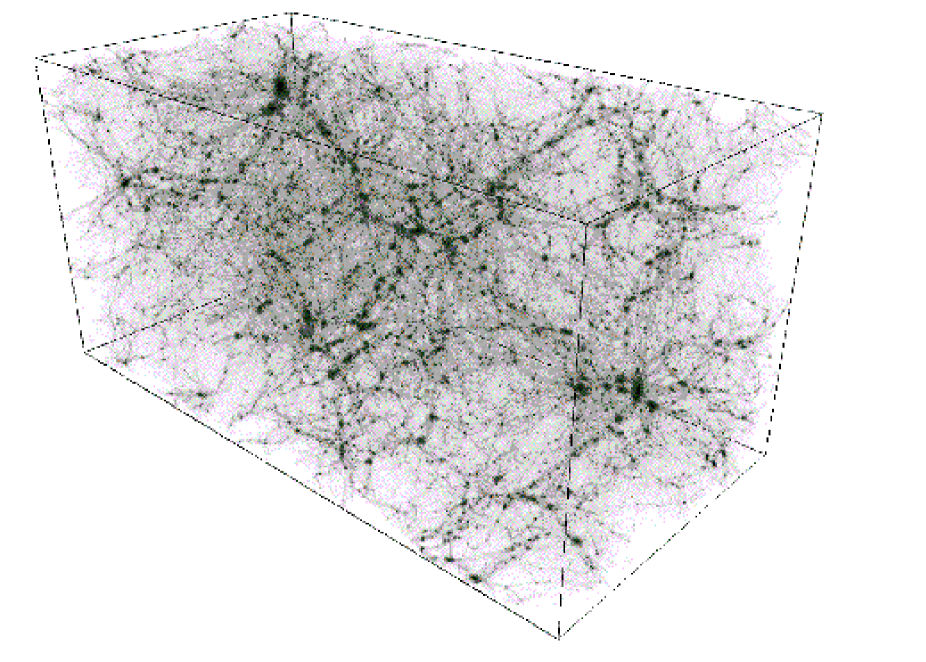
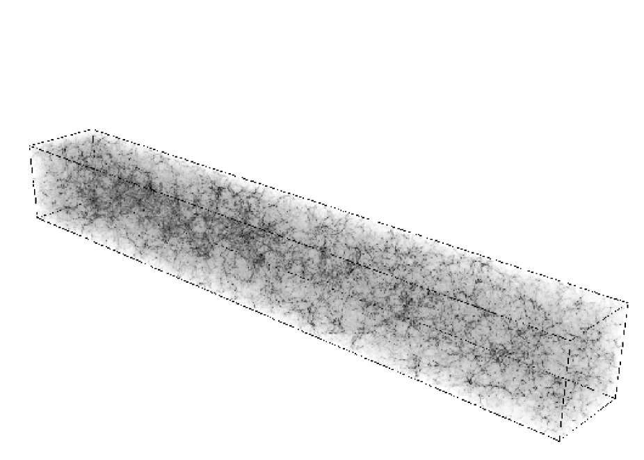
The simulations were run with a Particle-Mesh (PM) code, fully vectorized and parallelized on SGI-CRAY architecture with shared memory. The characteristics of the simulations, S and B, which involve respectively $\sim 32$ and $\sim 16$ millions particles, are given in Table 1. The cosmological parameters are inspired from Jenkins et al. (1998). The particles were laid down on a mesh with the same shape as the grid used to compute the forces. Then the Zel’dovich (1970) approximation was used to perturb the positions of the particles and to set up Gaussian initial conditions with the appropriate power-spectrum for standard Cold Dark Matter (CDM). This was done in a similar way as in the COSMICS package of Berstchinger (1995). To avoid effects of transients (e.g., Scoccimarro 1998), the simulations were started at high redshift $z=255$ and evolved until the desired redshift, $z=2$. Figs. 1 and  2 display the corresponding dark-matter distribution. A detailed analysis of the power-spectrum and the variance of the density field measured in the simulations is presented in appendix C.

The spatial comoving resolutions of simulations S and B are $\lambda_{\rm g}\simeq 4.9$ and $40$ km s^-1 respectively, which corresponds to physical resolutions $\sim 8.5$ and $68$ km s^-1 at $z=2$.

Table 1: Characteristics of the $N$-body experiments.

Model	$\Omega_{0}$	$\Lambda$	$h$	$\Gamma$	$\sigma_{8}$	$N_{\rm p}$	$L$
S	$1.0$	$0.0$	$0.5$	$0.5$	$0.51$	$512\times 256\times 256$	$50\times 25\times 25$
B	$1.0$	$0.0$	$0.5$	$0.5$	$0.51$	$1024\times 128\times 128$	$800\times 100\times 100$

Model: “S” and “B” stand for “small” and “big” respectively.

$\Omega_{0}$: value of the density parameter of the universe.

$\Lambda$: value of the cosmological constant.

$h$: parameterizes Hubble constant, $H_{0}=100h$ km/s/Mpc.

$\Gamma$: shape parameter of the initial power-spectrum (see, e.g., Jenkins et al. 1998 for details).

$\sigma_{8}^{2}$: the linear variance in the dark matter at present time in a sphere of radius $8h^{-1}$ Mpc (to fix the normalization).

$N_{\rm p}$: size of the grid used to compute the potential and the forces; also the number of particles.

$L$: dimensions of the rectangular periodic box in comoving Mpc.

This is to be compared with the maximum possible pixel resolutions of the instruments available on the VLT: UVES, $\lambda\simeq 3$ km/s, and FORS, $\lambda\simeq 100$ km/s. However, the actual resolution of the simulation depends on the physical parameter of interest and is always worse than the mesh resolution. For density related processes, we can expect the PM simulation to be sufficiently accurate at scales as small as $\sim 2\lambda_{\rm g}$, although dynamics can actually be contaminated by softening of the forces on scales as large as $6\lambda_{\rm g}$ (Bouchet et al. 1985). For velocities, which are quite sensitive to resolution, numerical comparisons between PM simulations and higher resolution codes show that results are correct within $\sim 25$ per cent at scales close to $\lambda_{\rm g}$ (e.g., Colombi 1996). Concerning the gas dynamics, density fluctuations are expected to be damped out below the Jeans length, and therefore it is not necessary to have a spatial resolution much better than this cut-off scale. For example, the thorough analysis of Gnedin & Hui (1998) shows that this scale is of the order of $50-100\,h^{-1}$ comoving kpc, i.e. $5-10$ comoving km s^-1. This roughly corresponds to the spatial resolution of the S simulation (at least for density-related quantities). In this respect, the resolution of the B simulation is not high enough, and this simulation is only used to test reconstruction of weakly non-linear structures.

In addition to small scale softening and limited resolution, discreteness effects represent another source of concern, particularly in under-dense regions. We apply adaptive Gaussian smoothing to the particle distribution as follows. The mean quadratic distance, $d_{i}$, between each particle, $i$, and its six nearest neighbours is computed. This sets a smoothing length, $\ell_{i}=d_{i}$, i.e. the Gaussian filter associated to particle $i$ is $W_{\ell_{i}}(r)\propto\exp(-r^{2}/2\ell_{i}^{2})$ within $3\ell_{i}$ after appropriate renormalization. In practice, the smoothed density (or mass weighted velocity) is computed on a grid chosen here to be the same as the simulation grid. Each cell, $j$, is subdivided in $N^{3}$ sub-pixels, $k_{j}$, corresponding to positions $x_{k_{j}}$, with $N=3$. The contribution of particle $i$ to the grid site $j$ writes

$$C_{j,i}\propto\sum_{{k_{j}},|r-x_{k_{j}}|\leq 3\ell_{i}}W_{\ell_{i}}(|r-x_{k_{j}}|),$$ (23)

with the appropriate normalization $\sum_{j}C_{j,i}=m_{i}$ where $m_{i}$ is the mass of particle $i$.

5 Application

In this section, we apply the methods discussed in § 3 to simulated Lyman $\alpha$ spectra extracted from the $N$-body simulations [using equation (6)].

Our preliminary analyses are organized as follows. In § 5.1, we give some details on the models and the priors used for both the Bayesian method and the constrained random field reconstruction. Section 5.2 deals with 3D reconstruction of the density field. We first test the constrained random field method in a régime where the density along each LOS  is supposed to be known. Next, we test the Bayesian approach. The latter method does not rely on such a strong prior for the density, and is first applied to the large scale régime discussed in § 2.2, where thermal broadening can be neglected. Moreover, redshift distortion is not taken into account. In section 5.3, we apply the Bayesian method to constrain the equation of state of the gas. We consider the small scale régime as discussed in § 2.2 but neglect redshift distortion again for the sake of simplicity, although peculiar velocity effects should realistically be accounted for. These velocities are dealt with in § 5.4, which assume in turn that the equation of state of the IGM is well constrained. We analyse the efficiency of velocity reconstruction versus number of LOSs, and test Bayesian reconstruction in the frameworks of strong and floating priors.

The reader will notice that for each problem considered, we neglect in turn either redshift distortion or thermal broadening. Accounting simultaneously for both effects can in principle be achieved with the explicit Bayesian method or a combination with the constrained random field reconstruction. However, our main goal here was to illustrate the method and to pin down various effects at each step of the reconstruction, concentrating on one particular property of the IGM, such as the structures of the 3D density field, the equation of state, or redshift distorsion. More general applications will be developed in future work.

Figure 3: Top panels, from left to right: The recovered log density versus the real (simulated) log density as a function of the distance between the LOSs, $L_{\rm LOS}$, as labeled: as expected the bias increases with $L_{\rm LOS}$; Middle panels, from left to right: the model and the reconstructed density for $L_{\rm LOS}=2.5,4$ and $5.5$ Mpc comoving; Bottom panels, from left to right: a slice of 1x80x80 Mpc across the simulation and the reconstructed fields (the scale on the panels is in pixels). Most of the small scale structures are lost in the reconstructed field. The large scale topology is however recovered. The rounded features in the reconstructed density are an artifact of the interpolation method.

5.1 The priors

5.1.1 Explicit Bayesian method

The Gaussian Bayesian prior [equation (10)] is fully described by the first two moments: the prior choice for the parameters of the model, ${\mathbf{M}}_{0}$, and its covariance, ${\mathbf{C}}_{0}$.

For the model we choose the following combination of fields and discrete parameters:

$${\mathbf{M}}=\left[\gamma(x,{\mathbf{x}}_{\perp}),v_{p}(x,{\mathbf{x}}_{\perp}),\overline{T},\beta\right]\,.$$ (24)

Function $\gamma(x,{\mathbf{x}}_{\perp})$ is defined as

$$\frac{\rho_{\rm DM}(x,{\mathbf{x}}_{\perp})}{{\overline{\rho}}_{\rm DM}}=D_{0}(x,{\mathbf{x}}_{\perp})\exp\left[\gamma(x,{\mathbf{x}}_{\perp})\right]\,,$$ (25)

so that positivity of density is insured. Here, $D_{0}(x,{\mathbf{x}}_{\perp})$ is an arbitrary function (specified later) which fixes the value of the prior for $\rho_{\rm DM}(x,{\mathbf{x}}_{\perp})/{\overline{\rho}}_{\rm DM}$, when $\gamma(x,{\mathbf{x}}_{\perp})=\gamma_{0}\equiv 0$. Note that $A(\overline{z})$ is assumed to be known throughout the paper.

For the prior, we take

$${\mathbf{M}}_{0}=\left[0,0,\overline{T}_{0},\beta_{0}\right]\,,$$ (26)

where the values of $\overline{T}_{0}$ and $\beta_{0}$ will be given in § 5.3.

We derive the prior covariance operator ${\mathbf{C}}_{0}$ either in an ad hoc manner (§ 5.2.2, 5.3 and 5.4.2) or from the simulations (§ 5.4.3). In the first case, ${\mathbf{C}}_{\gamma\gamma}$, is chosen to obey :

$${\mathbf{C}}_{\gamma\gamma}(x,x^{\prime},{\mathbf{x}}_{\perp},{\mathbf{x}}_{\perp}^{\prime})\equiv\sigma_{\gamma}^{2}\exp\left(-\frac{|x-x^{\prime}|}{\xi_{x}}\right)\exp\left(-\frac{|{\mathbf{x}}_{\perp}-{\mathbf{x}}_{\perp}^{\prime}|}{\xi_{T}}\right)\,,$$ (27)

where $\xi_{x}$ and $\xi_{T}$ are natural lengths in the inversion and govern the level of smoothness of the reconstruction. Typically, $\xi_{T}$ will be of order of the mean transverse distance between two lines of sight. The optimal choice for $\xi_{x}$ depends on the problem considered. If peculiar velocity effects are neglected, $\xi_{x}$ can be taken as small as the maximum scale between spectral resolution and Jeans length (§ 5.2.2 and § 5.3). In that case, no small scale information is lost along the LOSs. However, when redshift distortion is to be taken into account (e.g. § 5.4.2), it is necessary to have a smoother prior to stabilize the inversion, typically the length marking the transition toward the non-linear régime (in other words, the typical size of clumps).

The parameter $\sigma_{\gamma}$ may, if required, depend on position. On average, it corresponds roughly to the variance of $\gamma$ in a rectangle of volume $\xi_{x}\xi_{T}^{2}$. It governs indirectly by how much the reconstructed field, $\langle{\mathbf{M}}\rangle$, is allowed to float around the prior ${\mathbf{M}}_{0}$ while solving equation (11) with the iterative method detailed in Appendix A. When peculiar velocity effects are neglected, this parameter can be taken to be rather large, of the order of $0.2$. Otherwise, the inversion process is more complicated: details will be given in § 5.4.2. Exponential correlation functions turned out to be more appropriate than Gaussian ones in order to recover filamentary structures: the covariance kernel given in equation (27) is steeper, which allows us to take into account high density fluctuations.

5.1.2 Constrained random field reconstruction priors

The constrained random field reconstruction method, applied in § 5.2.1, § 5.4.1 and § 5.4.2, also requires values for the prior covariance matrix ${\mathbf{C}}_{0}$, which is taken to be those measured in the simulations, as detailed in Appendix B. Some of the biases involved in this choice are discussed in § 5.2.3.

5.2 Large scales structures: tomography of the IGM

We apply the two methods described in § 3 to recover the large scale structures in simulation B. For this purpose, we use a network of equally separated LOSs  along which we simulate spectra in accordance with equation (6) ( as shown in Fig. 5) while varying the separation. We proceed in two steps: we first ignore all issues related to finite signal to noise ratios, thermal broadening or line saturation, and use constrained random fields to extrapolate the density away from the LOSs  assuming that this latter is fully determined along the LOSs  (§ 5.2.1); we then illustrate the Bayesian technique, which does not suppose that the density along the LOSs  is known (§ 5.2.2). In the latter case, only the large scale régime is considered [i.e., the régime (ii) discussed in § 2.2] and redshift distortion is neglected ($v_{p}=0$). Section 5.2.3 discusses shortcomings of the two methods and realistic extensions.

5.2.1 Constrained random field

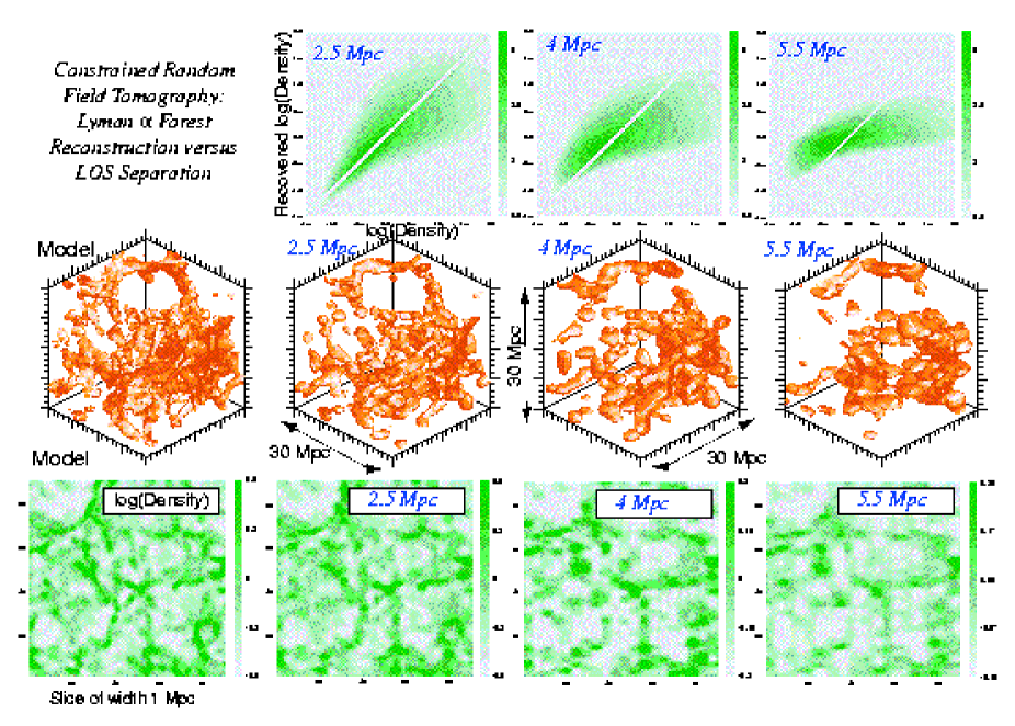
Let us first consider redshift space and assume that we have derived the density on each LOS  using for example equation (13). Recall that the most likely 3D density away from the lines of sight obeys equation (16). The covariance matrix of the prior, ${\mathbf{C}}_{0}={\mathbf{C}}_{\delta\delta}$, is shown on the top of the bottom right panel of Fig. 6. We present the results of a reconstruction of part of simulation B in Fig. 3. For this figure, we used the discrete form of equation (16), on a regular network of overlapping sub-grids of size $20\times 20\times 20$ pixels such that the centers of adjacent sub-grids are separated from each other by 10 pixels. The value of the reconstructed density on one pixel is obtained by a weighted interpolation of the recovered density on each sub-grid containing this pixel, the weight being inversely proportional to the distance of the pixel from the center of the sub-grid considered. This procedure insures smoothness of the reconstruction while keeping the size of the matrices reasonable. The top panels of Fig. 3 illustrate the bias in the extrapolation procedure as we vary the distances between LOSs, the middle panels display the 3D reconstructed iso-log densities corresponding to $\delta=0.2$, while the bottom panels show a slice through this field. The large scale filaments are recovered for all separations investigated, but small scale structures disappear beyond $2.5$ Mpc comoving of separation. The topography of the structures is well described. As expected the density is poorly recovered for the largest separations.

\begin{picture}(10.0,11.0)\centerline{\hbox{\mbox{\psfig{bbllx=50pt,bblly=35pt,bburx=560pt,bbury=757pt,angle=-90.0,width=455.24408pt}}}} \end{picture}

Figure 4: Density contrast reconstruction using the Bayesian algorithm from a set of 9$\times$9 lines of sight taken through simulation B. The distance between two adjacent lines of sight is equal to $2.4$ Mpc comoving. Each panel represents respectively on the left the reconstruction and on the right the simulation. Dark regions correspond to over-dense regions. The filaments are well recovered.

5.2.2 Bayesian reconstruction: line saturation and finite signal-to-noise ratio (SNR)

Choosing simply $D_{0}\equiv 1$ in equation (25), our model $g$, on pixelized data, reads [equation (8) with $v_{p}=0$, see also Appendix D.1.2]

$$g_{i\ell}(\gamma)=A(\overline{z})\exp[\alpha\gamma(w_{i\ell},x_{\perp\ell})]\,,$$ (28)

with $\alpha$ fixed equal to $1.7$ Here, $w_{i\ell}$ is the velocity at bin $i$ corresponding to the LOS  labelled $\ell$ and $\gamma(x,{\mathbf{x}}_{\perp})$ is the only parameter, for which the prior covariance is given by equation (27). The parameters $\sigma_{\gamma}$, $\xi_{x}$ are $\xi_{T}$ are respectively chosen equal to 1, twice the resolution and 1.5 times the distance between LOSs. The matrix ${\mathbf{G}}$ is given in Appendix D.1.2. Errors in the simulated data are modeled as follows. We assume that they are uncorrelated, so that the covariance error matrix ${\mathbf{C}}_{d}$ is diagonal, with elements given by

$$\sigma_{\tau}^{2}\equiv\frac{\sigma_{F}^{2}}{F^{2}}\simeq\frac{1}{(S/N)^{2}}+\frac{\sigma^{2}_{0}}{F^{2}}=\frac{1}{(S/N)^{2}}+{\sigma^{2}_{0}}\,{\exp(2\tau)}\,,$$ (29)

since the observed flux is simply: $F(w)=\exp\left({-\tau(w)}\right)$. Equation (29) states that the error on the flux has two origins: a constant signal to noise ratio component and a residual instrumental noise, $\sigma_{0}$, which dominates at large optical depth. In the inversion illustrated in Fig. 4, we use a SNR of 25 and a residual error of magnitude 0.01.

The reconstruction of filamentary structures is only effective in the régime where the distance between lines of sight is of the order of 1-3 Mpc comoving. Beyond this limit, the isotropic method presented here is insufficient to recover the structure of the IGM [such anisotropic features may be described by higher order correlation functions and stronger assumptions relying on a prior different from equation (10)]. Inherent to the method is the limitation that density fluctuations at scales smaller than the separation between LOSs  are damped out by the reconstruction. Also, the probability to intersect a given strong over-density is inversely proportional to the amplitude of the over-density. In other words the information regarding rare high over-densities is simply not sampled enough by the lines of sight. A related effect is induced by flux saturation in the spectra depending on the spectral resolution and the SNR. For instance optical depths of $\tau=5$ or $10$ will correspond to very different over-densities but very similar ($\approx 0$) fluxes. Note finally that for simplicity we have made use of Gaussian line profiles when Lorentzian would have been more appropriate.

5.2.3 Discussion

In the reconstruction of § 5.2.1, the density is assumed to be known along the LOSs, together with the covariance matrix of the 3D log-density field. At low spectral resolution, we may neglect both thermal broadening and peculiar velocities and use equation (13) to determine directly the density in redshift space from the Lyman-$\alpha$ forest along each LOS. At high spectral resolution, thermal debroadening and redshift distortion deconvolution could in principle be achieved simultaneously with the explicit Bayesian method or a combination of the Bayesian method with the constrained random field reconstruction, as discussed in § 3.2 and shown below.

Note also that our prior for the 3D covariance matrix in § 5.2.1 is optimal: it is measured directly in the simulation. In that sense, our reconstruction is biased since we use part of the correct answer in advance. Moreover, we go beyond Gaussian linear approximation, since we work on log-density, which contributes to improve even more the reconstruction. In real observations, we would not have a prior as good as that chosen here at our disposal. However, as shown in § 5.2.2, the results from the explicit Bayesian reconstruction, which rely on a much weaker prior, equation (27), give very similar results to the constrained random field reconstruction. This shows that the non linear features present in the measured correlations do not play an important role in our ability to carry out the inversion on the scales explored here. Finally, it may be worth mentioning again that the methods should be iterated, using for new priors and covariance matrixes the measured ones in the reconstructed field.

5.3 Small scales: the IGM temperature

Figure 5: Left panels: Inversion using different equations of state. The upper panel shows a portion of simulated spectrum through S. The equation of state used corresponds to equation (3) with $\bar{T}={\bar{T}}_{\rm t}\equiv 10^{4}\ K$, $\beta=\beta_{\rm t}\equiv 0.2$. Peculiar velocities are not considered. The lower panel shows the simulated density as black dots. The density recovered using the same equation of state is plotted as a solid line; it is apparent that even the internal structure of absorption blends is recovered. Other curves correspond to the results of inversions using various lower values of $\bar{T}$ at fixed $\beta=0.2$. The effect of lowering $\bar{T}$ is to give smaller values for reconstructed density with a reduced $\chi^{2}<1$. If, on the contrary, ${\bar{T}}>T_{\rm t}$, one obtains $\chi^{2}\gg 1$. Right panel: Map of convergence ($\chi^{2}<1$) or divergence ($\chi^{2}\gg 1$) for inversions using equation (30) with different values of ${\bar{T}}$ and $\beta$. The LOS  is the same as in left panels.

We now aim to determine the equation of state of the IGM by considering the inversion of a single LOS  observed at high spectral resolution [régime (i) in § 2.2]. The inversion of the density, velocity and temperature fields from a single LOS  is not unique (Theuns et al. 1999a; Hui & Rutledge 1999). Indeed, the same spectrum can be reconstructed with different equations of state and density distributions as illustrated by Fig. 5. Neglecting peculiar velocities for the sake of simplicity ($v_{p}=0$), the problem reduces to the determination of two parameters $\bar{T}$ and $\beta$ and one unknown field, $\gamma$. The simultaneous determination of these parameters and the field remains a degenerate problem. As detailed in appendix D.1.1, our model, $g$, on pixelized data reads, from equation (6),

$$g_{i\ell}(\gamma)=A(\overline{z})c_{1}\int\!\!\!\!\!\int\left(\int_{-\infty}^{+\infty}(D_{0}(x,{\mathbf{x}}_{\perp})\exp[\gamma(x,{\mathbf{x}}_{\perp})])^{\alpha-\beta}\exp\left(-c_{2}\frac{(w_{i\ell}-x)^{2}}{(D_{0}(x,{\mathbf{x}}_{\perp})\exp[\gamma(x,{\mathbf{x}}_{\perp})])^{2\beta}}\right){{\mathrm{d}}{x}}\right)\delta_{D}({\mathbf{x}}_{\perp}-x_{\perp\ell}){{\mathrm{d}}{}}^{2}{\mathbf{x}}_{\perp}.$$ (30)

Here, $A({\bar{z}})$ is arbitrarily fixed to $A({\bar{z}})=0.7$ as explained in § 5.1.1, $\alpha=2-1.4\beta$ [equation (4)] and $c_{1}$ and $c_{2}$ are functions of $\bar{T}$ [equation (7)]. The function $D_{0}(x,{\mathbf{x}}_{\perp})$ is chosen to be

$$D_{0}(x,x_{\perp})=\left(\frac{\tau_{\ell}(w\equiv x)}{A(\overline{z})}\right)^{1/\alpha}\,.$$ (31)

The prior covariance matrix $C_{\gamma\gamma}$ is given by equation (27) with $\xi_{T}\rightarrow\infty$. Here $\xi_{x}$ and $\sigma_{\gamma}$ are chosen equal to 0.2 Mpc comoving and 0.2.

We conduct our analyses as follows. We first simulate a spectrum along one LOS with a given real pair ($\beta_{\rm t}$, $\bar{T}_{\rm t}$). The noise matrix ${\mathbf{C}}_{d}$ is the same as in § 5.2.2 with a $(S/N,\sigma_{0})=(50,0.05)$. We then invert this LOS  for $\gamma(x)$ while varying ($\beta$, $\bar{T}$) over a given range of realistic values. In that sense, the only effective parameter in the inversion is the field $\gamma$. For each value of $(\beta,{\bar{T}})$, we compute the reduced $\chi^{2}$, i.e. $({\mathbf{D}}-g({\mathbf{M}}))^{\perp}.{\mathbf{C}}_{d}^{-1}.({\mathbf{D}}-g({\mathbf{M}}))$ in equation (10), as shown in right panel of Fig. 5. The value of ($\beta_{\rm t}$, $\bar{T}_{\rm t}$) is shown by a white cross. The ($\beta$, $\bar{T}$) plane is divided into two regions separated by a straight borderline, one with $\chi^{2}\gg 1$ (corresponding to large values of ${\bar{T}}$) and the other one with $\chi^{2}\leq 1$. This arises because the absorption lines are indeed thermally broadened and resolved. When ${\bar{T}}>{\bar{T}}_{\rm t}$, the absorption features in the data are narrower than the model and cannot be fitted anymore.

As expected, the real parameters stand on the borderline between convergence and divergence: these parameters correspond to a good fit. We cannot however distinguish –using a $\chi^{2}$ criterion– between pairs of $(\beta,{\bar{T}})$ on this borderline. Even though the degeneracy is not completely lifted, this analysis provides a complementary method to the standard techniques of Voigh profile fitting (see Ricotti et al. 2000; Schaye et al. 1999) to measure the mean properties of the IGM and its cosmological evolution. The application of our method to real data is developed to a companion paper (Rollinde, Petitjean & Pichon, submitted).

Note finally that, for close enough lines of sight (e.g. multiple lensed QSO images) we might in theory be able to investigate the small scale 3D properties of the IGM while accounting for thermal broadening.

Figure 6: Left panel: the 3D correlation function, ${\mathbf{C}}_{v\delta}(x,{\mathbf{x}}_{\perp})$, measured in simulation S. Top right panel: the filter $K^{(v)}$ required to compute the most likely velocities along one LOS  [equation (14) with $\ell=\ell^{\prime}=L=1$]. The width of the filter shows that the peculiar velocity has two natural scales as discussed in the main text. Bottom right panel: the 1D LOS  correlation functions: top sub-panel: $\log({\mathbf{C}}_{\delta\delta})$ ; middle sub-panel: ${\mathbf{C}}_{vv}$; bottom sub-panel: ${\mathbf{C}}_{\delta v}$.

5.4 Redshift distortion

Recall that in this section, for the sake of simplicity, we assume that the equation of state of the IGM is known.

There are several issues to address here. The optical depth along a bundle of LOSs  does not constrain uniquely the corresponding velocity field. This would require the knowledge of the full 3D density distribution together with the assumption that linear dynamic applies. Thus, we first investigate how increasing the number of measured LOSs  or changing the mean separation between them improves the likelihood of the corresponding realization of the constrained velocity field for a given density field along the bundle (§ 5.4.1). We then turn to the problem of deconvolving the optical depth in real space, but conduct a preliminary analysis on a single LOS. We test two approaches. The first approach is a strong prior inversion (§ 5.4.2), i.e. it relies on the Bayesian formalism while assuming that the velocity field takes its most likely value. The second method allows the velocity field to float around this most likely value (§ 5.4.3). Finally, we discuss the limitations of the present work and possible improvements (§ 5.4.4).

Let us briefly describe the filters and correlation function involved. Fig. 6 (left panel) displays the 3D correlation function, ${\mathbf{C}}_{v\delta}(x,{\mathbf{x}}_{\perp})$, measured in simulation S. It is antisymmetric along the LOS, and symmetric orthogonally. The top right panel shows the 1D filter, $K^{(v)}(x,y)$ [equation (14) with $\ell=\ell^{\prime}=L=1$], which was in practice computed according to the prescription sketched in Appendix B. This antisymmetric filter presents two characteristic scales: a strong peak at $\approx 2$ Mpc (comoving) and broad wings up to $\approx 20$ Mpc. This implies that the most likely velocity at a given point will depend on the local density and also significantly on the density further away (up to $\approx 20$ Mpc). Transversally the shape of the 3D cross correlation function, ${\mathbf{C}}_{v\delta}(x,{\mathbf{x}}_{\perp})$, which vanishes near the line ${x}=0$, implies that the density away from a given point will dominate the local velocity field.

5.4.1 Most likely velocity versus LOS  separation & number of LOSs

In this subsection we assume temporarily that the log-density field is known along a bundle of LOSs. In the framework of constrained random field (§ 3.2), equation (14) gives the relationship between the most likely velocity along a given bundle of LOSs  and the corresponding log-density.

Let us define the quality factor, $Q$, as

$$Q\equiv\frac{\sigma_{v_{p}}}{\sigma_{\delta v_{p}}}=\sqrt{\frac{\langle v_{p}^{2}\rangle}{\left\langle\left(v_{p}-v_{\rm rec}\right)^{2}\right\rangle}}\,,$$ (32)

where $v_{\rm rec}$ is the reconstructed velocity. Parameter $Q$ measures the inverse residual misfit in units of the variance for the velocity. We show in Fig. 7 (top left panel) that this number increases with the number of LOSs  sampling the sky, as expected. However, $Q$ increases as well with the distance between LOSs  until it reaches a maximum, which might sound confusing. This can be easily understood by examining left panel of Fig. 6. In fact, a bundle of LOSs  constrains the transverse 3D velocity distribution at intermediate scales, as a result of a competition between short range and long range correlations:

1. High frequency structures are read from the LOS  through the two strong peaks along the x coordinate axis on the left panel of Fig. 6 (at approximately $\pm 0.8$ Mpc). Other LOSs  can in principle contribute to small scales, but only if they are found very close to the LOS  of interest (i.e. with ${\mathbf{x}}_{\perp}\simeq 0$).

2. Low 3D frequency features are mainly sampled by LOSs  away from the LOS  of interest, due to the significant tails present on ${\mathbf{C}}_{v\delta}$ at scales as large as $\sim$ 20 Mpc, as illustrated by top right panel of Fig. 6. This effect is three-dimensional, i.e. in all directions: it thus provides information on the structures transverse to the LOS.

(Note that in this discussion, we implicitly assumed that ${\mathbf{C}}_{\delta\delta}\simeq$ identity in equation (14). Taking into account the real contribution of matrix ${\mathbf{C}}_{\delta\delta}^{-1}$ would simply boil down to smoothing the density with an isotropic filter, which has no effect on our qualitatives conclusions).

The competition between effects (i) and (ii) fixes an optimal separation between the LOSs  as a function of their number. From the top left panel of Fig. 7, we see for example that the optimal separation is $5$ Mpc for a bundle of 11$\times$ 11 LOSs. For a bundle with a smaller number of LOSs, the optimal separation becomes larger so that the tails of ${\mathbf{C}}_{v\delta}$ are still fully sampled (but with a sparser binning and thus a smaller quality factor).

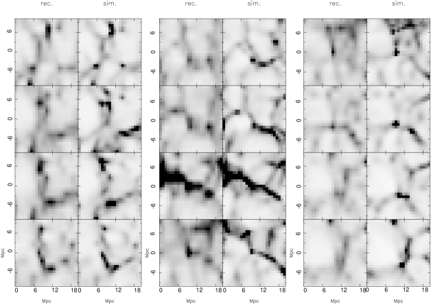
The bottom right and left panels of Fig. 7 compare the velocity along one LOS  measured in the simulation to the reconstructed one by applying equation (14) to bundles of various sizes (1$\times$1, 5$\times$5 and 11$\times$11) distributed uniformly on the sky (from simulation B), with a mean separation of $2.5$ Mpc. With only one LOS, the reconstructed velocity does not account in detail for small structures although it seems to match well large scale flows in the example studied here. Increasing the number of LOSs  significantly improves the reconstruction: with a bundle of 11$\times$11 LOSs, the reconstruction almost perfectly matches the simulation.

An important outcome of this analysis is that since the optimal separation between LOSs  is rather large (a few Mpc), the small scale information in the reconstruction is only contained in the LOS  of interest. Therefore, having high resolution spectra on all the LOSs  is not required: a survey dedicated to real space reconstruction should provide a high resolution spectrum together with a set of low resolution spectra separated by distances smaller than or of the order of $\approx 4-5$ Mpc comoving. Note that $Q$ was computed while averaging over the whole bundle: the quality of the reconstruction in fact depends on the position of the LOS  in the bundle, as illustrated in the top right panel of Fig. 7. Obviously, the quality factor is optimal at the center of the bundle: the high resolution spectrum should be located there.

Figure 7: Top left panel: quality of the reconstruction [equation (32)] versus LOS  separation and number of LOSs. Increasing the sampling on the sky decreases the dispersion between the constrained most likely velocity and the measured velocity as discussed in the text. Note the saturation for 11$\times$11 LOSs  at a separation of $\simeq$ 5 Mpc. Top right panel: isocontour for the quality of the reconstruction projected on the sky for a bundle of $11\times 11$ LOSs, separated by $2.4$ Mpc comoving. Note that the reconstruction obviously works better for the central LOSs. Bottom left panel: in simulation B, most likely velocity constrained by a single LOS. The solid line on the upper sub-panel corresponds to simulated velocity and the dashed one to the reconstructed velocity. The simulated density is displayed on lower sub-panel. Bottom right panel: solid lines: simulated velocities along the center of a bundle of $5\times 5$ LOSs  or $11\times 11$ LOSs; dashed lines: corresponding recovered velocities.

We assumed here the 3D covariance matrices needed for the reconstruction were known. In fact, we used the best possible guess for them since they were derived from direct measurement in the simulation. In reality we would have to proceed iteratively: for a given power spectrum, we could recover the 3D density, compute perturbatively the corresponding 3D velocity field and derive a new covariance matrix until convergence is achieved. We have not demonstrated here that this procedure is convergent. This is certainly a possible shortcoming of the procedure.

5.4.2 Strong prior inversion

Let us now try to deconvolve the density in real space along one LOS. A combination of the general Bayesian method and the constrained random field technique is implemented: the constrained random field method allows us to relate the unknown field $v_{p}$ to $\gamma$, imposing that the peculiar velocity takes its most likely value, but the recovery of $\gamma$ is still based on the Bayesian method. Our model, $g_{i}(\gamma)$, is now :

$$g_{i}(\gamma)=A(\overline{z})c_{1}\int_{-\infty}^{+\infty}(D_{0}(x)\exp[\gamma(x)])^{\alpha-\beta}\exp\left(-c_{2}\frac{(w_{i}-x-v_{p}(x))^{2}}{(D_{0}(x)\exp[\gamma(x)])^{2\beta}}\right)\,{{\mathrm{d}}{x}}\,,$$ (33)

with the supplementary assumption that the peculiar velocity in equation (33) equals the most likely velocity (Appendix B):

$$v_{p}(x)=\langle v\rangle\equiv\int K^{(v)}(x,y)\gamma{(y)}{{\mathrm{d}}{y}}\,,\quad\mbox{ where }\quad K^{(v)}(x,y)\equiv\frac{1}{2\pi}\int e^{ik_{x}(x-y)}\,\frac{P_{v\delta,{\rm 1D}}(k_{x})}{P_{\delta\delta,{\rm 1D}}(k_{x})}{{\mathrm{d}}{k}}_{x}\,.$$ (34)

The unknown parameter remains the density contrast. The prior for the density is chosen as $D_{0}\equiv 1$ so that $\gamma=\delta$. For the filter $K^{(v)}(x,y)$ we use a simple analytic fit of the function $K^{(v)}(x,y)$ measured in the simulation as explained in Appendix B.1.1. The derivation of the different vectors and matrixes involved in this case is sketched in Appendix D.2.1. The practicalities involves fixing appropriately the parameters $(\sigma_{\gamma},\xi_{x})$ in equation (27) ($\xi_{T}\equiv\infty$ for a single LOS) for the minimization procedure detailed in Appendix A to converge while providing as accurate reconstruction as possible. To stabilize the inversion, we need to take for $\xi_{x}$ a value close to the correlation length, $\xi_{x}=1$ Mpc. With a larger value of $\xi_{x}$, the inversion is still stable but makes the reconstructed density field too smooth, while a smaller value of $\xi_{x}$ makes the inversion unstable. The choice of $\sigma_{\gamma}$, which fixes the amount of variations allowed around the prior, is more delicate. A small value of $\sigma_{\gamma}$ makes convergence easier, but does not leave enough freedom for the reconstructed density to float around the prior: voids tend to be filled, and high density peaks are not saturated. On the contrary, a large value for $\sigma_{\gamma}$ allows significant deviations from the prior but makes the iteration procedure less stable. For this reason, the reconstruction is carried in two steps. We first take a small value for $\sigma_{\gamma}=0.0175$, and reconstruct the density while using equation (34) to determine accurately the most likely velocity. Because of our choice of $\sigma_{\gamma}$, the reconstructed density is not as contrasted as it should be, but this does not affect significantly the corresponding most likely velocity: it just makes it smoother. In the second step, we fix the most likely velocity at the value obtained from the first step. Thus equation (34) is disregarded, and we iterate once more on the density with a larger value of $\sigma_{\gamma}$, $\sigma_{\gamma}=0.2$, allowing more variations of the density around the new prior –the reconstructed density obtained from the first step. The fact that the most likely velocity is fixed indeed makes the inversion more stable and allows larger values of $\sigma_{\gamma}$.

Fig. 7 illustrates how the method performs on two unsaturated LOSs: the first isolated and the latter nearby a cluster. The simulated spectra assume $A=0.39$, $\beta=0.4$, ${\bar{T}}=10^{4}$ K, and were calculated after smoothing the density and velocity fields with a cube of size $\sim 200$ kpc (2 cells). The errors in the data are modelled as described in § 5.2.2 with $(S/N,\sigma_{0})=(100,0.05)$ in equation (29). As expected, the reconstructed velocity matchs the original only when there is no significant structure close to the LOS, likely to induce large-scale infall contamination. Bottom panels of Fig. 7 show that the reconstructed density reproduces well the shape of most structures, except that they are not correctly located along the velocity axis on bottom right panel.

Note that our two-step procedure is similar in spirit to that proposed by Nusser & Haehnelt (1999a), although we use same smoothing length $\xi_{x}$ in both steps, which allows more small scale features on the reconstructed density. Also, our method is not yet able to deal with spectra containing significantly saturated absorption lines: in that case, the inversion is much less stable and the reconstructed most likely velocity is often unrealistic, even if the LOS  is isolated. Finally, we assumed the kernel function $K^{(v)}(x,y)$ was known, which should not be the case in reality: a more detailed study of the effects of the assumed shape for this function will be needed in the future to fully qualify the method.

5.4.3 Floating prior for the velocities.

A less biased representation of the underlying field would be to assume that $\gamma$ and $v_{p}$ are two fields which are statistically correlated (by the dynamics) but whose realizations are independent. The model is formally identical to equation (33) with the restriction that $v_{p}$ does not obey equation (34) anymore. The vector of the model parameters is : ${\mathbf{M}}=\left(\gamma(x),v_{p}(x)\right)$. The correlation between $\gamma$ and $v_{p}$, ${\mathbf{C}}_{v\gamma}$, is considered to be linear. Recall that the prior variance-covariance matrix, ${\mathbf{C}}_{0}$, has three independent terms, shown in bottom right panel of Fig. 6:

$${\mathbf{C}}_{0}=\left(\begin{array}[]{cc}{\mathbf{C}}_{\gamma\gamma}&{\mathbf{C}}_{v\gamma}\\ {{{\mathbf{C}}_{v\gamma}}^{\bot}}&{\mathbf{C}}_{vv}\\ \end{array}\right)\,.$$ (35)

The penalty function then obeys equation (22), and realizations of the velocity field are entitled to float around their most likely values, equation (14). The corresponding model, $g$, is sketched in Appendix D.2.2. The iterative procedure presented in Appendix A brings the reduced $\chi^{2}$ down from values of about a $100$ to $1\pm\sqrt{2/N}$ in a few iterations, but does not converge if peculiar velocities induce displacements larger than the effective width of the absorption lines. Even though the weak prior inversion is more elegant and easier to implement than the strong prior approach (cf. Appendix D.2.2), it seems to fail to constrain sufficiently our model when redshift distortion is important. This arises because the effective correlation in equation (22) is too weak to induce convergence.

5.4.4 Discussion

A priori, the best approach for reconstructing the density in redshift space would be to use the explicit Bayesian method with a floating prior for the velocity described in § 5.4.3. However, our preliminary analyses show that this method fails to converge when applied to one LOS  if redshift distortion becomes of the order of the width of absorption lines, which is unfortunately the case in realistic situations. The strong prior inversion of § 5.4.2, tested again on one LOS, seems to be more reliable, but gives accurate reconstruction only if the considered LOS  is unsaturated and is isolated from large structures. The only reliable way to improve the reconstruction is therefore to have more information on the 3D structure of the intergalactic medium through bundles of LOSs, as studied in § 5.4.1. The diference between § 5.4.3 and § 5.4.2 would then vanish, since the discrepency between the most likely velocity and the actual field becomes smaller and smaller, while the correlation between the density and the velocity becomes simultaneously tighter and tighter. However, we have not explicitely tested the methods of § 5.4.2 and § 5.4.3 on several LOSs : this is left for future work.

Figure 8: Inversion while accounting for peculiar velocity with strong prior. Simulation S is used to test the method. Two examples are considered, according to whether there is a large structure nearby the LOS  or not (respectively right and left panels). Top panels: the simulated spectra. Middle panels: the simulated (solid line) and most likely (dotted line) peculiar velocity along the LOS. Bottom panels: the simulation (solid line) and reconstructed (dotted line) log-density (in $\log_{10}$ units).

6 Conclusion

In this paper, an explicit Bayesian technique and a constrained random field method have been proposed to recover various properties of the intergalactic medium from observations of the Lyman-$\alpha$ forest along LOSs  to quasars. In particular, our preliminary analyses suggest that these methods may be used (i) to recover the large scale 3D topology of the IGM from inversion of a network of adjacent LOSs  observed at low spectral resolution; (ii) to constrain the physical characteristics of the gas from inversion of single LOSs  observed at high spectral resolution; (iii) to investigate how the number of and the distance between LOSs  constrain the projected peculiar velocities; (iv) to correct in part for redshift distortions induced by these velocities using either strong or weak priors.

Both approaches rely on prior assumptions on the covariance of the log-density field and the cross-correlation between the log-density field and the peculiar velocity field.

These methods are used in various régimes: as extrapolation tools to recover the 3D structure of the IGM; as non-linear deconvolution tools to correct for blending; as non-parametric field extractors and as model fitting routines to constrain the parameters of the equation of state.

We have demonstrated (§ 3.3) that as far as extrapolation is concerned the standard constrained random field interpolation scheme could be viewed as a specific linear sub-case of the Bayesian inversion scheme presented in § 3.1. The method presented in § 3.1 is therefore complementary to, and more general than standard constrained random field techniques: it can also cope with thermal broadening and finite signal to noise, in a manner similar to Wiener filtering, but allows for non-linear models and non-zero mean priors. The correlation functions required for the prior need not be measured in the simulations, and can be postulated. It is more flexible since some level of redshift distortion can in principle be corrected for using the full 3D information along the bundle (although we did not demonstrate it explicitly in this paper). It is well suited for this kind of problems since it deals directly with unknown continuous fields [i.e. the parameter space is the Hilbert space L2; see, e.g. equation (75)]. In contrast with the Lucy-Richardson algorithm, regularization is built in.

We have shown that temperature inversion is degenerate with respect to two parameters describing the equation of state of the gas, the temperature scale factor, $\bar{T}$ and the effective polytropic index $\beta$.

Recall that we have assumed in this paper the correlation matrices of the log density to be fixed a priori, together with the cross-correlation of the log density and the velocities when dealing with peculiar velocities. When the method is applied to real data, we will proceed iteratively and recompute these (cross-) correlations once the 3D reconstruction is achieved. We expect this procedure to converge and that the convergence limit will not depend too strongly on the initial prior.

A thorough analysis of the various biases involved in the methods presented here is postponed to a companion paper which will investigate statistically the properties of the reconstructed fields and the degeneracies involved in recovering the density and the temperature while relying on numerical hydrodynamical simulations. Since this inversion method relies on existing cross correlation between the density and the velocity fields, it should still be applicable on scales where dark matter dynamics is less relevant, so long as such correlations exist. We have left aside for now the simultaneous true 3D deconvolution of both the temperature and the peculiar velocities.

Appendix A Minimization procedure.

In this section we sketch an iterative procedure leading to the optimization of the posterior probability of the model for a given data set in equation (10). The minimum of the argument of the exponential in equation (10) is shown by a simple variational argument (Tarantola and Valette, 1982a; 1982b) to obey the implicit equation:

$$\langle{{\mathbf{M}}}\rangle={\mathbf{M}}_{0}+{\mathbf{C}}_{0}\cdot{{{\mathbf{G}}}^{\bot}}\cdot({\mathbf{C}}_{d}+{\mathbf{G}}\cdot{\mathbf{C}}_{0}\cdot{{{\mathbf{G}}}^{\bot}})^{-1}\cdot({\mathbf{D}}+{\mathbf{G}}\cdot(\langle{{\mathbf{M}}}\rangle-{\mathbf{M}}_{0})-g(\langle{{\mathbf{M}}}\rangle))\,,$$ (36)

with ${\mathbf{G}}$, the matrix of partial derivatives:

$${\mathbf{G}}=\left(\frac{\partial g}{\partial{\mathbf{M}}}\right)\,.$$ (37)

This minimum is found using an iterative procedure:

$${{\mathbf{M}}}_{[k+1]}={\mathbf{M}}_{0}+{\mathbf{C}}_{0}\cdot{{{\mathbf{G}}_{[k]}}^{\bot}}\cdot({\mathbf{C}}_{d}+{\mathbf{G}}_{[k]}\cdot{\mathbf{C}}_{0}\cdot{{{\mathbf{G}}_{[k]}}^{\bot}})^{-1}\cdot({\mathbf{D}}+{\mathbf{G}}_{[k]}\cdot({{\mathbf{M}}}_{[k]}-{\mathbf{M}}_{0})-g({{\mathbf{M}}}_{[k]}))\,,$$ (38)

where subscript $[k]$ refers to the iteration order. In this scheme the minimum corresponds to ${\tilde{\mathbf{M}}}={\mathbf{M}}_{[\infty]}$ and in practice is found via a convergence criterion on the relative changes between iteration $[k]$ and $[k+1]$. For the sake of numerical efficiency, rather than inverting $({\mathbf{C}}_{d}+{\mathbf{G}}_{[k]}\cdot{\mathbf{C}}_{0}\cdot{{{\mathbf{G}}_{[k]}}^{\bot}})$, we solve for the vector ${\mathbf{W}}_{[k]}$ satisfying

$${\mathbf{S}}_{[k]}\cdot{\mathbf{W}}_{[k]}=({\mathbf{D}}+{\mathbf{G}}_{[k]}\cdot({{\mathbf{M}}}_{[k]}-{\mathbf{M}}_{0})-g({{\mathbf{M}}}_{[k]})),\quad{\rm where}\quad{\mathbf{S}}_{[k]}={\mathbf{C}}_{d}+{\mathbf{G}}_{[k]}\cdot{\mathbf{C}}_{0}\cdot{{{\mathbf{G}}_{[k]}}^{\bot}}\,,$$ (39)

and iterate:

$${{\mathbf{M}}}_{[k+1]}={\mathbf{M}}_{0}+{\mathbf{C}}_{0}\cdot{{{\mathbf{G}}_{[k]}}^{\bot}}\cdot{\mathbf{W}}_{[k]}\,.$$ (40)

From now on, we drop the subscript $[k]$. Once the maximum of equation (10) has been reached, an approximation of the internal error made on the parameter estimation is derived from a second order development of the posterior distribution function in the vicinity of the solution :

$${\mathbf{C}}_{{{\mathbf{M}}}}={\mathbf{C}}_{0}-{\mathbf{C}}_{0}\cdot{{{\mathbf{G}}}^{\bot}}\cdot{\mathbf{S}}^{-1}\cdot{\mathbf{G}}\cdot{\mathbf{C}}_{0}\,.$$ (41)

The high spatial frequency fluctuations are lost in the inverse process because of limited resolution and finite signal to noise ratio. The prior correlation function therefore plays an important role to transform an ill-posed problem into an invertible one. How is the density information degraded in the spectra? This question can be addressed via the resolving kernel, ${\mathbf{R}}$, introduced for the first time by Backus and Gilbert (1970) and which gives the spread of the density estimation at a given position. Suppose that we know the true model, ${\mathbf{M}}_{\rm true}$. The data can be written: ${\mathbf{D}}={\mathbf{g}}({\mathbf{M}}_{\rm true})\,$. Approximating locally operator $g$ near its minimum as a linear operator, equation (36) yields:

$$\langle{{\mathbf{M}}}\rangle-{\mathbf{M}}_{0}={\mathbf{C}}_{0}\cdot{{{\mathbf{G}}}^{\bot}}\cdot{\mathbf{S}}^{-1}\cdot{\mathbf{G}}\cdot({\mathbf{M}}_{\rm true}-{\mathbf{M}}_{0})\equiv{\mathbf{R}}\cdot({\mathbf{M}}_{\rm true}-{\mathbf{M}}_{0})\,,$$ (42)

which defines the resolving kernel ${\mathbf{R}}(x,x^{\prime})$ as a low band pass filter.

Appendix B Constraints random fields & Multiple line of sights

As a though experiment, let us assume that we know the density contrast $\delta$ on n points and ask what the corresponding most likely velocity (or density) at points labeled $k=1\cdots p$, $\varpi_{k}$ is. We shall not assume that the densities $\delta_{1},\cdots,\delta_{n}$ are necessarily along the same LOS  nor that the quantity $\varpi_{k}$ is sought along any of these. Let $X=[{\varpi_{1},\cdots,\varpi_{p},\delta_{1},\cdots,\delta_{n}}]$. We define

$${\mathbf{C}}\equiv\left[{\matrix{\langle{\varpi_{1}}{\varpi_{1}}\rangle&\cdots&\langle{\varpi_{1}}{\varpi_{p}}\rangle&\langle{\varpi_{1}}{{\delta}_{1}}\rangle&\cdots&\langle{\varpi_{1}}{{\delta}_{n}}\rangle\cr\vdots&\ddots&\vdots&\vdots&\ddots&\vdots\cr\langle{\varpi_{1}}{\varpi_{p}}\rangle&\cdots&\langle{\varpi_{p}}{\varpi_{p}}\rangle&\langle{\varpi_{p}}{{\delta}_{1}}\rangle&\cdots&\langle{\varpi_{p}}{{\delta}_{n}}\rangle\cr\langle{\varpi_{1}}{{\delta}_{1}}\rangle&\cdots&\langle{\varpi_{p}}{{\delta}_{1}}\rangle&\langle{{\delta}_{1}}{{\delta}_{1}}\rangle&\cdots&\langle{{\delta}_{1}}{{\delta}_{n}}\rangle\cr\vdots&\ddots&\vdots&\vdots&\ddots&\vdots\cr\langle{\varpi_{1}}{{\delta}_{n}}\rangle&\cdots&\langle{\varpi_{p}}{{\delta}_{n}}\rangle&\langle{{\delta}_{1}}{{\delta}_{n}}\rangle&\cdots&\langle{{\delta}_{n}}{{\delta}_{n}}\rangle}}\right]\equiv{\left[\begin{array}[]{cc}{\mathbf{C}}_{ww}&{\mathbf{C}}_{w\delta}\\ {{\mathbf{C}}}^{\perp}_{w\delta}&{\mathbf{C}}_{\delta\delta}\end{array}\right]}\,,$$ (43)

so that ${\mathbf{C}}_{ww}$ is the $p\times p$ autocorrelation matrix of the sought field, ${\mathbf{C}}_{\delta\delta}$ is the $n\times n$ autocorrelation matrix of the known density field, and ${\mathbf{C}}_{w\delta}$ is the $p\times n$ cross-correlation matrix of the sought field with the density field. The joint probability of achieving velocity $\varpi_{k}$ and density profile $\delta_{1},\cdots,\delta_{n}$ is given by

$$p({\mathbf{X}}){{\mathrm{d}}{}}^{n+p}X=p(\varpi_{1},\cdots,\varpi_{p},\delta_{1},\cdots,\delta_{n}){{\mathrm{d}}{\varpi_{1}}}\cdots{{\mathrm{d}}{\varpi_{p}}}{{\mathrm{d}}{\delta}}_{1}\cdots{{\mathrm{d}}{\delta}}_{n}=\exp\left[{-{1\over 2}\left\{{\sum\limits_{a,b=1\cdots n+p}{\left({C^{-1}}\right)_{a,b}X_{a}X_{b}}}\right\}}\right]\,\frac{{{\mathrm{d}}{}}^{n+p}X}{\sqrt{(2\pi)^{n+p}\rm{det}{|C|}}}\,.$$

The argument of the exponential can be rearranged as

$${{{\left({\mbox{\boldmath$\varpi$}},{\mathbf{\delta}}\right)}^{\bot}}}\cdot{{\left[\begin{array}[]{cc}{\mathbf{C}}_{ww}&{\mathbf{C}}_{w\delta}\\ {{\mathbf{C}}}^{\perp}_{w\delta}&{\mathbf{C}}_{\delta\delta}\end{array}\right]}^{-1}}\cdot\left({\mbox{\boldmath$\varpi$}},{\mathbf{\delta}}\right)={{{\left({\mbox{\boldmath$\varpi$}}-{\mathbf{C}}_{w\delta}\cdot{{\mathbf{C}}_{\delta\delta}^{-1}}\cdot{\mathbf{\delta}}\right)}^{\bot}}}\cdot{{\left({\mathbf{C}}_{ww}-{{\mathbf{C}}_{w\delta}}\cdot{{\mathbf{C}}_{\delta\delta}^{-1}}\cdot{{{\mathbf{C}}_{w\delta}}^{\bot}}\right)^{-1}}\cdot\left({\mbox{\boldmath$\varpi$}}-{\mathbf{C}}_{w\delta}\cdot{{\mathbf{C}}_{\delta\delta}^{-1}}\cdot{\mathbf{\delta}}\right)}+\quad{\rm rest}$$ (44)

where “rest” stands for terms independent of ${\mbox{\boldmath$\varpi$}}\equiv(\varpi_{1}\,\cdots\varpi_{p})$. Applying Bayes’ theorem, the conditional probability of $\varpi$, given the density profile $(\delta_{1},\cdots,\delta_{n})$, obeys

$$p(\varpi_{1},\cdots,\varpi_{p}|\delta_{1},\cdots,\delta_{n}){{\mathrm{d}}{\varpi_{1}}}\cdots{{\mathrm{d}}{\varpi_{p}}}=p(\varpi_{1},\cdots\varpi_{p},\delta_{1},\cdots,\delta_{n})/p(\delta_{1},\cdots,\delta_{n}){{\mathrm{d}}{\varpi_{1}}}\cdots{{\mathrm{d}}{\varpi_{p}}}\,,$$

which in turns implies that

$$p(\varpi_{1},\cdots,\varpi_{p}|\delta_{1},\cdots,\delta_{n})\propto\exp\left[{-{1\over 2}\left\{{{{\left({\mbox{\boldmath$\varpi$}}-{\mathbf{C}}_{w\delta}\cdot{{\mathbf{C}}_{\delta\delta}^{-1}}\cdot{\mathbf{\delta}}\right)}^{\bot}}}\cdot{{\left({\mathbf{C}}_{ww}-{{\mathbf{C}}_{w\delta}}\cdot{{\mathbf{C}}_{\delta\delta}^{-1}}\cdot{{{\mathbf{C}}_{w\delta}}^{\bot}}\right)^{-1}}\cdot\left({\mbox{\boldmath$\varpi$}}-{\mathbf{C}}_{w\delta}\cdot{{\mathbf{C}}_{\delta\delta}^{-1}}\cdot{\mathbf{\delta}}\right)}\right\}}\right]\,,$$

since $p(\delta_{1},\cdots,\delta_{n})$ is independent of $\varpi$. The maximum of the conditional probability is therefore reached for ${\left\langle{\varpi}\right\rangle}$ given by

$${\mbox{\boldmath${\left\langle{\varpi}\right\rangle}$}}={\mathbf{C}}_{w\delta}\cdot{{\mathbf{C}}_{\delta\delta}^{-1}}\cdot{\mathbf{\delta}}\,.$$ (45)

B.1 Peculiar velocity-density relation.

Let us now be more specific about $\varpi_{k}$ and assume, in this subsection, that we are seeking the most likely peculiar velocity field, $v_{k}$, where we dropped the subscript $p$ referring to “peculiar”.

B.1.1 One line of sight

Recall that nothing has been said about the relative position of the $\delta_{i}$ and the $v_{k}$ at this stage. Let us now assume for a while that the subscript $i$ refers to a regular ordering along the LOS, so that $\delta_{i}=\delta(i\Delta x)$, and $v_{i}=v(i\Delta x)$. Let us also introduce the intermediate field, ${\mathbf{u}}=\left({u_{i}}\right)_{i=1\cdots n}\equiv{{\mathbf{C}}_{\delta\delta}^{-1}}\cdot{\mbox{\boldmath$\delta$}}$, so that equation (45) reads

$${\mathbf{{\left\langle{v}\right\rangle}}}={\mathbf{C}}_{v\delta}\cdot{\mathbf{u}}\,,\quad{\mbox{\boldmath$\delta$}}=\quad{\mathbf{C}}_{\delta\delta}\cdot{\mathbf{u}}\,.$$ (46)

Multiplying both sides of equation (46) by $\Delta x$, we get

$$\sum_{j}\left(C_{v\delta}\right)_{i,j}{{u_{j}}}\Delta x = \sum_{j}{{u[j\Delta x]}}{\left\langle{v[j\Delta x]\delta[(i-j)\Delta x]}\right\rangle}\Delta x=\left\langle{v[i\Delta x]}\right\rangle\Delta x\,,$$ (47)

$$\sum_{j}\left(C_{\delta\delta}\right)_{i,j}u_{j}\Delta x = \sum_{j}{{u[j\Delta x]}}{\left\langle{\delta[j\Delta x]\delta[(i-j)\Delta x]}\right\rangle}\Delta x={\delta[i\Delta x]}\Delta x\,.$$ (48)

In the limit of $\Delta x$ going to zero, equation (48) reads

$$\int{\left\langle{\delta(x-x^{\prime})v(x^{\prime})}\right\rangle}{u(x^{\prime})}\,{{\mathrm{d}}{x}}^{\prime}={\left\langle{v(x)}\right\rangle}\Delta x\,\quad{\rm and}\quad\int{\left\langle{\delta(x-x^{\prime})\delta(x^{\prime})}\right\rangle}u(x^{\prime})\,{{\mathrm{d}}{x}}^{\prime}={{\delta(x)}}\Delta x\,.$$ (49)

Transforming equation (49) in Fourier space leads to

$${\left\langle{\tilde{v}}\right\rangle}(k_{x})=\frac{P_{v\delta,{\rm 1D}}(k_{x})}{P_{\delta\delta,{\rm 1D}}(k_{x})}\,{\tilde{\delta}}(k_{x})\,,$$ (50)

where ${P_{\delta\delta,{\rm 1D}}(k_{x})}$ and ${P_{v\delta,{\rm 1D}}(k_{x})}$ are respectively the 1D density power spectrum and the 1D mixed velocity density power spectrum, while ${\tilde{\delta}}(k_{x})$ and ${\left\langle{\tilde{v}}\right\rangle}(k_{x})$ are the Fourier transform of ${\delta}(x)$ and ${\left\langle{v}\right\rangle}(x)$ respectively. Here the 1D power spectra satisfy

$${P_{\delta\delta,{\rm 1D}}(k_{x})}=\int P_{{\rm 3D}}({\mathbf{k}})W_{\rm J}({\mathbf{k}})\,{{\mathrm{d}}{}}^{2}k_{\perp}\quad{\rm and}\quad{P_{v\delta,{\rm 1D}}(k_{x})}=\int\frac{P_{{\rm 3D}}({\mathbf{k}})k_{x}}{k_{x}^{2}+k_{\perp}^{2}}W_{\rm J}({\mathbf{k}})\,{{\mathrm{d}}{}}^{2}k_{\perp}\,,$$ (51)

where $P_{{\rm 3D}}({\mathbf{k}})$ is the 3D power spectrum of the density contrast while $W_{\rm J}({\mathbf{k}})$ is a window function whose characteristic scale $R_{\rm J}$ should be the Jeans length, but is chosen here to be the maximum of the Jeans length and the sampling scale. Indeed, below this latter scale no information is to be derived from the data. Note that the direct inversion of equation (45) may lead to significant aliasing if the power spectrum has energy beyond the cutoff frequency $1/R_{\rm J}$. The power spectrum ratio in equation (50) is an antisymmetric filter which relates the most likely velocity field to a given density field in linear theory.

Equation (50) can be transformed back into real space as

$$\langle v\rangle(x)=\int K^{(v)}(x,x^{\prime})\delta(x^{\prime}){{\mathrm{d}}{x}}^{\prime}\,,\quad\mbox{ where }\quad K^{(v)}(x,x^{\prime})\equiv\frac{1}{2\pi}\int e^{ik_{x}(x-x^{\prime})}\,\frac{P_{v\delta,{\rm 1D}}(k_{x})}{P_{\delta\delta,{\rm 1D}}(k_{x})}{{\mathrm{d}}{k}}_{x}\,.$$ (52)

This filter is illustrated in Fig. 6. Equation (52) could be used to derive $K^{(v)}(x,x^{\prime})$ from perturbation theory in the weakly non-linear régime given an initial power spectrum. In practice, this filter is constructed here from the simulation in the following manner: for each LOS  in the simulation, we compute the FFT of the over-density and of the velocity; we multiply one by the complex conjugate of the other and repeat the operation on the whole box; we then average over the box (using a bundle of $60\times 60$ LOSs) and FFT transform back in real space: this yields equation (52).

B.1.2 Multiple lines of sight

Let us now turn to the more general problem of multiple LOSs. How can we take advantage of larger scale information on multiple LOSs  to constrain the velocity along the measured LOSs?

To conduct the calculation which follows, we order the $\delta_{1},\cdots,\delta_{n}$ where $n=L\,p$ so that the first $p$ corresponds to the first line of sight, the next $p$ to the second line of sight and so on for the $\ell=1\cdots L$ line of sights. Our purpose here is to account for the fact that in realistic situations, the LOSs  distribution on the sky is not necessarily uniform and that the volume covered by all LOSs  is rather elongated (i.e. $L\ll p$). For the sake of numerical efficiency, we Fourier transform along the longitudinal direction and are left with a matrix representation for the two transverse dimensions. We write each block in Fourier space in terms of the corresponding 1D power spectra (this is possible since both Fourier transform and matrix multiplication are linear operations which therefore commute when applied on different directions); following the derivation of equation (50) we find

$${\mathbf{{\left\langle{\tilde{v}}\right\rangle}}}={\mathbf{\tilde{\Xi}}}\cdot{\mathbf{\tilde{\Delta}}}^{-1}\cdot{\mbox{\boldmath$\tilde{\delta}$}}\,,$$ (53)

where

$${\mathbf{\tilde{\Delta}}}\equiv\left[{\matrix{{P_{{}_{\delta\delta}}^{11}(k_{x})}&\cdots&{P_{{}_{\delta\delta}}^{1L}(k_{x})}\cr\vdots&\ddots&\vdots\cr{P_{{}_{\delta\delta}}^{1L}(k_{x})}&\cdots&{P_{{}_{\delta\delta}}^{LL}(k_{x})}\cr}}\right]\,,\,\,\,{\mathbf{\tilde{\Xi}}}\equiv\left[{\matrix{{P_{{}_{v\delta}}^{11}(k_{x})}&\cdots&{P_{{}_{v\delta}}^{1L}(k_{x})}\cr\vdots&\ddots&\vdots\cr{P_{{}_{v\delta}}^{1L}(k_{x})}&\cdots&{P_{{}_{v\delta}}^{LL}(k_{x})}\cr}}\right]\,,$$ (54)

and ${\mathbf{{\left\langle{\tilde{v}}\right\rangle}}}=\left[{\tilde{v}}^{1}(k_{x}),\cdots{\tilde{v}}^{L}(k_{x})\right],$ ${\mathbf{\tilde{\delta}}}=\left[{\tilde{\delta}}^{1}(k_{x}),\cdots{\tilde{\delta}}^{L}(k_{x})\right],$ where the superscript refers to the $L$ LOSs. Here

$$P_{{}_{\delta\delta}}^{\ell{\ell^{\prime}}}(k_{x})=\int{\exp\left({i\,{{\mathbf{k}}_{\perp}}\cdot\left\{{{\mathbf{x}}_{\perp,\ell}-{\mathbf{x}}_{\perp,\ell^{\prime}}}\right\}}\right)P_{{\rm 3D}}({\mathbf{k}})\,W_{{\rm J},{\bar{R}}}({\mathbf{k}})}\,{{\mathrm{d}}{}}^{2}{\mathbf{k}}_{\perp}\,,$$ (55)

$$P_{{}_{v\delta}}^{\ell{\ell^{\prime}}}(k_{x})=\int{\exp\left({i\,{{\mathbf{k}}_{\perp}}\cdot\left\{{{\mathbf{x}}_{\perp,\ell}-{\mathbf{x}}_{\perp,\ell^{\prime}}}\right\}}\right)\,W_{\rm J,{\bar{R}}}({\mathbf{k}})}\frac{P_{{\rm 3D}}({\mathbf{k}})k_{x}}{k_{x}^{2}+{\mathbf{k}}_{\perp}^{2}}\,{{\mathrm{d}}{}}^{2}{\mathbf{k}}_{\perp}\,.$$ (56)

The window function, $W_{\rm J,{\bar{R}}}(k_{x},{\mathbf{k}}_{\perp})$ involves two scales: the longitudinal Jeans length and the transverse mean inter-LOS  separation, $\bar{R}$. The latter filtering is required to apodise the inversion. Note that $P_{{}_{\delta\delta}}^{\ell\ell}(k_{x})={P_{\delta\delta,{\rm 1D}}(k_{x})}$ and $P_{{}_{\delta v}}^{\ell\ell}(k_{x})={P_{\delta v,{\rm 1D}}(k_{x})}$ are given by equation (51). Equation (53) reads back into real space:

$$v_{\ell^{\prime}}(x)=\sum_{\ell}\int K_{\ell^{\prime}\ell}(x,x^{\prime})\delta_{\ell}(x^{\prime}){{\mathrm{d}}{x}}^{\prime}\,,\quad\mbox{where}\quad K_{\ell^{\prime}\ell}(x,x^{\prime})\equiv\frac{1}{2\pi}\int e^{ik_{x}(x-x^{\prime})}\,\left({\mathbf{\tilde{\Xi}}}\cdot{\mathbf{\tilde{\Delta}}}^{-1}\right)_{\ell^{\prime}\ell}{{\mathrm{d}}{k}}_{x}\,,$$ (57)

where the matrix ${\mathbf{\tilde{\Xi}}}\cdot{\mathbf{\tilde{\Delta}}}^{-1}$ is given in equation (54). In practice, this filter is also constructed here from the simulation following the prescription sketched above: for each bundle of LOSs  in the simulation, we compute the FFT of the log density and of the velocity; we multiply one bundle by the complex conjugate of the other and repeat the operation on the whole box; we then average over the box (using a bundle of $20\times 20$ LOSs): this yields the matrix (54). The matrix multiplication in equation (57) is carried Fourier mode by Fourier mode, while the inverse Fourier transform is done by FFT.

B.2 3D density-LOSs  density relation.

Let us now assume that $\varpi_{k}$ refers to the 3D density on a grid of $P$ points at the point ${\mathbf{x}}_{\lambda}=({\mathbf{x}}_{\perp,\lambda},x_{\lambda})_{\lambda=1\cdots P}$. No restriction on the location of ${\mathbf{x}}_{\lambda}$ along the LOSs  applies here. Under these assumptions, the above section translate as:

$${\left\langle{\delta^{\rm({\rm 3D})}}\right\rangle}({\mathbf{x}}_{\lambda})=\sum_{\ell}\int K^{\rm(3D)}_{\lambda\ell}({\mathbf{x}}_{\lambda},{\mathbf{x^{\prime}}}_{\ell})\delta_{\ell}(x^{\prime}){{\mathrm{d}}{x}}^{\prime}\,,\,\,\mbox{ where }\,\,K^{\rm(3D)}_{\lambda\ell}({\mathbf{x}}_{\lambda},{\mathbf{x}}_{\ell}^{\prime})\equiv\frac{1}{(2\pi)^{3}}\int\,\exp\left({i{\mathbf{k}}\cdot({\mathbf{x}}_{\lambda}-{\mathbf{x}}_{\ell}^{\prime})}\right)\left({\mathbf{\tilde{\Xi}_{\rm 3D}}}\cdot{\mathbf{\tilde{\Delta}}}^{-1}\right)_{\lambda\ell}\,{{\mathrm{d}}{}}^{3}{\mathbf{k}}$$ (58)

with ${\mathbf{\tilde{\Delta}}}$ obeying equation (54) and

$${\mathbf{\tilde{\Xi}_{\rm 3D}}}=\left[{\matrix{{P_{{}_{\rm 3D}}^{11}(k_{x})}&\cdots&{P_{{}_{\rm 3D}}^{L1}(k_{x})}\cr\vdots&\ddots&\vdots\cr{P_{{}_{\rm 3D}}^{1P}(k_{x})}&\cdots&{P_{{}_{\rm 3D}}^{LP}(k_{x})}\cr}}\right]\,,\quad\mbox{given}\quad P_{{}_{\rm 3D}}^{\ell\lambda}(k_{x})=\int{\exp\left({i\,{{\mathbf{k}}_{\perp}}\cdot\left\{{{\mathbf{x}}_{\perp,\ell}-{\mathbf{x}}_{\perp,\lambda}}\right\}}\right)P_{{\rm 3D}}({\mathbf{k}})\,W_{{\rm J},{\bar{R}}}({\mathbf{k}})}\,{{\mathrm{d}}{}}^{2}{\mathbf{k}}_{\perp}\,.$$ (59)

We check that when we consider a point on the LOSs, ${\mathbf{x}}=({\mathbf{x}}_{\perp,\ell},x)$, $K^{\rm(3D)}_{\lambda\ell}({\mathbf{x}},x^{\prime})=\delta_{\rm D}(x-x^{\prime}){\tilde{\delta}}_{\ell}^{\lambda}$ where ${\tilde{\delta}}_{\ell}^{\lambda}$ stands for the Kronecker symbol.

Appendix C Properties of the simulation

Note from Table 1 that the simulation boxes are rectangular. This long box technique might be questionable. Indeed, the number of modes available in Fourier space is different along each coordinate axis. This anisotropic mode sampling contaminates the simulation, and the effect augments with the ratio between the largest and the smallest side of the box.

One way to test, at least partly, the quality of our $N$-body experiments is to compare second-order statistics measured in the simulations to theoretical predictions, as illustrated by Fig. 9. Left panel shows the measured power-spectrum, $P(k)=\langle|\delta_{k}|^{2}\rangle$, in the density field smoothed with the procedure described in § 4. Agreement with linear theory is appropriate at large scales, as expected. For comparison, we plot as well the result obtained from the non-linear Ansatz of Hamilton et al. (1991) optimized for the power-spectrum by Peacock & Dodds (1996). The overall agreement between measurements and non-linear theory is quite good, except at large values of $k$ in both simulations. This is mainly the effect of the grid and to a lesser extent a consequence of the adaptive Gaussian smoothing. Indeed, any procedure inferring on a grid a density from a particle distribution implies some smoothing with a window of approximately the mesh cell size. This induces large-$k$ damping of the power-spectrum. Here, the smoothing is not well defined, but most of the particles are in dense regions, due to non-linear clustering, and therefore the corresponding smoothing length, $\ell$, is likely to be much smaller than the grid size. Thus, for most particles, all the contribution to the density is given to the nearest grid point (NGP). As a result, the Gaussian adaptive smoothing has a damping effect quite close, although slightly larger, to top hat smoothing with a mesh cell (at least for sufficiently evolved stages). This is illustrated by middle panel of Fig. 9 which shows the power-spectrum after correction for damping due to NGP assignment. Most of the missing power is recovered, as expected, and the agreement with theory is much improved. Note that the triangles tend to be slightly above the solid curve in the neighborhood of $\log_{10}k\simeq 0.4$. This irregularity is not surprising, given the small physical size of simulation S. It is probably associated to a rare event, for example an atypical cluster, although this does not show up significantly on Fig. 1.

Figure 9: Left panel: the power-spectrum measured at $z=2$ in the S (filled triangles) and B (open squares) simulations after adaptive smoothing, in logarithmic coordinates (wavenumber $k$ is expressed in Mpc^-1). It is compared to linear theory (dots) and to non-linear ansatz of Peacock & Dodds (1996, solid curve). Middle panel: same as left panel, except that a correction for NGP damping was applied to the data prior to measurement of $P(k)$. Right panel: the variance of the smoothed density field with a spherical cell of radius $r$ is shown in logarithmic coordinates as a function of $r$, as explained in the text.

Right panel of Fig. 9 shows the real space counterpart of the power-spectrum. More precisely, it displays the variance of the smoothed density field with a sphere of radius $\ell$ as a function of $\ell$. To measure it, we computed the density from the particle distribution on a grid twice thinner than the one used to do the simulation, using the cloud-in-cell method (CIC, e.g., Hockney & Eastwood 1981). Then we corrected for CIC damping and smoothed with the top hat window of size $\ell$ in Fourier space. Finally, back in real space, the variance of the density field was computed with the appropriate corrections for discreteness (e.g., Peebles 1980), i.e. $\sigma^{2}=\langle\delta^{2}\rangle-1/{\bar{N}}$, where ${\bar{N}}$ is the average particle count in a cell of radius $\ell$. The scale range considered was $\lambda_{\rm g}\leq\ell\leq L/4$, where $L$ is the smallest dimension of the box and $\lambda_{\rm g}$ the spatial resolution of the simulation. As can been seen in Fig. 9, the agreement with theoretical predictions is quite good, even at $\ell\simeq\lambda_{\rm g}$ although the effect of softening of the forces is slightly felt at this point. Note as well that the triangles are somewhat shifted up compared to the non-linear ansatz (except at very large scales, where finite volume effect contamination reduces the value of $\sigma^{2}$, e.g., Colombi, Bouchet & Schaeffer 1994), as already noticed for the power-spectrum.

Appendix D Implementation of the inverse method.

D.1 Neglecting peculiar velocities.

D.1.1 High resolution spectra.

When the spectral resolution is higher than $100$ km/s, thermal broadening cannot be neglected and our model reads

$$g_{i\ell}(\gamma)=A(\overline{z})c_{1}\int\!\!\!\!\!\int\left(\int_{-\infty}^{+\infty}(D_{0}(x,{\mathbf{x}}_{\perp})\exp[\gamma(x,{\mathbf{x}}_{\perp})])^{\alpha-\beta}\exp\left(-c_{2}\frac{(w_{i\ell}-x)^{2}}{(D_{0}(x,{\mathbf{x}}_{\perp})\exp[\gamma(x,{\mathbf{x}}_{\perp})])^{2\beta}}\right){{\mathrm{d}}{x}}\right)\delta_{D}({\mathbf{x}}_{\perp}-x_{\perp\ell}){{\mathrm{d}}{}}^{2}{\mathbf{x}}_{\perp}\,,$$ (60)

where $\alpha$, $A({\bar{z}})$, $c_{1}$, $c_{2}$, $\beta$, $D_{0}(x,{\mathbf{x}}_{\perp})$ and $w_{i\ell}$ are defined in equations (3)-(7) and equation (25). Since the model, ${\mathbf{M}}\equiv\gamma(x,{\mathbf{x}}_{\perp})$ is a continuous field, we need to interpret equation (6) in terms of convolutions, and functional derivatives. In particular the matrix of partial functional (Fréchet) derivatives, ${\mathbf{G}}$, has the following kernel:

$$({\mathbf{G}})_{i\ell}(x,{\mathbf{x}}_{\perp})\equiv\left(\frac{\partial g_{i\ell}}{\partial\gamma}\right)(x,{\mathbf{x}}_{\perp})=A(\overline{z})c_{1}D_{0}^{\alpha-\beta}(x,{\mathbf{x}}_{\perp})\exp\left[(\alpha-\beta)\gamma(x,{\mathbf{x}}_{\perp})\right]B_{i\ell}(x,{\mathbf{x}}_{\perp})\delta_{D}({\mathbf{x}}_{\perp}-{\mathbf{x}}_{\perp,\ell})\,,$$ (61)

with $\delta_{D}({\mathbf{x}}_{\perp}-{\mathbf{x}}_{\perp,\ell})$ the Dirac delta function accounting for the singular distribution of LOSs  and:

$$B_{i\ell}(x,{\mathbf{x}}_{\perp})=((\alpha-\beta)+c_{2}2\beta(w_{i\ell}-x)^{2}D_{0}^{-2\beta}(x,{\mathbf{x}}_{\perp})\exp\left[-2\beta\gamma(x,{\mathbf{x}}_{\perp})\right]){\cal B}_{i\ell}(x,{\mathbf{x}}_{\perp})\,,$$ (62)

where :

$${\cal B}_{i\ell}(x,{\mathbf{x}}_{\perp})=\exp\left(-c_{2}\frac{(w_{i\ell}-x)^{2}}{(D_{0}(x,{\mathbf{x}}_{\perp})\exp\left[\gamma(x,{\mathbf{x}}_{\perp})\right])^{2\beta}}\right)\,.$$ (63)

The operator, ${\mathbf{G}}$, defined by equation (61) contracts over a given field, $\eta$, as:

$$({\mathbf{G}})_{il}\cdot\eta=\int A(\overline{z})c_{1}D_{0}^{\alpha-\beta}(x,{\mathbf{x}}_{\perp})\exp\left[(\alpha-\beta)\gamma(x,{\mathbf{x}}_{\perp})\right]B_{i\ell}(x,{\mathbf{x}}_{\perp,\ell})\eta(x,{\mathbf{x}}_{\perp,\ell}){{\mathrm{d}}{x}}\,.$$ (64)

D.1.2 Low resolution spectra.

At low spectral resolution, the model spells

$$g_{i\ell}(\gamma)=A(\overline{z})\int\!\!\!\!\!\int\!\!\!\!\!\int(D_{0}(x,{\mathbf{x}}_{\perp})\exp[\gamma(x,{\mathbf{x}}_{\perp})])^{\alpha}\delta_{D}\left(x-w_{i\ell}\right)\delta_{D}({\mathbf{x}}_{\perp}-{\mathbf{x}}_{\perp,\ell}){{\mathrm{d}}{x}}{{\mathrm{d}}{}}^{2}{\mathbf{x}}_{\perp}\,,$$ (65)

which corresponds to the limit $c_{2}\rightarrow\infty$ in equation (60). The kernel of partial functional derivatives ${\mathbf{G}}$ obeys:

$$({\mathbf{G}})_{i\ell}(x,{\mathbf{x}}_{\perp})=A(\overline{z})\alpha D_{0}^{\alpha}(x,{\mathbf{x}}_{\perp,\ell})\exp\left[\alpha\gamma(x,{\mathbf{x}}_{\perp,\ell})\right]\delta_{D}\left(x-w\right)\delta_{D}({\mathbf{x}}_{\perp}-{\mathbf{x}}_{\perp,\ell})\,.$$ (66)

For instance $({\mathbf{G}}\cdot{\mathbf{C}}_{0}\cdot{\mathbf{G}}^{\perp})_{i\ell,jm}$ in equation (36) reads

$$A(\overline{z})^{2}\alpha^{2}C_{\gamma\gamma}\left(w_{i\ell},w_{jm},{\mathbf{x}}_{\perp,\ell},{\mathbf{x}}_{\perp,m}\right)D_{0}^{\alpha}(w_{i\ell},{\mathbf{x}}_{\perp,\ell})D_{0}^{\alpha}(w_{jm},{\mathbf{x}}_{\perp,m})\exp\left[\alpha\gamma({w_{i\ell}}{},{\mathbf{x}}_{\perp,\ell})+\alpha\gamma(w_{jm},{\mathbf{x}}_{\perp,m})\right]\,.$$ (67)

D.2 Implementation of the inverse method with peculiar velocities

D.2.1 Strong prior: peculiar velocity equals most likely velocity

Restricting ourselves to a unique LOS, our model reads

$$g_{i\ell}(\gamma)=A(\overline{z})c_{1}\int_{-\infty}^{+\infty}(D_{0}(x)\exp[\gamma(x)])^{\alpha-\beta}\exp\left(-c_{2}\frac{(w_{i\ell}-x-v_{p}(x))^{2}}{(D_{0}(x)\exp[\gamma(x)])^{2\beta}}\right)\,{{\mathrm{d}}{x}}\,,$$ (68)

where peculiar velocity, $v_{p}(x)$, equals the most likely velocity

$$\langle v_{p}(x)\rangle=\int K^{(v)}(x,y)\gamma{(y)}{{\mathrm{d}}{y}}\,.$$ (69)

The matrix of partial functional derivatives, ${\mathbf{G}}_{i}$ is defined by its contraction over a given field, $\eta$, as:

$$({\mathbf{G}})_{i}\cdot{\mathbf{\eta}}\equiv\int G_{i}(x)\eta(x){{\mathrm{d}}{x}}=\int{\cal A}_{i}(x)\eta(x){{\mathrm{d}}{x}}+\int{\cal D}_{i}(x)\left\{\int K^{(v)}(x,y)\eta(y){{\mathrm{d}}{y}}\right\}{{\mathrm{d}}{x}}\,,$$ (70)

with :

$${\cal A}_{i}(x)=A(\overline{z})c_{1}D_{0}^{\alpha-\beta}(x)\exp\left((\alpha-\beta)\gamma(x)\right)\left\{\alpha-\beta+2\beta c_{2}D_{0}^{-2\beta}\exp(-2\beta\gamma(x))\left(w_{i}-x-v_{p}(x)\right)\right\}E_{i}(x)\,,$$ (71)

$${\cal D}_{i}(x)=A(\overline{z})c_{1}D_{0}^{(\alpha-3\beta)}(x)\exp\left((\alpha-3\beta)\gamma(x)\right)2c_{2}\left(w_{i}-x-v_{p}(x)\right)E_{i}(x)\,,$$ (72)

$$E_{i}(x)=\exp\left(-c_{2}\frac{(w_{i}-x-v_{p}(x))^{2}}{D_{0}^{2\beta}(x)\exp(2\beta\gamma(x))}\right)\,.$$ (73)

The double integration in the last term of equation (70) arises because $g$ is effectively a double convolution.

D.2.2 Weak prior: floating peculiar velocity

We aim to determine directly the density and the velocity, while assuming the correlations between these two quantities are known. The model is identical to equation (68), but the peculiar velocity does not obey equation (69). The matrix of partial functional derivatives is : ${\mathbf{G}}=\left({\partial g}/{\partial\gamma},{\partial g}/{\partial v_{p}}\right)$. The first component of ${\mathbf{G}}$ is given by equation (61). The kernel of the second component is computed as follow:

$$\frac{\partial g}{\partial v_{p}}=A(\overline{z})c_{1}D_{0}^{\alpha-3\beta}(x)\exp\left((\alpha-3\beta)\gamma(x)\right)2c_{2}(w_{i}-x-v_{p}(x))E_{i}(x)\equiv{\cal E}_{i}(x)\,$$ (74)

where $E_{i}(x)$ is given by equation (73). The matrix ${\mathbf{G}}\cdot{\mathbf{C}}_{0}\cdot{{{\mathbf{G}}}^{\bot}}$ [where $M{C}_{0}$ is given by equation (35)] is computed as follow :

$$\int\!\!\!\!\!\int\left[{\cal A}_{i}(x){\cal A}_{j}(y)C_{\gamma\gamma}(x,y)+{\cal A}_{i}(x){\cal E}_{j}(y)C_{\gamma v}(x,y)+{\cal E}_{i}(x){\cal A}_{j}(y)C_{v\gamma}(x,y)+{\cal E}_{i}(x){\cal E}_{j}(y)C_{vv}(x,y)\right]\,{{\mathrm{d}}{x}}{{\mathrm{d}}{y}}\,.$$ (75)

Note that this is a double integral to be compared to the quadruple integral involved in the computation of the equivalent term in the strong prior method (where contraction already involves a double convolution).

References

- [1] Abel T., Haehnelt M., 1999, ApJ 520, L13
- [2] Adler R.J., 1981, The Geometry of Random Fields (Chichester: Wiley)
- [3] Alimi J.-M., Bouchet F.R., Pellat R., Sygnet J.-F., Moutarde F., 1990, ApJ 354, 3
- [4] Backus G., Gilbert F., 1970, Phil. Trans. R. Soc. London 266, 123
- [5] Bardeen J. M., Bond J. R., Kaiser N., Szalay A.S., 1986, ApJ 304, 15
- [6] Bertschinger E., 1995, astro-ph/9506070
- [7] Bi HongGuang, Davidsen A.F., 1997, ApJ 477, 579
- [8] Bond J.R., Wadsley J.W., 1998, in 13th IAP meeting Proc., Eds. P. Petitjean & S. Charlot (Editions Frontières, Paris), p. 143
- [9] Bouchet F.R., Adam J.-C., Pellat R., 1985, A&A 144, 413
- [10] Boulade O., et al., 1998, in Optical Astronomical Instrumentation, Ed. S. D’Odorico, Proc. SPIE 3355, p. 614
- [11] Cen R., Miralda-Escudé J., Ostriker J.P., Rauch M., 1994, ApJ 437, L9
- [12] Colombi S., 1996, in Dark Matter in Cosmology, Quantum Measurements, Experimental Gravitation, Proc. of the XXXIst Rencontres de Moriond, Eds. R. Ansari, Y. Giraud-Héraud & Trân Thanh Vân (Editions Frontieres: Gif-sur-Yvette, France), p. 199
- [13] Colombi S., Bouchet F.R., Schaeffer R., 1994, A&A 281, 301
- [14] Craig I.J.D., Brown J.C., 1986, “Inverse Problems in Astronomy”, Adam Hilger Ltd., Bristol and Boston
- [15] Croft R.A.C., Weinberg D.H., Katz N., Hernquist L., 1998, ApJ 495, 44
- [16] Croft R.A.C., Weinberg D.H., Pettini M., Hernquist L., Katz N., 1999, ApJ 520, 1
- [17] Crotts A.P.S., Fang Y., 1998, ApJ 502, 16
- [18] Dinshaw N., Foltz C.B., Impey C.D., et al., 1995, Nature 373, 223
- [19] D’Odorico V., Cristiani S., D’Odorico S., et al., 1998, A&A 339, 678
- [20] Folkes S., et al., 1999, MNRAS 308, 459
- [21] Gnedin N., Hui L., 1998, MNRAS 296, 44
- [22] Hamilton A.J.S., Kumar P., Lu E., Matthews A., 1991, ApJ 374, L1
- [23] Hernquist L., Katz N., Weinberg D.H., Miralda-Escudé J., 1996, ApJ 457, L51
- [24] Hivon E., 1995, Ph.D. thesis, Université Paris XI
- [25] Hockney R.W., Eastwood J.W., 1981, Computer Simulation Using Particles (New York: McGraw Hill)
- [26] Hoffman Y., Ribak E., 1992, ApJ 384, 448
- [27] Hui L., 1999, ApJ 516, 519
- [28] Hui L., Gnedin N.Y., 1997, MNRAS 292, 27
- [29] Hui L., Gnedin N.Y., Zhang Y., 1997, ApJ 486, 599
- [30] Hui L., Rutledge R.E., 1999, ApJ 517, 541
- [31] Hui L., Stebbins A., Burles S., 1999, ApJ 511, L5
- [32] Impey C.D., Foltz C.B., Petry C.E., Browne I.W.A., Patnaik A.R., 1996, ApJ 462, L53
- [33] Jenkins A., et al., 1998, ApJ, 499, 20
- [34] Le Fèvre O., et al., 1998, in 14th IAP meeting Proc., Wide Field Surveys in Cosmology, Eds. S. Colombi, Y. Mellier & B. Rabban (Paris: Editions Frontières), p. 327
- [35] Longuet-Higgins M.S., 1957, Phil. Trans. Roy. Soc. London A, 249, 321
- [36] Lucy L., 1974, AJ 79, 745
- [37] Meiksin A., Madau P., 1993, ApJ 412, 34
- [38] Miralda-Escudé J., Cen R., Ostriker J.P., Rauch M., 1996, ApJ 471, 582
- [39] Moutarde F., Alimi J.-M., Bouchet F.R., Pellat R., Ramani A., 1991, ApJ 382, 377
- [40] Mücket J.P., Petitjean P., Kates R., Riediger R., 1996, A&A 308, 17
- [41] Nusser A., Haehnelt M., 1999a, MNRAS 303, 179
- [42] Nusser A., Haehnelt M., 1999b, astro-ph/9906406
- [43] Peacock J.A., Dodds S.J., 1996, MNRAS 280, 19P
- [44] Peebles P.J.E., 1980, The Large-Scale Structure of the Universe (Princeton University Press), p. 153
- [45] Petitjean P., Webb J.K., Rauch M., et al., 1993, MNRAS 262, 499
- [46] Petitjean P., Mücket J., Kates R.E., 1995, A&A 295, L9
- [47] Petitjean P., Surdej J., Smette A., Shaver P., Mücket J., Remy M., 1998, A&A 334, L45
- [48] Pichon C., Thiébaut E., 1998, MNRAS 301, 419
- [49] Press W.H., Rybicki G.B., 1993, 418, 585
- [50] Rahman A., 1964, Phys. Rev. A., 136, 405
- [51] Rauch M., Haehnelt M., 1995, MNRAS 275, 76
- [52] Rauch M., Miralda-Escudé J., Sargent W.L.W., et al., 1997, ApJ 489, 7
- [53] Reisenegger A., Miralda-Escudé J., 1995, ApJ 449, 476
- [54] Rice S.O., 1944, Bell System Tech J. 23, 282
- [55] Rice S.O., 1945, Bell System Tech J. 24, 41
- [56] Ricotti M., Gnedin N., Shull J.M., 2000, ApJ 534, 41
- [57] Rollinde E., Petitjean P., Pichon C., Physical Properties of the Lyman- Forest from the Inversion of the HE 1122-1628 Quasar Spectrum, submitted to A&A.
- [58] Schaye J., Theuns T., Leonard A., Efstathiou G., 1999, MNRAS 310, 57
- [59] Scoccimarro R., 1998, MNRAS, 299, 1097
- [60] Smette A., Robertson J.G., Shaver P.A., et al., 1995, A&AS 113, 199
- [61] Szalay A., 2000, Internal Astronomical Union Symposium 204, 16
- [62] Wiener N., 1949, in Extrapolation and Smoothing of Stationary Time Series (Wiley: New York)
- [63] Tarantola A., Valette B., 1982a, Journal of Geophysics 50, 159
- [64] Tarantola A., Valette B., 1982b, Reviews of Geophysics and Space physics 20, 219
- [65] Theuns T., Leonard A., Schaye J., Efstathiou G., 1999, MNRAS 303, L58
- [66] Theuns T., Schaye J., Haehnelt M., 2000, MNRAS,315,600
- [67] Valageas P., Schaeffer R., Silk J., 1999, A&A 345, 691
- [68] Vergely J.L., Freire Ferrero R., Siebert A., Valette B., 2001, A&A, 366,1016
- [69] Weinberg D.H., 1999, in proc. of ESO/MPA conf. Evolution of Large Scale Structure: from Recombination to Garching, Eds. A.J. Banday, R.K. Sheth & L.N. da Costa (ESO: Garching), p. 346
- [70] Weinberg D.H., Croft R.A.C., Hernquist L., Katz N., Pettini M., 1999, ApJ 522, 563
- [71] Zel’dovich Ya.B., 1970, A&A 5, 84
- [72] Zaroubi S., Hoffman Y., Fisher K.B., Lahav, O., 1995, ApJ 449, 446
- [73] Zhang Yu, Anninos P., Norman M.L., 1995, ApJ 453, L57