Shapelets: II. A Method for Weak Lensing Measurements

Abstract

Weak gravitational lensing provides a unique method to directly measure the distribution of mass in the universe. Because the distortions induced by lensing in the shape of background galaxies are small, the measurement of weak lensing requires high precision. Here, we present a new method for obtaining reliable weak shear measurements. It is based on the Shapelet basis function formalism of Refregier (2001), in which galaxy images are decomposed into several shape components, each providing independent estimates of the local shear. The formalism affords an efficient modelling and deconvolution of the Point Spread Function. Using the remarkable properties of Shapelets under distortions, we construct a simple, minimum variance estimator for the shear. We describe how we implement the method in practice, and test the method using realistic simulated images. We find our method to be stable and reliable for conditions analogous to ground-based surveys. Compared to earlier methods, our method has the advantages of being accurate, linear, mathematically well-defined, and optimally sensitive, since it uses the full shape information available for each galaxy.

1 Introduction

Weak gravitational lensing is a powerful method to map the mass of clusters of galaxies (for reviews see Mellier 1999; Bartelmann & Schneider 2000). Recently this technique has been extended to large scale structures by several groups (Wittman et al 2000; van Waerbeke et al 2000; Bacon, Refregier & Ellis 2000; Kaiser et al 2000; Maoli et al 2001; Rhodes, Refregier & Groth 2001; van Waerbeke et al 2001), and thus offers bright prospects for cosmology.

Because the lensing effect is only of a few percent on large scales, a precise method for measuring the shear is required. The widely used method of Kaiser, Squires & Broadhurst (KSB, 1995) has several shortcomings in the context of upcoming weak lensing surveys (see also the early method of Bonnet & Mellier 1995). Firstly, it is not sufficiently accurate or unbiased to measure shears of a fraction of 1% (cf Bacon et al 2001a, Erben et al 2001). Secondly, KSB suffers from being mathematically ill-defined (cf Kaiser 2000, Kuijken 1999) for space- and ground-based PSFs.

Thus, several new methods have been proposed for measuring weak lensing. Rhodes, Refregier & Groth (2000) proposed a variant of KSB tuned to the analysis of Hubble Space Telescope (HST) images. Kaiser (2000) advocates a new shear estimator based on second moments of galaxy shapes, which correctly deals with desmearing. Kuijken (1999) presents a method which fits several gaussian profiles in order to account for both smearing and shearing.

Here, we present an independent approach, based on formalism introduced in Refregier (2001, Paper I). In this approach, galaxy images are linearly decomposed into a series of orthogonal basis functions of different shapes, or ‘shapelets’. Because of the remarkable properties of the basis functions, they are particularly well suited for shear estimation. We describe a process for deconvolving the Point Spread Function (PSF), and for estimating shear in a well-defined manner using the shapelets. We show how our method can be implemented in practice and test its reliability using realistic numerical simulations. Compared to earlier methods, our method has the advantages of being accurate, linear, mathematically well-defined, and optimally sensitive, since it uses the full shape information available for each galaxy. This will be particularly important to fully exploit future space-based weak lensing surveys with HST and the future SNAP mission (Perlmutter et al. 2001), and ground-based wide-field surveys such as those with Megacam (Bernardeau et al. 1997), VISTA (Taylor et al. 2001), DMT (Tyson et al. 2000) and WFHRI (Kaiser et al. 2000). An application of our method to interferometric images will be presented in Chang & Refregier (2001).

The paper is organised as follows. In §2, we collect together the necessary formalism for our shapelet description of galaxies. In §3, we describe the shapelet (de)convolution matrix and explain how to correct object shapes for the PSF. In §4, we present the shear estimators which exist for each shapelet coefficient for a galaxy, and we describe how to combine these estimators to maximise the signal. In §5, we turn to the practical implementation of the method, and in §6, we describe the results of testing the method on simulated data. Our conclusions are summarised in §7.

2 Shapelet Formalism

We begin by summarising the necessary formalism from Paper I for a description of galaxies in our basis set. A galaxy with intensity $f({\mathbf{x}})$, can be decomposed into our basis functions $B_{\mathbf{n}}({\mathbf{x}};\beta)$ as

$$f({\mathbf{x}})=\sum_{\mathbf{n}}f_{\mathbf{n}}B_{\mathbf{n}}({\mathbf{x}};\beta).$$ (1)

where ${\mathbf{x}}=(x_{1},x_{2})$ and ${\mathbf{n}}=(n_{1},n_{2})$. The 2-dimensional cartesian basis functions can be written as $B_{\mathbf{n}}({\mathbf{x}};\beta)=B_{n_{1}}(x_{1};\beta)B_{n_{2}}(x_{2};\beta)$, in terms of the 1-dimensional basis functions

$$B_{n}(x;\beta)\equiv\left[2^{n}\pi^{\frac{1}{2}}n!\beta\right]^{-\frac{1}{2}}H_{n}\left(\frac{x}{\beta}\right)e^{-\frac{x^{2}}{2\beta^{2}}},$$ (2)

where $H_{n}(x)$ is a Hermite polynomial of order $n$. The parameter $\beta$ is a characteristic scale, which is typically chosen to be close to the radius of the object (see discussion in Paper I, § 3.1, and §5 below).

Because these basis functions, or ‘shapelets’ form a complete orthonormal set, the coefficients $f_{\mathbf{n}}$ can be found using

$$f_{\mathbf{n}}=\int_{-\infty}^{\infty}d^{2}x~{}f({\mathbf{x}})B_{\mathbf{n}}({\mathbf{x}};\beta).$$ (3)

This decomposition provides an excellent and efficient description of galaxy images in practice (see Paper I for examples of decomposition and recomposition of galaxy images). Note that the $n_{1}+n_{2}=2$ shapelet coefficients are exactly equal to the gaussian-weighted quadrupole moments used in the KSB method. Our shapelet method thus, in a sense, generalises the KSB method to use all available multipole moments.

3 Deconvolution of the Point-Spread Function

Our first concern in providing a measure of the shear is to remove the the effect of the PSF convolution or ’smearing’, which acts upon galaxy images. The PSF is generally anisotropic and results from atmosphere turbulence or ’seeing’ (for ground-based observations), tracking errors, imperfect optics, etc. Since typical PSF ellipticities are of order 10% while the sought-for shear signal is of order 1%, an accurate correction for the PSF is vital. Here, we describe the convolution formalism for shapelets in detail, and then discuss how it can be used to deconvolve the PSF.

3.1 Convolution Formalism

We now show how our basis functions behave under convolutions. For this purpose, let us consider a galaxy of intensity $f({\mathbf{x}})$ observed with an instrument with a PSF $g({\mathbf{x}})$. The observed image $h({\mathbf{x}})$ is given by the convolution

$$h({\mathbf{x}})\equiv(f*g)({\mathbf{x}})\equiv\int d^{2}x^{\prime}~{}f({\mathbf{x}}-{\mathbf{x}}^{\prime})g({\mathbf{x}}^{\prime}).$$ (4)

Using Equation (3), we can first decompose each of these three functions into their shapelet coefficients $f_{\mathbf{n}}$, $g_{\mathbf{n}}$, $h_{\mathbf{n}}$ with shapelet scales $\alpha$, $\beta$ and $\gamma$, respectively. As discussed in Paper I, the convolved coefficients are related to the unconvolved ones by

$$h_{\mathbf{n}}=\sum_{{\mathbf{m}}{\mathbf{l}}}C_{{\mathbf{n}}{\mathbf{m}}{\mathbf{l}}}f_{\mathbf{m}}g_{\mathbf{l}},$$ (5)

where $C_{{\mathbf{n}}{\mathbf{m}}{\mathbf{l}}}(\gamma,\alpha,\beta)$ is the 2-dimensional convolution tensor, which can be written in terms of the 1-dimensional convolution tensor $C_{nml}(\gamma,\alpha,\beta)$ as

$$C_{{\mathbf{n}}{\mathbf{m}}{\mathbf{l}}}(\gamma,\alpha,\beta)=C_{n_{1}m_{1}l_{1}}(\gamma,\alpha,\beta)C_{n_{2}m_{2}l_{2}}(\gamma,\alpha,\beta).$$ (6)

Using the invariance of the basis functions under Fourier transform (see Paper I, § 2.2), we find that this latter tensor is given by

$$C_{nml}(\gamma,\alpha,\beta)=(2\pi)^{\frac{1}{2}}(-1)^{n}i^{n+m+l}B^{(3)}_{nml}(\gamma^{-1},\alpha^{-1},\beta^{-1}),$$ (7)

where $B^{(3)}_{nml}(a_{1},a_{2},a_{3})$ is defined as

$$B^{(3)}_{lmn}(a_{1},a_{2},a_{3})\equiv\int_{-\infty}^{\infty}dx~{}B_{l}(x,a_{1})B_{m}(x,a_{2})B_{n}(x,a_{3}).$$ (8)

We now seek to evaluate the key 3-product integral $B^{(3)}_{lmn}$. For this purpose, we first rewrite it as

$$B^{(3)}_{lmn}(a_{1},a_{2},a_{3}) = \nu\left[2^{l+m+n-1}\pi^{\frac{1}{2}}m!n!l!a_{1}a_{2}a_{3}\right]^{-\frac{1}{2}}\times$$ (9)

$$L\left(\sqrt{2}\frac{\nu}{a_{1}},\sqrt{2}\frac{\nu}{a_{2}},\sqrt{2}\frac{\nu}{a_{3}}\right),$$

where $\nu^{-2}\equiv a_{1}^{-2}+a_{2}^{-2}+a_{3}^{-2}$ and where we have defined

$$L_{lmn}(a,b,c)\equiv\frac{1}{\sqrt{\pi}}\int_{-\infty}^{\infty}dx~{}e^{-x^{2}}H_{l}(ax)H_{m}(bx)H_{n}(cx).$$ (10)

By parity this integral vanishes if $m+n+l$ is odd. By using the relation between $H_{n-1}(x)$ and $H^{\prime}_{n}(x)$ and by integrating by parts, one can show that this integral obeys the recurrence relation

$$L_{l+1,m,n}=2l(a^{2}-1)L_{l-1,m,n}+2mabL_{l,m-1,n}+2nacL_{l,m,n-1},$$ (11)

and similarly for $L_{l,m+1,n}$ and $L_{l,m,n+1}$. This and the fact that $L_{000}=1$ can be used to conveniently evaluate $B^{3}_{l,m,n}$. The first few components of $L_{lmn}(a,b,c)$ are listed in Table 1.

Table 1: First few components^† of the normalised 3-product integral $L_{lmn}(a,b,c)$

$L_{000}=1$

$L_{002}=-2+2c^{2}$

$L_{011}=2cb$

$L_{022}=4-4b^{2}-4c^{2}+12b^{2}c^{2}$

$L_{112}=-4ab+12abc^{2}$

$L_{013}=-12bc+12bc^{3}$

$L_{004}=12-24c^{2}+12c^{4}$

$L_{006}=-120+360c^{2}-360c^{4}+120c^{6}$

^†Other components can be obtained by symmetry (eg. $L_{020}=-2+2b^{2}$); Components with odd $l+m+n$ vanish.

We therefore have derived a fully analytical expression for the convolution of two functions within the shapelet formalism. Indeed, to convolve an object $f$ with an object $g$, one can decompose $f$ and $g$ into shapelets, calculate the $C$ tensor using Equations (6)-(11), and then apply Equation (5) to obtain the convolved object $h$. Note that the above recurrence relation (Eq. [11]) is also very useful for other problems, such as deprojection and Poisson noise, in which the 3-product integral $B^{(3)}_{lmn}$ naturally arises (see Paper I).

3.2 Deconvolution Method

We are now in a position to develop a deconvolution method. We are seeking an approach that allows us to decompose the PSF (measured from the stars) and the smeared galaxy in question, and obtain directly the deconvolved coefficients which can then be the input to our shear estimators. Because of the above properties of the basis functions under convolution, this is a simple matter of linear algebra.

Let us assume that the PSF $g({\mathbf{x}})$ has been measured (typically from stellar images) and decomposed into its shapelet coefficients $g_{\mathbf{n}}$ as described above. It is then convenient to combine these coefficients with the convolution tensor in Equation (5) and write

$$h_{\mathbf{n}}=\sum_{\mathbf{m}}P_{\mathbf{n}m}f_{\mathbf{m}},$$ (12)

where we have defined $P_{\mathbf{n}m}\equiv\sum_{\mathbf{l}}C_{\mathbf{n}ml}g_{\mathbf{l}}$. By arranging the coefficients ${\mathbf{n}}=(n_{1},n_{2})$ into a vector, $P_{\mathbf{n}m}$ can be considered as a matrix, which we call the ’PSF matrix’.

Our goal is to recover the unconvolved coefficients $f_{\mathbf{n}}$ from the observed (convolved) coefficients $h_{\mathbf{n}}$. One way to achieve this is to attempt to invert the PSF matrix. In Paper I, however, it was shown that convolution amounts to a projection of the high-order shapelet states onto states of lower order (see also illlustration in Figures 1 and 2). This is expected, since the high-order modes have high frequency oscillations and are thus smeared out by the convolution. As a result, the PSF matrix has typically small high-order entries and is thus not invertible as is. On the other hand, if we restrict the PSF matrix to entries of sufficiently low orders, it will indeed be invertible. This amounts to giving up on the recovery of high order information, which has been destroyed by convolution. In §5, we discuss how we choose $\alpha,\beta$ and $\gamma$, and the maximum order of recovery for the convolution in practice.

After this restriction to low order, we can thus invert the PSF matrix and obtain

$$f_{\mathbf{m}}=P^{-1}_{\mathbf{m}n}h_{\mathbf{n}}.$$ (13)

This provides an estimate for the (low order) coefficients of the unsmeared object $f$.

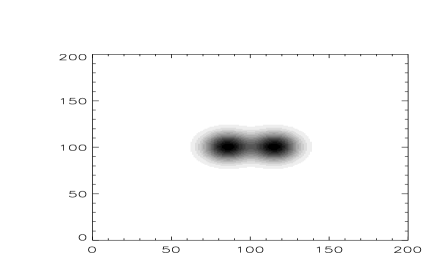
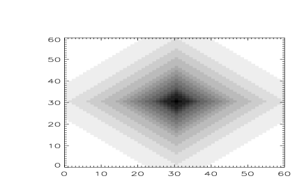
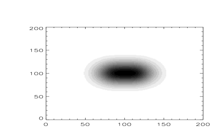
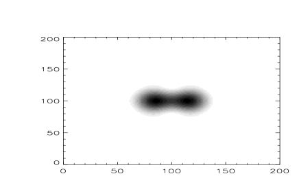
Figure 1: Example of deconvolution by shapelet decomposition: (a) Image before smearing, (b) Convolving kernel (PSF), (c) Smeared image, (d) Recovered image from the shapelet matrix inversion.

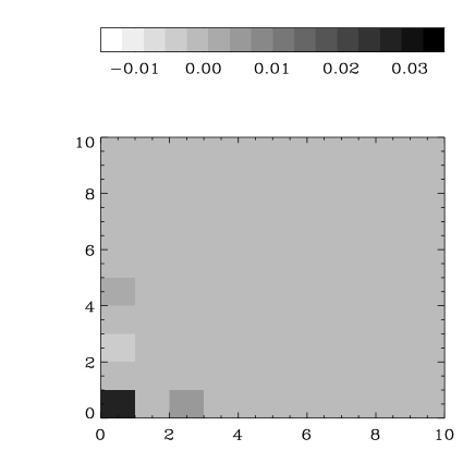
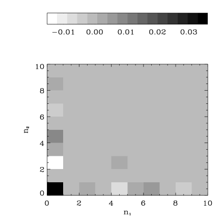
Figure 2: Coefficient matrices at different stages of the deconvolution shown in Figure 1: (a) original image, (b) convolved image, (c) deconvolved image.

As Kuijken (2000) suggested, another approach consists in fitting the observed galaxy coefficients ${\mathbf{h}}=\{h_{\mathbf{n}}\}$ for the deconvolved coefficients ${\mathbf{f}}=\{f_{\mathbf{n}}\}$. This can be done by minimizing

$$\chi^{2}=({\mathbf{h}}-{\mathbf{P}}{\mathbf{f}})^{T}{\mathbf{V}}^{-1}({\mathbf{h}}-{\mathbf{P}}{\mathbf{f}}),$$ (14)

with respect to the model parameters ${\mathbf{f}}$ given the data vector ${\mathbf{h}}$. Here, $V_{\mathbf{n}m}={\rm cov}(h_{\mathbf{n}},h_{\mathbf{m}})$ is the covariance of the observed coefficients $h_{\mathbf{n}}$ resulting from noise in the observed image. As discussed in Paper I, this can easily be evaluated from the properties of the pixel noise. For instance, it is proportional to the identity matrix in the case of white noise. Since this model is linear in the model parameters ${\mathbf{f}}$, the best fit has the simple analytic solution (see eg. Lupton 1993)

$${\mathbf{f}}=({\mathbf{P}}^{T}{\mathbf{V}}^{-1}{\mathbf{P}})^{-1}{\mathbf{P}}^{T}{\mathbf{V}}^{-1}{\mathbf{h}},$$ (15)

with a covariance error matrix $W_{\mathbf{n}m}={\rm cov}(f_{\mathbf{n}},f_{\mathbf{m}})$ given by ${\mathbf{W}}=({\mathbf{P}}^{T}{\mathbf{V}}^{-1}{\mathbf{P}})^{-1}$. These analytic solutions make the best fit parameters and errors efficient to evaluate in practice.

The latter scheme is potentially more robust numerically since it does not require the direct inversion of the PSF matrix. On the other hand, it is more complicated and requires knowledge of the noise properties of the observed image. In particular, the $\chi^{2}$ procedure is, strictly speaking, only valid in the case of gaussian noise, a condition never rigorously met in optical CCD images. We have tried both deconvolution schemes on various object and PSF shapes and have found that they both perform equally well (as long as the PSF matrix is restricted to low-order as discussed above). For the remainder of this paper, we will use the direct inversion scheme, i.e. Equation (13).

Figure 1 gives an illustration of the procedure. A galaxy (panel 1) is smeared by a complicated PSF (panel 2). The resulting object is shown in panel 3. The deconvolved galaxy image obtained using our direct inversion scheme (using $n_{\rm max}=9$, $\beta=15$ and $\alpha=\gamma=20$ pixels) is shown on panel 4. It is very close to panel 1, showing that our method is successful in recovering the original image. A deconvolution using the $\chi^{2}$ method yields very similar results. Figure  2 shows the shapelet coefficient matrix at different stages of the procedure. Notice the projection of high-order coefficients for the galaxy (panel 1) into lower-order coefficients after convolution (panel 2). The recovered coefficients (panel 3) are very close to the original coefficients (panel 1).

4 Measure of the Shear

Now that we have a method to correct for the PSF, we turn to the problem of measuring the shear from an ensemble of galaxies. We start by presenting the formalism used to describe the action of shear with shapelets. We then construct shear estimators for each shapelet coefficient and combine them to derive a minimum variance estimator.

4.1 Shear Matrix

Let us consider a galaxy with an unlensed intensity $f({\mathbf{x}})$. In our formalism (see Paper I), the lensed intensity after a weak shear $\gamma_{i}$ is written as

$$f^{\prime}\simeq(1+\gamma_{i}\hat{S}_{i})f,$$ (16)

to first order in the shear, where $\hat{S}_{i}$ is the shear operator. If we decompose these intensities into our basis functions $B_{{\mathbf{n}}}({\mathbf{x}},\beta)$ (Eq. [3]), this can be expressed as a relation between the lensed and the unlensed coefficients:

$$f^{\prime}_{{\mathbf{n}}}=(\delta_{\mathbf{n}m}+\gamma_{i}S_{i{\mathbf{n}m}})f_{{\mathbf{m}}},$$ (17)

where $S_{i{\mathbf{m}n}}\equiv\int d^{2}xB_{{\mathbf{n}}}({\mathbf{x}})\hat{S}_{i}B_{{\mathbf{m}}}({\mathbf{x}})$ is the shear matrix. As presented in Paper I, our basis functions are also the eigenfunctions for the Quantum Harmonic Oscillator (QHO), thus allowing us to use the powerful formalism developed for this problem. In particular, the shear operators can be written as

$$\hat{S}_{1} = \frac{1}{2}\left(\hat{a}_{1}^{\dagger 2}-\hat{a}_{2}^{\dagger 2}-\hat{a}_{1}^{2}+\hat{a}_{2}^{2}\right)$$

$$\hat{S}_{2} = \hat{a}_{1}^{\dagger}\hat{a}_{2}^{\dagger}-\hat{a}_{1}\hat{a}_{2},$$ (18)

where $\hat{a}^{\dagger}_{i}$ and $\hat{a}_{i}$ are the raising and lowering operators, for each dimension $i=1,2$. They operate as

$$\hat{a}_{1}B_{n_{1},n_{2}}=\sqrt{n_{1}}B_{n_{1}-1,n_{2}},~{}~{}~{}\hat{a}_{1}^{\dagger}B_{n_{1},n_{2}}=\sqrt{n_{1}+1}B_{n_{1}+1,n_{2}},$$ (19)

and similarly for $\hat{a}_{2}$ and $\hat{a}^{\dagger}_{2}$. The shear matrices are thus simple to evaluate in this way, and are very sparse since they involve the mixing of only a few modes.

An illustration of the action of the shear matrix on the first few shapelet states can be found in Paper I. A more realistic example is shown on Figure 3. Here, we have used the shear matrix to shear a galaxy (panel 1) found in the Hubble Deep Field (Williams et al. 1996) by 20%. The resulting sheared image (panel 2) is virtually indistinguishable from the same image sheared directly in real space (panel 3). The action of shear on the shapelet coefficients is illustrated in figure 4. The average shapelet coefficients for a population of galaxies in one of our simulations (see §6) is shown in the upper panel. The difference between the coefficients before and after shears of 20% in the $\gamma_{1}$ and $\gamma_{2}$ directions are shown in the middle and lower panels, respectively. Note the change in even-even coefficient components associated with a shear in the $\gamma_{1}$ direction, and the change in odd-odd coefficients for a shear in the $\gamma_{2}$ direction (see below for a discussion of this effect).

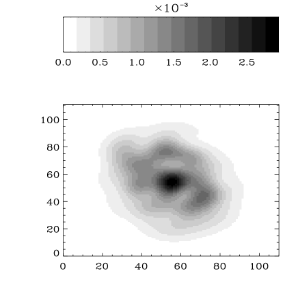
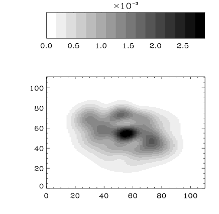
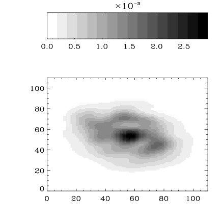
Figure 3: Example of the action of the shear matrix on a galaxy found in the Hubble Deep Field. The original image (panel 1) is sheared by 20% by the shear matrix (panel 2). The resulting image is almost indistinguishable from that of the same galaxy sheared directly in real space (panel 3).

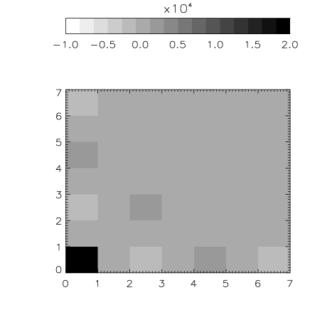
Figure 4: Action of shear on the average shapelet coefficients for a galaxy population in our simulation: (a) Initial simulation, (b) difference between initial and sheared simulation coefficients $(\gamma_{1}=0.2)$, (c) same as (b) for $\gamma_{2}=0.2$.

4.2 Shear Estimator

Our goal is to find an estimator $\widetilde{\gamma}_{i}$ for the shear $\gamma_{i}$. We require that this estimator be unbiased, i.e. that $\langle\widetilde{\gamma}_{i}\rangle=\gamma_{i}$, when averaged over a population of galaxies which are randomly oriented before lensing. To limit the impact of noise on our estimator, we also require it to be linear in the sheared coefficients $f^{\prime}_{\mathbf{n}}$.

To construct such an estimator, we first notice that the average shapelet coefficients $\langle f_{\mathbf{n}}\rangle$, before lensing, must be rotationally invariant. This must be so since the ensemble of randomly-oriented galaxies does not have a preferred direction. Using the polar shapelets discussed in §5 of Paper I, it is easy to show that this will be satisfied only if $\langle f_{\mathbf{n}}\rangle$ vanishes when $n_{1}$ and/or $n_{2}$ is odd. This can be verified by inspecting the top panel of Figure 4, which shows that the only non-zero unlensed coefficients are the even-even ones, in a simulated galaxy ensemble (see §6).

The coefficients $f^{\prime}_{\mathbf{n}}$ after lensing will no longer have this symmetry, since the shear introduces a preferred direction. In our formalism, this results from the mixing induced by the shear operator (see Eq. [17]). From Equation (4.1), it is easy to see that a $\gamma_{1}$-shear mixes even-even states along the vertical and horizontal axes in the $n_{1}-n_{2}$ shapelet coefficient plane. On the other hand, a $\gamma_{2}$-shear mixes states diagonally on this plane. As a result, $\gamma_{1}$ only affects states with $n_{1}$ and $n_{2}$ even, while $\gamma_{2}$ only those with $n_{1}$ and $n_{2}$ odd. (States with $n_{1}$ even and $n_{2}$ odd, or vice-versa, are left unchanged by shear). This convenient fact means that the two shear components are decoupled in shapelet space (see figure 4). We can therefore construct independent estimators for each component. It is easy to show, that the only estimators satisfying the above conditions are

$$\widetilde{\gamma}_{1{\mathbf{n}}} = \frac{f^{\prime}_{\mathbf{n}}-\langle f_{\mathbf{n}}\rangle}{S_{1{\mathbf{n}m}}\langle f_{\mathbf{m}}\rangle},~{}~{}n_{1},n_{2}~{}{\rm even}$$

$$\widetilde{\gamma}_{2{\mathbf{n}}} = \frac{f^{\prime}_{\mathbf{n}}-\langle f_{\mathbf{n}}\rangle}{S_{2{\mathbf{n}m}}\langle f_{\mathbf{m}}\rangle},~{}~{}n_{1},n_{2}~{}{\rm odd},$$ (20)

where only even-even (odd-odd) coefficients are used for $\widetilde{\gamma}_{1{\mathbf{n}}}$ ($\widetilde{\gamma}_{2{\mathbf{n}}}$). As before, the brackets denote an average over the galaxy ensemble and can be estimated using a large region where the mean shear is effectively 0. This provides us with a shear estimator $\widetilde{\gamma}_{i{\mathbf{n}}}$ for every (appropriate) shapelet coefficient of each galaxy.

We now seek to combine these estimators in a manner which maximises the shear signal. For this purpose, we can construct a combined shear estimator of the form

$$\widetilde{\gamma}_{i}=\frac{\sum_{\mathbf{n}}w_{i{\mathbf{n}}}\widetilde{\gamma}_{i{\mathbf{n}}}}{\sum_{\mathbf{n}}w_{i{\mathbf{n}}}},$$ (21)

where the weights $w_{1{\mathbf{n}}}$ ($w_{2{\mathbf{n}}}$) are set to zero when ${\mathbf{n}}$ is not even-even (odd-odd). By construction, $\widetilde{\gamma}_{i}$ is still linear and, thanks to the denominator, guaranteed to be unbiased. The weights then need to be chosen to minimise the uncertainty in $\widetilde{\gamma}_{i}$. To find the optimal weights, we consider the covariance matrix between the individual estimators

$$V_{i{\mathbf{n}m}}\equiv{\rm cov}(\widetilde{\gamma}_{i{\mathbf{n}}},\widetilde{\gamma}_{i{\mathbf{m}}}),$$ (22)

which can be computed by averaging over the (unsheared) galaxy ensemble. It is easy to show that the variance ${\rm var}(\widetilde{\gamma}_{i})$ of the combined estimator is minimized when

$$w_{i{\mathbf{n}}}=\sum_{\mathbf{m}}V^{-1}_{i{\mathbf{n}m}}.$$ (23)

With this optimal choice for weights $w_{i{\mathbf{n}}}$, the estimator variance reduces to

$${\rm var}(\widetilde{\gamma}_{i})=\left(\sum_{\mathbf{n}m}V^{-1}_{i{\mathbf{n}m}}\right)^{-1}.$$ (24)

We have thus derived an optimal shear estimator (Eq. 21) for each galaxy. It can then be averaged over all galaxies in a region to provide a local estimate of the shear. The error in the resulting shear measurement can then be computed using Equation (24), or directly from the variance of the actually measured shear estimators. We now discuss how to implement the shear estimation in practice.

5 Implementation

The above formalism is fairly straightforward, and is easily implemented. Here we describe some important practical details which are required for measuring shear from real data.

The objects in an image are first detected and catalogued using the publicly available software SExtractor (Bertin & Arnouts 1996). Each object is then cut out from the image, choosing a square centred upon the SExtractor centroid, extending by 5 times the SExtractor semi-major axis found for the object. This ensures that the box size is much larger than the object, as is necessary for the orthogonality of the basis functions. The median background around each of these objects is then subtracted.

Stars are selected, either from a magnitude-radius plot or from the SExtractor neural network classifier. The stars are decomposed into shapelet coefficients, choosing $\beta$ to be 0.7 times the semi-major axis found by SExtractor (this choice is convenient as it leads to a compact PSF representation in shapelet space). We iterate to find the best centroid for decomposition by decomposing a first time, finding a new centroid using Equation (27) in Paper I, then decomposing a second time about the new centroid. For this paper, we set the maximum order of the stellar decomposition to $n_{\rm max}=6$. Each stellar shapelet component is divided by the stellar flux calculated from Equation (26) in Paper I, thus yielding normalised stellar coefficients.

We can then interpolate each stellar normalised coefficient across the field using a 2-dimensional polynomial. This affords us with a model of the PSF at each point on the image, which we can then use to deconvolve the galaxies. In the simulation described below (§6), the PSF is constant across the field. In this paper, we thus simply average the coefficients from all stars, and use this average coefficient set for desmearing at all positions in the field.

We now decompose each galaxy according to Equation (3), using $n_{\rm max}=6$ as before. We choose the shapelet scale for the galaxies to be fixed to the median SExtractor FWHM for the set of galaxies in question (see discussion of binning below). In the case of galaxies where this scale is close to the decomposition scale for stars ($\beta$), we set the decomposition scale to $1.5\beta$. As for the stars, we iterate to obtain the best centroid about which to decompose.

We then deconvolve each galaxy with the PSF model at that position, using Equation (13). To make the matrix inversion stable (see §3), we only keep a finite number of elements of the PSF matrix, here $n_{\rm max}=6$. (We could alternatively apply the $\chi^{2}$ modelling of Eq. [15]). The best results are obtained by choosing the deconvolved shapelet scale $\alpha$ to be equal to $\gamma$. Indeed, a choice of $\alpha$ comparable to $\gamma$ uses all the available information, and does not prohibit us from recovering small objects.

The next step is to bin the galaxies by magnitude and radius. This is to reduce the dispersion in the shapelet coefficients, and therefore the overall uncertainty of the combined shear estimators. The choice of bin size depends on the size of the data set, as each bin should contain enough objects to afford reasonable signal-to-noise in the bin. For each bin we obtain shear estimators $\widetilde{\gamma}_{i{\mathbf{n}}}$ from all (appropriate) coefficients ${\mathbf{n}}$, using Equation (4.2). We then calculate the weight $w_{i{\mathbf{n}}}$ for each shear estimator according to Equation (23), and compute the combined estimator for this galaxy (Eq. [21]).

Next we perform an (unweighted) average of the shear estimators for all galaxies within a given magnitude-radius bin. We can finally perform a weighted average of the shear estimators from all bins, using the variance within each bin as the inverse weight; we can even weight with magnitude in order to optimise the weak-lensing signal from a given redshift interval.

6 Simulations

We now describe our initial tests of this new method using simulations. Our goal is to verify that our method can recover shear which we impose upon simulated images with realistic observational properties. A further paper (Bacon et al 2001b) will describe a range of ground- and space-based applications, and compare results obtained with KSB and shapelets for simulated and real data. Here we restrict ourselves to ground-based applications, while recognising that the preservation of more than second moments with shapelets will have greatest initial impact on shear measurements from space.

The simulations are based on those described in Bacon et al. (2001a). Full details are contained in that paper; here we briefly summarise the relevant features of the simulations. We create realistic simulations of fields of galaxies observed by a typical ground-based 4m telescope (the William Herschel Telescope), with appropriate magnitudes, counts, diameters and ellipticities for stars and galaxies. We include an appropriate range of seeing, input shear, and tracking errors, and set the simulations in the context of the appropriate pixel scale.

We obtain the required galaxy statistics via the the resolved (0.1 arcsec seeing) image statistics of the Groth Strip (Groth et al. 1994), a deep ($I\simeq 26$) survey observed by the Hubble Space Telescope (cf Bacon et al 2001a). Since the HST PSF is much smaller than that typical for WHT (0.7”), the Groth Strip provides effectively unsmeared ellipticities and diameters. The Groth Strip contains approx. 10,000 galaxies in a 108 arcmin² area. We utilise Ebbels’ (1998) SExtractor catalogue obtained from the strip, which contains magnitude, diameter, and ellipticity for each object.

We fit a model to the multi-dimensional probability distribution of galaxy properties (eg morphology, ellipticity, diameter, magnitude) in this catalogue. With the resulting model, we can draw a statistically similar catalogue of galaxies with a realistic distribution of these properties, via Monte Carlo selection. We spatially distribute the objects randomly over a CCD frame, and add stars of appropriate magnitude distribution modelled from WHT data.

It is now a simple matter to shear the galaxies in our catalogue. We first calculate the change in each object’s ellipticity $e_{i}$ which lensing will induce. To first order in the shear, the ellipticity transforms as (see Rhodes et al 2000)

$$e^{\prime}_{i}=e_{i}+2(\delta_{ij}+e_{i}e_{j})\gamma_{j}.$$ (25)

Similarly, the magnitude of the sheared object is related to that of the initial object by

$$m^{\prime}=m+2.5\log(1-\gamma^{2})$$ (26)

Finally, we compute the sheared semi-major axis size. In order to do this, we define $R,A$ and $J$ matrices by

$$R=\left(\begin{array}[]{cc}\cos\phi&\sin\phi\\ -\sin\phi&\cos\phi\\ \end{array}\right)$$ (27)

$$A=\left(\begin{array}[]{cc}a^{2}&0\\ 0&b^{2}\\ \end{array}\right)$$ (28)

$$J=R^{T}AR$$ (29)

where $\phi$ is the position angle of the object in question, $a$ is its semi-major axis, and $b$ its semi-minor axis. Then, if we define a shear matrix $\Phi$ as

$$\Phi=\left(\begin{array}[]{cc}\gamma_{1}&\gamma_{2}\\ \gamma_{2}&-\gamma_{1}\\ \end{array}\right)$$ (30)

we can find the new semi-major axis $a^{\prime}$ using

$$J^{\prime}_{k,l}=J_{k,l}+J_{k,i}\Phi_{l,i}+J_{l,i}\Phi_{k,i}\\$$ (31)

$$a^{\prime 2}=0.5\left(J^{\prime}_{0,0}+J^{\prime}_{1,1}+\sqrt{(J^{\prime}_{0,0}-J^{\prime}_{1,1})^{2}+4{J^{\prime}_{0,1}}^{2}}\right).$$ (32)

These relations provide us with the sheared object catalogue.

For the purposes of this paper, we ran a set of simulations with shears in both $\gamma_{1}$ and $\gamma_{2}$ directions, ranging from zero to 5%. This affords a check of the shapelet method in the weak shear regime. We set a shear which is uniform over a given field. This is adequate for our initial tests, in which we are interested in recovering a mean shear across a whole field.

We model tracking errors by giving an anisotropic PSF to the fields. Stellar ellipticities are chosen as uniform across a given field, with the variance of the ellipticity from field to field equal to $\sigma_{e}$=0.05.

We produce simulated images from the catalogues with the IRAF artdata package. This draws stars and galaxies from the catalogues with specified magnitude, diameter, ellipticity, morphology (de Vaucouleurs or exponential) and position. Telescope-specific details are included: telescope throughput, anisotropic PSF (with Moffatt profile, and seeing chosen to be 0.6”), pixellisation (0.24” per pixel), Poisson and read noise, sky background and gain are all realistically modelled. Examples of the resulting images can be found in Bacon et al (2001a).

After image realisation, we apply our shear measurement algorithm to the simulated images. We train the estimators (i.e. obtain the necessary $\langle f_{\mathbf{n}}\rangle$ for Eq. [4.2]) with an unsheared set of galaxies with the magnitude-radius distribution and intrinsic properties appropriate for our selected cell. For our testing purposes, we examine the shear in one narrow magnitude-radius bin only, centred on $m=22.5$ and $a=2.0$ pixels.

We compare the input shear for our simulated fields with the shear estimates obtained by the shapelets method. The results are shown in figure 5 for the 0-5% shear simulations described above. Notice that the output shear is linearly related to input shear, with a slope consistent with 1. With linear regression we indeed find $\gamma^{{\rm out}}_{1,i}=0.97\gamma^{{\rm in}}_{1,i}$ and $\gamma^{{\rm out}}_{2,i}=1.00\gamma^{{\rm in}}_{2,i}$, with standard errors on the slope of 0.04 in each case.

We conducted a further set of simulations to examine the effect of seeing (PSF size) on our recovery. A set of simulations with identical shear $(\gamma_{1},\gamma_{2})=(0.00,0.05)$ were produced, with seeing values ranging from 0.2” to 0.8”. The recovery and noise are demonstrated in Figure 6. Our method clearly remains unbiased at all seeing values considered. Since we examine the shear in a single, small magnitude bin, the number density does not increase to improve the signal with decreased PSF, as is the case when all magnitudes are considered (see Bacon et al 2001). Nevertheless, a small decrease in noise is seen at small seeing values, showing that more information is recovered in this case.

Figure 5: Input shear vs recovered shear for a set of 11 simulations.

Figure 6: Results for set of simulations showing shear recovery with varying seeing. Note the excellent recovery at all seeing values, with slight increase in noise with increasing PSF.

These initial simulations demonstrate the effectiveness and utility of this shear measurement method. We have made additional tests to check the reliability of the method upon varying galaxy type, size and magnitude; the shear is recovered accurately in each case. Detailed discussion of these properties of the method on real and simulated data will be carried out in a further paper (Bacon et al 2001b).

7 Conclusions

In this paper, we have presented a new method for precision measurements of weak lensing. After summarising the necessary formalism from Paper I, we described the means of convolving and deconvolving objects using shapelets. In shapelet space, this is a simple matrix operation, which can be used to correct for the PSF. We then presented shear estimators for shapelets. These are obtained from another simple matrix formalism, and are constructed to be unbiased and linear. Each shapelet coefficient (even-even and odd-odd) provides a shear estimator, thus using all the available shape information for each object. We combined these individual estimators to construct a minimum variance estimator for the shear, ensuring that the shear signal is maximised.

The reliability of our shapelet method was then tested using simulations of realistic ground-based images. We find the method to be accurate and stable against variation of galaxy type, size of object, noise level, and PSF characteristics. In a future paper (Bacon et al 2001b), we will present detailed tests of our method based on extensive ground- and space- based image simulations. In particular, we will compare in detail the performance of our method against that of the commonly used KSB method.

Compared to other methods, the advantages of our method lie in several areas. Firstly, the remarkable properties of the shapelet basis functions turn operations such as convolution and shear into simple and analytic matrix operations. In particular, the shear operator can be expressed as a simple combination of raising and lowering operators, borrowed from the formalism of the QHO. Secondly, it is linear in the galaxy intensity, thus avoiding biases introduced by imperfect knowledge of the noise property of the image. Thirdly, the shapelet formalism is capable of using all the available shape information, and of optimally estimating shear from it. For instance, the KSB method only considers gaussian-weighted quadrupole moments, which are exactly equal to our second-order shapelet moments. Our method thus, in a sense, generalises the KSB approach to include all available high-order moments. Finally, the method is analytic and well-defined mathematically, and is thus more reliable and stable than KSB which is known to suffer from ill-defined quantities (see Kuijken 1999; Kaiser 2000).

Thanks to these advantages and to its overall completeness and clarity, our method is well-placed for the analysis of current and future weak shear surveys. In particular, it will allow us to fully exploit the remarkable resolution of future space-based weak lensing surveys with HST and the planned SNAP mission (Perlmutter et al. 2001). It thus promises to provide the sophistication necessary to enter the next stage of high-precision shear analysis.

References

- [1] Bacon, D., Refregier, A., Ellis, R., 2000, MNRAS, 318, 625.
- [2] Bacon, D., Refregier, A., Clowe, D., Ellis, R., 2001a, to appear in MNRAS, preprint astro-ph/0007023.
- [3] Bacon, D., Refregier, A. et al., 2001, in preparation
- [4] Bartelmann, M., & Schneider, P. 2000, preprint astro-ph/0007023
- [5] Bernardeau, F., van Waerbeke, L., & Mellier, Y., 1997, A&A, 322, 1.
- [6] Bertin E., & Arnouts S., 1996, A&AS, 117, 393
- [7] Bonnet H., Mellier Y., 1995, A&A, 303, 331
- [8] Chang, T.-Z., & Refregier, A. 2001, in preparation
- [9] Ebbels, T., 1998, Ph.D. thesis, University of Cambridge
- [10] Erben, T., van Waerbeke, L., Bertin, E., Mellier, Y., Schnedier, P., 2001, A&A, 366, 717.
- [11] Groth et al., 1994, BAAS, 185, 5309
- [12] Kaiser, N., Squires, G., Broadhurst, T., 1995, ApJ, 449, 460.
- [13] Kaiser, N., 2000, ApJ, 537, 555.
- [14] Kaiser, N., Tonry, J. N., Luppino, G. A., 2000, PASP, 112, 768.
- [15] Kaiser, N., Wilson, G., Luppino, G. A., 2000, preprint astro-ph/0003338
- [16] Kuijken, K., 1999, A&A, 352, 355.
- [17] Lupton, R. 1993, Statistics in Theory and Practice, (Princeton U. Press: Princeton).
- [18] Mellier, Y. 1999, ARA&A, 37, 127
- [19] Maoli, R. et al, 2001, A&A, 368, 766.
- [20] Refregier, A. 2001, (Paper I) submitted to MNRAS, preprint available on astro-ph
- [21] Rhodes, J., Refregier, A., & Groth, E. 2000, ApJ, 536, 79
- [22] Rhodes, J., Refregier, A., & Groth, E., 2001, to appear in ApJL, preprint astro-ph/0101213
- [23] Taylor, A. et al, 2001, in preparation
- [24] Tyson, J. A., Wittman, D., & Angel, J. R. P., 2000, in Procs. of Dark Matter 2000 conference, Santa Monica Feb 2000, preprint astro-ph/0005381.
- [25] van Waerbeke, L. et al, 2000, A&A, 358, 30.
- [26] van Waerbeke, L. et al, 2001, submitted to A&A, preprint astroph/0101511.
- [27] Williams et al. 1996, AJ, 112, 1335
- [28] Wittman, D., Tyson, J. A., Kirkman, D., Dell’Antonio, I., Bernstein, G., 2000, Nature, 405, 143.