Shapelets: I. A Method for Image Analysis

Abstract

We present a new method for the analysis of images, a fundamental task in observational astronomy. It is based on the linear decomposition of each object in the image into a series of localised basis functions of different shapes, which we call ‘Shapelets’. A particularly useful set of complete and orthonormal shapelets is that consisting of weighted Hermite polynomials, which correspond to perturbations around a circular gaussian. They are also the eigenstates of the 2-dimensional Quantum Harmonic Oscillator, and thus allow us to use the powerful formalism developed for this problem. Among their remarkable properties, they are invariant under Fourier transforms (up to a rescaling), leading to an analytic form for convolutions. The generator of linear transformations such as translations, rotations, shears and dilatations can be written as simple combinations of raising and lowering operators. We derive analytic expressions for practical quantities, such as the centroid (astrometry), flux (photometry) and radius of the object, in terms of its shapelet coefficients. We also construct polar basis functions which are eigenstates of the angular momentum operator, and thus have simple properties under rotations. As an example, we apply the method to Hubble Space Telescope images, and show that the small number of shapelet coefficients required to represent galaxy images lead to compression factors of about 40 to 90. We discuss applications of shapelets for the archival of large photometric surveys, for weak and strong gravitational lensing and for image deprojection.

1 Introduction

Image analysis is a fundamental task in observational astronomy. For instance, new techniques, such as weak gravitational lensing (see reviews by Mellier 1999; Bartelmann & Schneider 2000), microlensing (Mao 1999) and the search for supernovae (Riess 2000; Perlmutter et al. 1998), have great scientific promise, but require high precision image processing and analysis. As a result, a number of sophisticated data analysis packages (eg. FOCAS in IRAF, Jarvis & Tyson 1986; SExtractor, Bertin & Arnouts 1996, etc) and techniques (eg. wavelet analysis, see review by Stark, Murtagh & Bijaoui 1998; image subtraction, Alard & Lupton 1998; shear measurement, Kaiser, Squires & Broadhurst 1995, Kaiser 2000, and Kuijken 2000) have been developed.

In this paper, we present a new method for image analysis. It is based on the linear decomposition of each object into a series of localised basis functions with different shapes, which we call ‘Shapelets’. As a basis set we choose weighted hermite polynomials. They correspond to perturbations about a circular gaussian, and, in their asymptotic form, to the Edgeworth expansion in several dimensions. They are also the eigenstates of the 2-dimensional Quantum Harmonic Oscillator (QHO), and thus allow us to use the powerful formalism developed for this problem. They have remarkable properties. In particular, they are (up to a rescaling) invariant under Fourier transforms and thus yield a simple analytical form for convolutions. We derive a number of practical tools which can use used to compute the characteristics of the object (centroid, flux, radius, etc) from its shapelet coefficients. Our method differs from the wavelet transform which decomposes the image into a sum of basis functions of different scales but with a set shape. In our method, the image is decomposed into a collection of compact disjoint objects of arbitrary shapes and is thus particularly adapted to astronomical images.

As an example, we show how images of galaxies observed with the Hubble Space Telescope (HST) can be represented and strongly compressed using shapelets. We also discuss several applications of shapelets, such as archival of large photometric catalogues, gravitational lensing and image de-projection. A precise method to measure the shear induced by weak lensing on galaxy images is presented in an adjoining paper (Refregier & Bacon 2001, Paper II). The application of Shapelets to interferometric images will be presented in Chang & Refregier (2001). The analytical results derived in this paper may also be useful for any application using the Edgeworth expansion, such as, for instance, the study of the growth of cosmological perturbations (Juskiewicz et al. 1995 and reference therein).

This paper is organised as follows. In §2, we describe the main properties of 1-dimensional shapelets and discuss their connection to the QHO. In §3, we show how 2-dimensional shapelets can be formed and derive a number of practical analytical results. In §4, we discuss how the shapelet states behave under convolutions. In §5, we derive polar shapelets from the cartesian basis functions and describe some of their properties. In §6, we discuss several direct applications of shapelets. Our conclusions are presented in §7.

2 One-Dimensional Shapelets

2.1 Definitions

We first consider the description of a localised object in 1-dimension. For this purpose, we first define the dimensionless basis functions

$$\phi_{n}(x)\equiv\left[2^{n}\pi^{\frac{1}{2}}n!\right]^{-\frac{1}{2}}H_{n}(x)e^{-\frac{x^{2}}{2}}$$ (1)

where $n$ is a non-negative integer and $H_{n}(x)$ is a hermite polynomial of order $n$. These functions are orthonormal in the sense that

$$\int_{-\infty}^{\infty}dx~{}\phi_{n}(x)\phi_{m}(x)=\delta_{nm},$$ (2)

where $\delta_{mn}$ is the Kronecker delta symbol. The first few functions are plotted on figure 1. These functions, which we call ‘Shapelets’, can be thought of as shape perturbations around the gaussian $\phi_{0}(x)$,

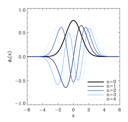
Figure 1: First few 1-dimensional basis functions $\phi_{n}(x)$.

To describe an object in practice, we use the dimensional basis functions

$$B_{n}(x;\beta)\equiv\beta^{-\frac{1}{2}}\phi_{n}(\beta^{-1}x),$$ (3)

where $\beta$ is a characteristic scale, which is typically chosen to be close to the size of the object. These functions are also orthonormal, i.e.

$$\int_{-\infty}^{\infty}dx~{}B_{n}(x;\beta)B_{m}(x;\beta)=\delta_{nm}.$$ (4)

This infinite set of functions forms a complete basis for smooth and integrable functions. Thus, a (sufficiently well behaved) object profile $f(x)$ can be expanded as

$$f(x)=\sum_{n=0}^{\infty}f_{n}B_{n}(x;\beta).$$ (5)

From the orthonormality condition (Eq. [4]), the shapelet coefficients are given by

$$f_{n}=\int_{-\infty}^{\infty}dx~{}f(x)B_{n}(x;\beta).$$ (6)

In practice, the series of Equation (5) will converge quickly if the object $f(x)$ is sufficiently localised, and if $\beta$ and the origin $x=0$ are not too different from the size and location of the object. This series representation is referred to as the Gram-Charlier series, or, in its asymptotic form, as the Edgeworth expansion (see eg. Juiszkiewicz 1995 and reference therein).

2.2 Fourier Transform

These basis functions have a number of useful properties. Let us first consider their Fourier transform, which, for an arbitrary function $f(x)$, is defined as

$$\tilde{f}(k) = (2\pi)^{-\frac{1}{2}}\int_{-\infty}^{\infty}dxf(x)e^{ikx},$$

$$f(x) = (2\pi)^{-\frac{1}{2}}\int_{-\infty}^{\infty}dk\tilde{f}(k)e^{-ikx}.$$ (7)

With these conventions, the Fourier transform of the dimensionless basis function $\phi_{n}(\xi)$ is

$$\widetilde{\phi}_{n}(\kappa)=i^{n}\phi_{n}(\kappa),$$ (8)

Thus, up to a phase factor, the dimensionless basis functions are invariant under Fourier transforms. This very useful property can be understood in physical terms from the analogy with the quantum harmonic oscillator (see §2.3).

The Fourier transform of the dimensional basis function $B_{n}(x;\beta)$ is given by

$$\widetilde{B}_{n}(k;\beta)=i^{n}B_{n}(k;\beta^{-1}).$$ (9)

Thus, the Fourier transform acts on the basis functions with an unsurprising change of scale $\beta\rightarrow\beta^{-1}$.

2.3 Analogy with the Quantum Harmonic Oscillator

As we now discuss, the above basis functions are the eigenstates of the Quantum Harmonic Oscillator (QHO), which allows us to exploit the readily available formalism developed for this problem. Let us consider a QHO with mass $m$ and natural frequency $\omega$. If distances are measured in units of $\sqrt{\frac{\hbar}{m\omega}}$ and energies in units of $\hbar\omega$, the Hamiltonian for this system is

$$\hat{H}=\frac{1}{2}\left[\hat{x}^{2}+\hat{p}^{2}\right]$$ (10)

where $\hat{x}$ and $\hat{p}$ are the position and momentum operators respectively. In the $x$-representation, they are given by

$$\hat{x}=x,~{}~{}~{}\hat{p}=\frac{1}{i}\frac{\partial}{\partial x},$$ (11)

and commute as $[\hat{x},\hat{p}]=i$. As is well known, the basis functions $\phi_{n}(x)$ are the eigenfunctions of the Hamiltonian, with

$$\hat{H}\phi_{n}=\left(n+\frac{1}{2}\right)\phi_{n}.$$ (12)

Clearly, $\hat{H}$ is symmetric under a permutation of $\hat{x}$ and $\hat{p}$ (see Eq. [10]), thus explaining the invariance of $\phi_{n}$ under Fourier transforms (Eq. [8]).

Of particular practical interest are the lowering and raising operators, which are defined as

$$\hat{a}\equiv\frac{1}{\sqrt{2}}\left(\hat{x}+i\hat{p}\right),~{}~{}~{}\hat{a}^{\dagger}\equiv\frac{1}{\sqrt{2}}\left(\hat{x}-i\hat{p}\right),$$ (13)

where ^† is the Hermitian conjugate. They commute as $[\hat{a},\hat{a}^{\dagger}]=1$, and act on the basis functions as

$$\hat{a}\phi_{n}=\sqrt{n}\phi_{n-1},~{}~{}~{}\hat{a}^{\dagger}\phi_{n}=\sqrt{n+1}\phi_{n+1}.$$ (14)

The Hamiltonian can then be rewritten as $\hat{H}=\hat{N}+\frac{1}{2}$, where the number operator $\hat{N}\equiv\hat{a}^{\dagger}\hat{a}$ has the property that

$$\hat{N}\phi_{n}=n\phi_{n}.$$ (15)

When convenient, we will use the bra-ket notation of quantum mechanics. For instance, the $n^{\rm th}$ state is written as $|n\rangle$ and has an $x$-representation given by $\langle x|n\rangle=\phi_{n}(x)$.

The dimensional basis functions are the eigenfunctions of the Hamiltonian

$$\hat{H}_{\beta}=\frac{1}{2}\left[\beta^{-2}\hat{x}^{2}+\beta^{2}\hat{p}^{2}\right].$$ (16)

The eigenstates are labeled as $|n;\beta\rangle$ and obey $\hat{H}_{\beta}|n;\beta\rangle=\left(n+\frac{1}{2}\right)|n;\beta\rangle$. The dimensional basis functions are then given by $B_{n}(x;\beta)=\langle x|n;\beta\rangle$.

2.4 Further Properties

The Hermite basis functions have a number of further convenient properties which we will need later and summarise here.

We first notice, by inspecting Figure 1, that the basis functions $B_{n}(x,\beta)$ acquire both a larger extent and smaller scale oscillations when the order $n$ is increased, keeping $\beta$ constant. This can be described more precisely by considering the characteristic radius $\theta_{\rm max}(\beta,n)$ of a basis function, defined by $\theta_{\rm max}^{2}(\beta,n)\equiv\langle n;\beta|\hat{x}^{2}|n;\beta\rangle$. As is well known from Quantum Mechanics and can easily derived using Equation (13), this rms radius is given by $\theta_{\rm max}(\beta,n)=\beta\left(n+\frac{1}{2}\right)^{\frac{1}{2}}$. Similarly, the characteristic size $\theta_{\rm min}(\beta,n)$ of the small scale (oscillatory) features in a basis function of order $n$ is defined as the rms inverse radius in Fourier space, i.e. by $\theta_{\rm min}^{-2}(\beta,n)\equiv\langle n;\beta|\hat{p}^{2}|n;\beta\rangle$. As can again be verified using raising and lower operators, the radius is given by $\theta_{\rm min}(\beta,n)=\beta\left(n+\frac{1}{2}\right)^{-\frac{1}{2}}$. Thus a decomposition which includes modes from $n=0$ to $n_{\rm max}$ can represent features with scales ranging between the two limits $\theta_{\rm min}(\beta,n_{\rm max})$ and $\theta_{\rm max}(\beta,n_{\rm max})$. In §3.2 below, we show how these scales can be used to fine a good choice of $\beta$ for an object. .

Another important property relates to the rescaling of a shapelet function. Let us for instance consider a function $f(x)=\sum_{n}f_{n}B_{n}(x;\beta)$, which has been decomposed into shapelets of scale $\beta$. It can be sometimes convenient to express it in terms of basis functions with a different scale $\beta^{\prime}$, as $f(x)=\sum_{n}f_{n}^{\prime}B_{n}(x;\beta^{\prime})$. The relation between the coefficients $f_{n}$ and $f_{n}^{\prime}$ is derived in Appendix A and involves the overlap matrix $\langle n;\beta|n^{\prime},\beta^{\prime}\rangle$, whose analytic form is given by Equation (93).

Finally, we note that the basis functions obey the integral property

$$<1|n;\beta>\equiv\int_{-\infty}^{\infty}dx~{}B_{n}(x;\beta)=\left[2^{1-n}\pi^{\frac{1}{2}}\beta\right]^{\frac{1}{2}}\left(\begin{array}[]{c}n\\ n/2\end{array}\right)^{\frac{1}{2}},$$ (17)

for $n$ even (the integral vanishes otherwise), where the parenthesis denotes the binomial coefficient and a convenient shorthand notation was used on the left-hand side. This can be derived using the generating function of Hermite polynomials (eg. Arfken 1985).

3 Two-Dimensional Cartesian Shapelets

In this section, we construct 2-dimensional shapelets by taking products of the 1-dimensional shapelets described above. We then study the properties of the resulting ‘Cartesian’ basis functions, and derive a number of analytical results which are useful in practice.

3.1 Definitions

Basis functions for 2-dimensional objects can be constructed by taking the tensor product of two 1-dimensional basis functions. We thus define the dimensionless functions

$$\phi_{{\mathbf{n}}}({\mathbf{x}})\equiv\phi_{n_{1}}(x_{1})\phi_{n_{2}}(x_{2}),$$ (18)

where ${\mathbf{x}}=(x_{1},x_{2})$ and ${\mathbf{n}}=(n_{1},n_{2})$. Dimensional basis functions are defined as.

$$B_{{\mathbf{n}}}({\mathbf{x}};\beta)\equiv\beta^{-1}\phi_{{\mathbf{n}}}(\beta^{-1}{\mathbf{x}}).$$ (19)

These 2-dimensional shapelets are again orthonormal, in the sense that

$$\int d^{2}x~{}B_{{\mathbf{n}}}({\mathbf{x}};\beta)B_{{\mathbf{m}}}({\mathbf{x}};\beta)=\delta_{n_{1}m_{1}}\delta_{n_{2}m_{2}}.$$ (20)

The functions $\phi_{{\mathbf{n}}}({\mathbf{x}})$ are eigenstates of the 2-dimensional QHO whose Hamiltonian is

$$\hat{H}=\frac{1}{2}\left[\hat{x}_{1}^{2}+\hat{x}_{2}^{2}+\hat{p}_{1}^{2}+\hat{p}_{2}^{2}\right],$$ (21)

where $\hat{x}_{i}$ and $\hat{p}_{i}$ are the position and momentum operators for each dimension.

The first few 2-dimensional shapelets are shown on Figure 2. Again, they can be thought of as perturbations around the 2-dimensional Gaussian $\phi_{00}$. These basis functions form a complete orthonormal basis for smooth, integrable functions of two variables. A (well behaved) 2-dimensional function $f({\mathbf{x}})$, such as the image of an object, can thus be decomposed as

$$f({\mathbf{x}})=\sum_{n_{1},n_{2}=0}^{\infty}f_{\mathbf{n}}B_{\mathbf{n}}({\mathbf{x}};\beta),$$ (22)

where the shapelet coefficients are given by

$$f_{\mathbf{n}}=\int d^{2}xf({\mathbf{x}})B_{\mathbf{n}}({\mathbf{x}};\beta)$$ (23)

Figure 3 show how an image observed with HST can be decomposed and reconstructed using shapelets. The resulting distribution of the coefficients is shown on Figure 4. More examples can be found on Figure 5. These examples and associated applications will be discussed in detail in §6.

Of practical interest, is the choice of an appropriate shapelet scale $\beta$ and maximum order $n_{\rm max}$ for the faithful and efficient decomposition of a given image. Using arguments similar to those of §2.4, it is easy to show that a decomposition in 2-dimensions which include shapelets of scale $\beta$ with order ranging from $n_{1}+n_{2}=0$ to $n_{\rm max}$ can only describe features with scales between the two limits

$$\theta_{\rm min}\approx\beta\left(n_{\rm max}+1\right)^{-\frac{1}{2}},~{}~{}\theta_{\rm max}\approx\beta\left(n_{\rm max}+1\right)^{\frac{1}{2}}.$$ (24)

Thus, if the function has features with scales ranging from $\theta_{\rm max}$ (eg. the size of the object or that of the image) and $\theta_{\rm min}$ (eg. the pixel size, or the size of a smoothing kernel), a good choice of $\beta$ and $n_{\rm max}$ will be

$$\beta\approx(\theta_{\rm min}\theta_{\rm max})^{\frac{1}{2}},~{}~{}n_{\rm max}\approx\frac{\theta_{\rm max}}{\theta_{\rm min}}-1.$$ (25)

In practice, this provides a good first guess, which can be refined using a few iterations (see §3.2).

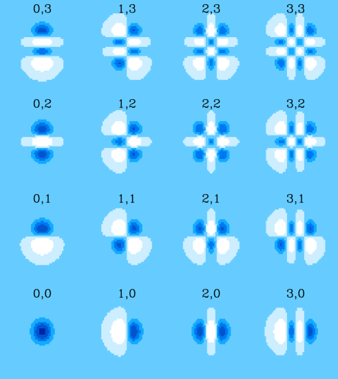
Figure 2: First few 2-dimensional Cartesian basis functions $\phi_{n_{1},n_{2}}$. The dark and light regions correspond to positive and negative values, respectively.

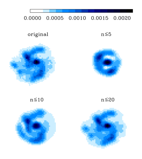
Figure 3: Decomposition of a galaxy image found in the HDF. The original $60\times 60$ pixel HST image (upper left-hand panel) can be compared with the reconstructed images with different maximum order $n=n_{1}+n_{2}$. The shapelet scale is chosen to be $\beta=4$ pixels. The lower right-hand panel ($n\leq 20$) is virtually indistinguishable from the initial image.

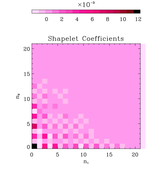
Figure 4: Shapelet coefficients for the image decomposition of the previous figure. Since the coefficient array is sparse, the images can be reconstructed from the few first largest coefficients.

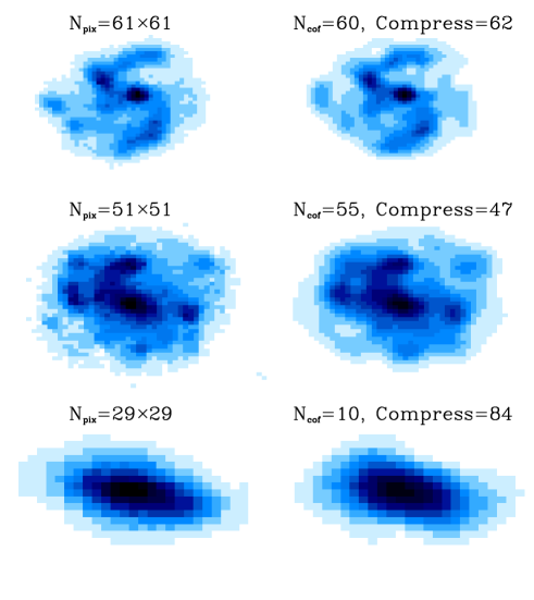
Figure 5: Reconstruction and compression of three HST galaxy images using shapelets. The left-hand column shows the orginal images extracted from the HDF and list $N_{\rm pix}$ their size in pixels. The right-hand column shows their reconstructed image from the $N_{\rm cof}$ largest coefficients (in absolute value) of their shapelet decomposition. Because the coefficient matrix is typically sparse, a large compression factor $N_{\rm pix}/N_{\rm cof}$ is achieved. The shapelet scale was chosen to be $\beta=4$ pixels in all 3 cases.

3.2 Photometry and Astrometry

The most basic quantities to measure for an object image are its total flux (photometry), centroid position (astrometry) and size. Let us first decompose the intensity $f({\mathbf{x}})$ of the object into shapelet coefficients $f_{\mathbf{n}}=\langle{\mathbf{n}};\beta|f\rangle$ as in Equation (22).

Using the integral property of Equation (17), it is then easy to show that the total flux $F\equiv\int d^{2}xf({\mathbf{x}})$ of the object is

$$F=\pi^{\frac{1}{2}}\beta\sum_{n1,n2}^{\rm even}2^{\frac{1}{2}(2-n_{1}-n_{2})}\left(\begin{array}[]{c}n_{1}\\ n_{1}/2\end{array}\right)^{\frac{1}{2}}\left(\begin{array}[]{c}n_{2}\\ n_{2}/2\end{array}\right)^{\frac{1}{2}}f_{n_{1}n_{2}},$$ (26)

where the sum is over even values of $n_{1}$ and $n_{2}$.

Using Equations (17) and (13), one can also show that the centroid of the object $x_{i}^{f}\equiv\int d^{2}xx_{i}f({\mathbf{x}})/F$ is given by

$$x_{1}^{f} = \pi^{\frac{1}{2}}\beta^{2}F^{-1}\sum_{n1}^{{\rm odd}}\sum_{n2}^{{\rm even}}(n_{1}+1)^{\frac{1}{2}}2^{\frac{1}{2}(2-n_{1}-n_{2})}$$ (31)

$$\times\left(\begin{array}[]{c}n_{1}+1\\ (n_{1}+1)/2\end{array}\right)^{\frac{1}{2}}\left(\begin{array}[]{c}n_{2}\\ n_{2}/2\end{array}\right)^{\frac{1}{2}}f_{n_{1}n_{2}},$$

and similarly for $x_{2}^{f}$.

Similarly, the rms radius $r_{f}$ defined by $r_{f}^{2}\equiv\int d^{2}xx^{2}f({\mathbf{x}})/F$ is given by

$$r_{f}^{2} = \pi^{\frac{1}{2}}\beta^{3}F^{-1}\sum_{n1,n2}^{\rm even}2^{\frac{1}{2}(4-n_{1}-n_{2})}\left(1+n_{1}+n_{2}\right)$$ (36)

$$\times\left(\begin{array}[]{c}n_{1}\\ n_{1}/2\end{array}\right)^{\frac{1}{2}}\left(\begin{array}[]{c}n_{2}\\ n_{2}/2\end{array}\right)^{\frac{1}{2}}f_{n_{1}n_{2}},$$

These expressions can be used, by iteration, to find the optimal centre and scale of the basis functions.

3.3 Coordinate Transformations

Let us consider a general coordinate transformation of the form ${\mathbf{x}}\rightarrow{\mathbf{x}}^{\prime}=(1+{\mathbf{\Psi}}){\mathbf{x}}+{\mathbf{\epsilon}}$, where ${\mathbf{\Psi}}$ is a $2\times 2$ matrix, ${\mathbf{\epsilon}}=(\epsilon_{1},\epsilon_{2})$ is a small displacement. Such a transformation can arise for instance from a translation, rotation or from the action of gravitational lensing. We assume that the transformation matrix ${\mathbf{\Psi}}$ and the displacement ${\mathbf{\epsilon}}$ are small and constant across the object. We parametrise the matrix ${\mathbf{\Psi}}$ following the gravitational lensing conventions as

$${\mathbf{\Psi}}=\left(\begin{array}[]{cc}\kappa+\gamma_{1}&\gamma_{2}-\rho\\ \gamma_{2}+\rho&\kappa-\gamma_{1}\\ \end{array}\right),$$ (37)

where $\rho$ describes rotations and the convergence $\kappa$ describes overall dilatations and contractions. The shear $\gamma_{1}$ ($\gamma_{2}$) describes stretches and compressions along (at $45^{\circ}$ from) the x-axis. The displacements $\epsilon_{1}$ and $\epsilon_{2}$ correspond to translations along the $x$ and $y$-axis, respectively.

Under this transformation, the intensity $f({\mathbf{x}})$ of an object becomes

$$f^{\prime}({\mathbf{x}}^{\prime})=f({\mathbf{x}}({\mathbf{x}}^{\prime}))\simeq f({\mathbf{x}}^{\prime}-{\mathbf{\Psi}}{\mathbf{x}}^{\prime}-{\mathbf{\epsilon}}).$$ (38)

Since we are now considering infinitesimal transformations, we can Taylor expand this expression and only keep the terms which are first order in $\Psi$. After using Equations (11) and (13), we find

$$f^{\prime}\simeq(1+\rho\hat{R}+\kappa\hat{K}+\gamma_{j}\hat{S}_{j}+\epsilon_{i}\hat{T}_{i})f,$$ (39)

where $\hat{R}$, $\hat{K}$, $\hat{S}_{i}$ and $\hat{T}_{i}$ are the operators generating rotation, convergence, shears and translations, respectively, and where we have used the Einstein summation convention. The generators are given by

$$\hat{R} = -i\left(\hat{x}_{1}\hat{p}_{2}-\hat{x}_{2}\hat{p}_{1}\right)=\hat{a}_{1}\hat{a}_{2}^{\dagger}-\hat{a}_{1}^{\dagger}\hat{a}_{2}$$

$$\hat{K} = -i\left(\hat{x}_{1}\hat{p}_{1}+\hat{x}_{2}\hat{p}_{2}\right)=1+\frac{1}{2}\left(\hat{a}_{1}^{\dagger 2}+\hat{a}_{2}^{\dagger 2}-\hat{a}_{1}^{2}-\hat{a}_{2}^{2}\right)$$

$$\hat{S}_{1} = -i\left(\hat{x}_{1}\hat{p}_{1}-\hat{x}_{2}\hat{p}_{2}\right)=\frac{1}{2}\left(\hat{a}_{1}^{\dagger 2}-\hat{a}_{2}^{\dagger 2}-\hat{a}_{1}^{2}+\hat{a}_{2}^{2}\right)$$

$$\hat{S}_{2} = -i\left(\hat{x}_{1}\hat{p}_{2}+\hat{x}_{2}\hat{p}_{1}\right)=\hat{a}_{1}^{\dagger}\hat{a}_{2}^{\dagger}-\hat{a}_{1}\hat{a}_{2}$$

$$\hat{T}_{j} = -i\hat{p}_{j}=\frac{1}{\sqrt{2}}(\hat{a}_{j}^{\dagger}-\hat{a}_{j}),~{}~{}~{}j=1,2.$$ (40)

The rotation generator $\hat{R}$ is thus simply equal to the angular momentum operator in 2-dimensions

$$\hat{L}=\hat{x}_{1}\hat{p}_{2}-\hat{x}_{2}\hat{p}_{1}=i\left(\hat{a}_{1}\hat{a}_{2}^{\dagger}-\hat{a}_{1}^{\dagger}\hat{a}_{2}\right),$$ (41)

up to a factor of $-i$. Similarly, the translation generator $\hat{T}_{i}$ is simply equal to the the linear momentum operator $\hat{p}_{i}$, up to the same factor.

These expressions along with Equation (14) make it easy to compute the effect of these transformations on the basis functions $B_{\mathbf{n}}$. For instance, the generator of translations along the $x$-axis has a matrix representation $T_{1{\mathbf{m}n}}\equiv\langle{\mathbf{m}}|\hat{T}_{1}|{\mathbf{n}}\rangle$ given by

$$T_{1{\mathbf{m}n}}=\frac{1}{\sqrt{2}}\left[\sqrt{n_{1}}\delta_{m_{1},n_{1}-1}-\sqrt{n_{1}+1}\delta_{m_{1},n_{1}+1}\right]\delta_{m_{2},n_{2}},$$ (42)

and similarly for the other generators.

The meaning of the generators can be seen by studying their action on the ground state. For instance, it is easy to see that under the action of a shear $\gamma_{1}$, the ground state $|00\rangle$ becomes

$$|00\rangle^{\prime}\simeq(1+\gamma_{1}\hat{S}_{1})|00\rangle=|00\rangle+\frac{\gamma_{1}}{\sqrt{2}}\left[|20\rangle-|20\rangle\right].$$ (43)

The action of the different transformations on the ground states can be calculated in the same way and are shown in Figure 6. Clearly, their action is as expected from their definition. Since the ground state is circularly symmetric, the rotation operator vanishes when applied to $|00\rangle$, i.e. $\hat{R}|00\rangle=0$. More instructively, we can consider the effect of $\hat{R}$ on an asymmetric state like $|10\rangle$. It is also shown in the bottom row of the figure. As expected the state $|10\rangle$ is rotated counter-clockwise by the rotation operator.

Finite transformations can be produced by exponentiating the generators. For instance, after a finite rotation by an angle $\rho$ the function $f$ becomes

$$f^{\prime}=e^{\rho\hat{R}}f=\left(\sum_{n=0}^{\infty}\frac{(\rho\hat{R})^{n}}{n!}\right)f,$$ (44)

and similarly for the shear and convergence.

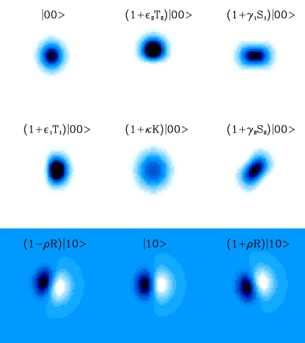
Figure 6: Effect of coordinate transformations on the first two shapelet states $|00\rangle$ and $|10\rangle$. All coordinate transformations are considered: translations, rotations, convergence and shear. They are parametrised by $\epsilon_{i}$, $\rho$, $\kappa$ and $\gamma_{i}$, respectively, which were all assigned a value of 0.3 for the purpose of this figure. Their action on any state are easily calculated using the raising and lowering operators $\hat{a}_{i}^{\dagger}$ and $\hat{a}_{i}$. Clearly, the different transformation generators act as expected from their definition.

3.4 Effect of Noise

In this section, we study the uncertainty induced by noise on the basis function decomposition, in the case of correlated and uncorrelated background noise, and of Poisson noise. The observed intensity of an object is

$$f^{\prime}({\mathbf{x}})=f({\mathbf{x}})+n({\mathbf{x}}),$$ (45)

where $f({\mathbf{x}})$ is the intrinsic intensity of the object and $n({\mathbf{x}})$ is the noise. The noise is taken to be unbiased, so that $\langle n({\mathbf{x}})\rangle=0$ and is characterised by its correlation function $\eta({\mathbf{x}},{\mathbf{x}}^{\prime})\equiv\langle n({\mathbf{x}})n({\mathbf{x}}^{\prime})\rangle$. Here the brackets refer to an ensemble average over noise realisations.

The observed basis coefficients are then $f^{\prime}_{{\mathbf{k}}}=\langle{\mathbf{k}},\beta|f^{\prime}\rangle$ and are unbiased, i.e.

$$\langle f^{\prime}_{{\mathbf{k}}}\rangle=f_{{\mathbf{k}}},$$ (46)

where $f_{{\mathbf{k}}}=\langle{\mathbf{k}},\beta|f\rangle$ are the intrinsic coefficients. It is then easy to show that the covariance matrix ${\rm cov}[f^{\prime}_{{\mathbf{k}}},f^{\prime}_{{\mathbf{l}}}]\equiv\langle(f^{\prime}_{{\mathbf{k}}}-\langle f^{\prime}_{{\mathbf{k}}}\rangle)(f^{\prime}_{{\mathbf{l}}}-\langle f^{\prime}_{{\mathbf{l}}}\rangle)\rangle$ for the observed coefficients is given by

$${\rm cov}[f^{\prime}_{{\mathbf{k}}},f^{\prime}_{{\mathbf{l}}}]=\int d^{2}x\int d^{2}x^{\prime}~{}B_{k}({\mathbf{x}},\beta)\eta({\mathbf{x}},{\mathbf{x}}^{\prime})B_{l}({\mathbf{x}},\beta).$$ (47)

To be more specific, we first consider the case of homogeneous background noise, as can be produced by sky or instrumental backgrounds. If the background noise is uncorrelated, $\eta({\mathbf{x}})=\sigma_{n}^{2}\delta^{(2)}({\mathbf{x}})$, where $\sigma_{n}$ is the rms noise. As a result, the covariance matrix reduces to

$${\rm cov}[f^{\prime}_{{\mathbf{k}}},f^{\prime}_{{\mathbf{l}}}]=\sigma_{n}^{2}\delta_{lk},$$ (48)

where we have used the orthonormality of the basis functions (Eq. [4]). In this case, the covariance matrix is thus diagonal, so that each coefficient is statistically independent. Moreover, the diagonal elements are all equal. Uncorrelated noise thus populates each coefficient equally, and is thus “white” as in the case of Fourier transforms.

In the case of spatially correlated but homogeneous noise, the noise correlation function is only a function of separation and can thus be written as $\eta({\mathbf{x}}-{\mathbf{x}}^{\prime})$. As a result, Equation (47) reduces to the integral of a convolution and can thus be written symbolically as

$${\rm cov}[f^{\prime}_{{\mathbf{k}}},f^{\prime}_{{\mathbf{l}}}]=\langle{\mathbf{k}},\beta|\eta*({\mathbf{l}},\beta)\rangle,$$ (49)

in the notation of Equation (53). A convenient way to evaluate this is to decompose $\eta({\mathbf{x}})$ itself into basis functions and then to use the results of §4 below. Spatial correlations in the noise thus produces correlations in the coefficients.

Another case of practical interest is that in which the noise is dominated by Poisson shot noise. If the intensities are measured in units of photon counts, the noise correlation function is then $\eta({\mathbf{x}},{\mathbf{x}}^{\prime})=f({\mathbf{x}})\delta^{(2)}({\mathbf{x}}-{\mathbf{x}}^{\prime})$. As a result, the covariance matrix is

$${\rm cov}[f^{\prime}_{{\mathbf{k}}},f^{\prime}_{{\mathbf{l}}}]=\sum_{{\mathbf{m}}}f_{{\mathbf{m}}}B^{(3)}_{{\mathbf{k}},{\mathbf{l}},{\mathbf{m}}},$$ (50)

where $B^{(3)}_{{\mathbf{k}},{\mathbf{l}},{\mathbf{m}}}(\beta,\beta,\beta)$ is the 3-product integral defined in Equation (55) below, and which is evaluated analytically in Paper II. In this case again, the covariance coefficient is made non-diagonal by the noise correlation, but is easily calculable analytically.

4 Convolution

We now show how shapelets behave under convolutions, an operation which often occurs in practice (eg. under the action of PSF, seeing, smoothing, etc). We start by considering convolution by a general kernel in 1-dimensions, and then study the special case of smoothing by a gaussian. Finally, we treat the 2-dimensional case, and illustrate the results with the example of an HST galaxy image.

4.1 Convolution in 1-Dimension

Let us first consider the convolution of two arbitrary 1-dimensional functions $f(x)$ and $g(x)$. Their convolution $h(x)$ can be written as

$$h(x)\equiv(f*g)(x)\equiv\int_{-\infty}^{\infty}dx^{\prime}~{}f(x-x^{\prime})g(x^{\prime})$$ (51)

Each function can be decomposed into our basis functions with scales $\alpha$, $\beta$ and $\gamma$. These scales are chosen to be most convenient in each case. The coefficients are then $f_{n}\equiv\langle n;\alpha|f\rangle$, $g_{n}\equiv\langle n;\beta|g\rangle$, $h_{n}\equiv\langle n;\gamma|h\rangle$. Our aim is to find an expression which relates $h_{n}$ to $f_{n}$ and $g_{n}$. Since convolution is a bi-linear operation, this relation will be of the form

$$h_{n}=\sum_{m,l=0}^{\infty}C_{nml}f_{m}g_{l},$$ (52)

where the convolution tensor can be written symbolically as

$$C_{nml}(\gamma,\alpha,\beta)\equiv\langle n;\gamma|(m;\alpha)*(l;\beta)\rangle$$ (53)

and is a function of the scale lengths. Using the properties of the basis functions under Fourier transforms (Eq. [9]), it is easy to show that the convolution tensor is given by

$$C_{nml}(\gamma,\alpha,\beta)=(2\pi)^{\frac{1}{2}}(-1)^{n}i^{n+m+l}B^{(3)}_{nml}(\gamma^{-1},\alpha^{-1},\beta^{-1}),$$ (54)

where the 3-product integral is $B^{(3)}_{nml}(a_{1},a_{2},a_{3})$ is defined as

$$B^{(3)}_{lmn}(a_{1},a_{2},a_{3})\equiv\int_{-\infty}^{\infty}dx~{}B_{l}(x,a_{1})B_{m}(x,a_{2})B_{n}(x,a_{3}).$$ (55)

As we show in Paper II, this integral can be easily evaluated analytically with a recurrence relation.

4.2 Smoothing in 1-Dimension

The special case consisting of smoothing by a gaussian is useful in practice. In this case, we let

$$g(x)\equiv(2\pi)^{-\frac{1}{2}}\beta^{-1}e^{-\frac{x^{2}}{2\beta^{2}}},$$ (56)

which is normalised so that $\int dx~{}g(x)=1$. We can then write the coefficients for the smoothed function $h(x)$ as

$$h_{n}=\sum_{m}G_{nm}f_{m},$$ (57)

where $G_{nm}(\gamma,\alpha,\beta)=\sum_{l}C_{nml}(\gamma,\alpha,\beta)g_{l}$ is the smoothing matrix. The gaussian $g(x)$ can be thought as a (non-normalised) $n=0$ shapelet state of amplitude $g_{0}=\langle 0;\beta|g\rangle$, so that $G_{nm}=C_{nm0}g_{0}$. Using the generating function for Hermite polynomials, one can show that, for the natural choice of $\gamma^{2}=\alpha^{2}+\beta^{2}$, the smoothing matrix is given by

$$G_{nm}=2^{\frac{n-m}{2}}\left(\frac{\omega}{\beta}\right)^{\frac{1}{2}}\frac{\omega^{m}}{\beta^{n}\alpha^{m-n}}\frac{(m!/n!)^{\frac{1}{2}}}{\left(\frac{m-n}{2}\right)!},$$ (58)

for $m-n\geq 0$ and even ($G_{nm}$ vanishes otherwise), and where $\omega^{-2}\equiv\alpha^{-2}+\beta^{-2}$.

Figure 7 shows how this analytic formula can be used to efficiently smooth a 2-dimensional image (see discussion in §4.3 below). An intuitive feeling for the effect of convolution on the shapelet coefficients can be obtained from Figure 8, which graphically shows the smoothing matrix $G_{nm}(\alpha,\beta,\gamma=(\alpha^{2}+\beta^{2})^{\frac{1}{2}})$ for different values of the smoothing scale $\beta$. As expected, the smoothing matrix approaches the identity matrix in the limit of vanishing smoothing scale ($\beta\rightarrow 0$). On the other hand, for very large smoothing kernels ($\beta\rightarrow\infty$) it reduces to a projection of all the input modes $m$ onto the $n=0$ output mode. For intermediate scales, the smoothing matrix takes the form of a band which rotates from the vertical to the horizontal as the smoothing scale $\beta$ is increased. Smoothing thus corresponds to a projection of the input modes into output modes of smaller order. The high-order modes indeed have oscillations on small scales and are thus gradually lost when we increase the smoothing scale $\beta$.

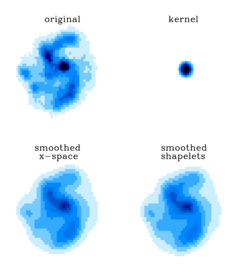
Figure 7: Illustration of smoothing in Shapelet Space. The original galaxy image ($61\times 61$ pixels) of Figure 3 (shown again in the upper-left panel) is smoothed with a gaussian kernel with standard deviation $\beta=2$ pixels (upper-right panel). The resulting image smoothed using shapelets (lower-right panel) is almost indistinguishable from that smoothed using direct convolution in real-space (lower-left panel). In shapelet space, smoothing is a simple matrix multiplication and can be very efficient when the coefficient matrix is sparse, as is the case here (see Figure  4).

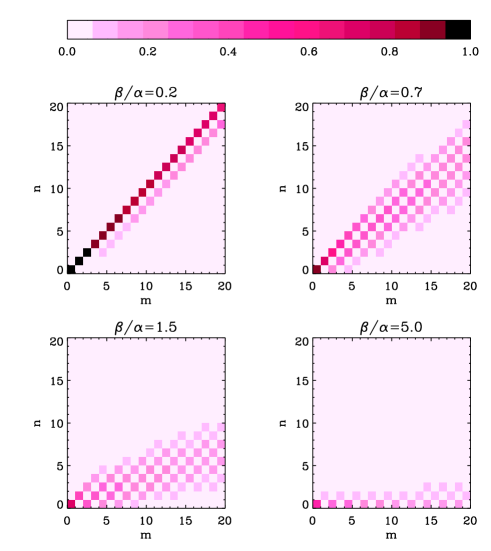
Figure 8: Graphical representation of the smoothing matrix $|G_{nm}|$ for different size $\beta$ of the smoothing kernel (in units of the input shapelet scale $\alpha$). The horizontal axis corresponds to the input (unsmoothed) mode $m$, while the vertical axis shows the output (smoothed) mode $n$. For small smoothing scales ($\beta\rightarrow 0$) the smoothing matrix approaches the identity matrix (upper-left panel). For large smoothing scales ($\beta\rightarrow\infty$), it approaches a projection onto the $n=0$ mode (lower-right panel). For intermediate values, it corresponds to a projection onto lower order modes (upper-right and lower-left panels).

4.3 Convolution in 2-Dimensions

Let us now consider the convolution of two 2-dimensional functions, such as

$$h({\mathbf{x}})=(f*g)({\mathbf{x}})=\int d^{2}x~{}f({\mathbf{x}}-{\mathbf{x}}^{\prime})g({\mathbf{x}}^{\prime}).$$ (59)

We again first decompose each function into shapelet coefficients $f_{\mathbf{n}}\equiv\langle{\mathbf{n}};\alpha|f\rangle$, $g_{\mathbf{n}}\equiv\langle{\mathbf{n}};\beta|g\rangle$, and $h_{\mathbf{n}}\equiv\langle{\mathbf{n}};\gamma|h\rangle$ with shapelet scales $\alpha$, $\beta$ and $\gamma$ respectively, and where ${\mathbf{n}}=(n_{1},n_{2})$ as before. Because convolution is bilinear we can again relate the convolved to the unconvolved coefficients by

$$h_{\mathbf{n}}=\sum_{{\mathbf{m}},{\mathbf{l}}}C_{{\mathbf{n}},{\mathbf{m}},{\mathbf{l}}}f_{\mathbf{m}}g_{\mathbf{l}}$$ (60)

where $C_{{\mathbf{n}},{\mathbf{m}},{\mathbf{l}}}(\gamma,\alpha,\beta)$ is the 2-dimensional convolution tensor. From the separability of the 2-dimensional basis functions (see Eq. [18), it is easy to show that this tensor is equal to

$$C_{{\mathbf{n}},{\mathbf{m}},{\mathbf{l}}}(\gamma,\alpha,\beta)=C_{n_{1},m_{1},l_{1}}(\gamma,\alpha,\beta)C_{n_{2},m_{2},l_{2}}(\gamma,\alpha,\beta),$$ (61)

where the tensors appearing on the right-hand side are the 1-dimensional convolution tensor defined in Equation (54).

We can also consider the special case of smoothing with a 2-dimensional gaussian. In this case, $g({\mathbf{x}})=(2\pi\beta^{2})^{-1}e^{-\frac{x^{2}}{2\beta^{2}}}$, which is normalised so that $\int d^{2}x~{}g({\mathbf{x}})=1$. The smoothed coefficients are then given by

$$h_{\mathbf{n}}=\sum_{{\mathbf{m}}}G_{{\mathbf{n}},{\mathbf{m}}}f_{{\mathbf{m}}},$$ (62)

where $G_{{\mathbf{n}},{\mathbf{m}}}(\gamma,\alpha,\beta)$ is the 2-dimensional smoothing matrix. It is again easy to show that it is equal to

$$G_{{\mathbf{n}},{\mathbf{m}}}(\gamma,\alpha,\beta)=G_{n_{1},m_{1}}(\gamma,\alpha,\beta)G_{n_{2},m_{2}}(\gamma,\alpha,\beta),$$ (63)

in terms of the 1-dimensional smoothing matrix defined in §4.2. With the natural choice $\gamma^{2}=\alpha^{2}+\beta^{2}$, it can be evaluated using Equation (58).

Figure 7 shows the how the galaxy image of Figure 3 can be smoothed using our shapelet method. The resulting image is indistinguishable from that derived using ordinary convolution in real-space (also shown). The shapelet method is however computationally very efficient when the coefficient matrix is sparse as is the case here (see Figure 4). The effect of smoothing on the shapelet coefficients of this galaxy can be seen in Figure 9. For clarity, the smoothing scale was enhanced to $\beta=4$ pixels. Clearly, convolution amounts to a projection onto the lower order states, as discussed in §4.2.

Figure 9: Shapelet coefficients of the same galaxy (Figure 3) after smoothing with a gaussian kernel. For clarity, the standard deviation of the kernel was increased to $\beta=4$ pixels. By comparing this distribution with that before smoothing (Figure 4), it is easy to see how convolution amounts to a projection onto the lower order shapelet states.

5 Polar Shapelets

The cartesian basis functions discussed above are separable in the cartesian coordinates $x_{1}$ and $x_{2}$. It is also useful to construct basis functions which are separable in the polar coordinates $x$ and $\varphi$. These are eigenstates of the Hamiltonian $\hat{H}$ and of the angular momentum $\hat{L}$ simultaneously, and thus have a number of convenient features. In this section, we show how they can be constructed and study some of their properties.

5.1 Raising and Lowering Operators

To construct the polar basis functions, we first define the left and right lowering operators as (see eg. Cohen-Tannoudji et al. 1977)

$$\hat{a}_{l}=\frac{1}{\sqrt{2}}\left(\hat{a}_{1}+i\hat{a}_{2}\right),~{}~{}\hat{a}_{r}=\frac{1}{\sqrt{2}}\left(\hat{a}_{1}-i\hat{a}_{2}\right).$$ (64)

The associated raising operators are $\hat{a}_{l}^{\dagger}$ and $\hat{a}_{r}^{\dagger}$, respectively. The only non-vanishing commutators between these operators are

$$[\hat{a}_{l},\hat{a}_{l}^{\dagger}]=[\hat{a}_{r},\hat{a}_{r}^{\dagger}]=1.$$ (65)

The Hamiltonian (Eq. [21]) and angular momentum (Eq. [41]) operators for the 2-dimensional QHO can be then be written as

$$\hat{H}=\hat{N}_{r}+\hat{N}_{l}+1,~{}~{}~{}\hat{L}=\hat{N}_{r}-\hat{N_{l}},$$ (66)

where the left-handed and right-handed number operators are naturally defined as

$$\hat{N}_{l}=\hat{a}_{l}^{\dagger}\hat{a}_{l},~{}~{}~{}\hat{N}_{r}=\hat{a}_{r}^{\dagger}\hat{a}_{r}.$$ (67)

The operators $\hat{a}_{l}^{\dagger}$, $\hat{a}_{r}^{\dagger}$, $\hat{a}_{l}$, and $\hat{a}_{r}$ can thus be thought of as creating and destroying left- and right-handed quanta.

5.2 Angular Momentum States

Since the operators $\hat{N}_{r}$ and $\hat{N_{l}}$ form a complete set of commuting observables, their eigenstates $|n_{l},n_{r}\rangle$ provide a complete basis for our function space. These states are defined $\hat{N}_{l}|n_{l},n_{r}\rangle=n_{l}|n_{l},n_{r}\rangle$, and similarly for $\hat{N}_{r}$, for $n_{l}$ $n_{r}$ non-negative integers. They can be constructed by applying the raising operators several times on the ground state $|n_{1}=0,n_{2}=0\rangle=|n_{l}=0,n_{r}=0\rangle\equiv|0,0\rangle$, as

$$|n_{r},n_{l}\rangle=\frac{(\hat{a}_{r}^{\dagger})^{n_{r}}(\hat{a}_{l}^{\dagger})^{n_{l}}}{\sqrt{n_{r}!n_{l}!}}|0,0\rangle.$$ (68)

From Equation (66), it is easy to see that

$$\hat{H}|n_{l},n_{r}\rangle=(n_{r}+n_{l})|n_{l},n_{r}\rangle,~{}~{}\hat{L}|n_{l},n_{r}\rangle=(n_{r}-n_{l})|n_{l},n_{r}\rangle.$$ (69)

We can therefore relabel these states in terms of their energy and angular momentum quantum numbers, $n=n_{r}+n_{l}$ and $m=n_{r}-n_{l}$, as

$$|n,m\rangle=|n_{l}=\frac{1}{2}(n-m),n_{r}=\frac{1}{2}(n+m)\rangle.$$ (70)

The angular momentum quantum number takes on the $n+1$ values given by $m=-n,-n+2,\ldots,n-2,n$.

5.3 Basis Functions

Using the $x$-representation of $\hat{a}_{l}^{\dagger}$ and $\hat{a}_{r}^{\dagger}$, one can show that the basis functions $\chi_{n_{l},n_{r}}(x,\varphi)\equiv\langle x|n_{l},n_{r}\rangle$ for the angular momentum states are given by

$$\chi_{n_{l},n_{r}}(x,\varphi)=\left[\pi n_{l}!n_{r}!\right]^{-\frac{1}{2}}H_{n_{l},n_{r}}(x)e^{-x^{2}/2}e^{i(n_{r}-n_{l})\varphi},$$ (71)

where $H_{n_{k},n_{r}}(x)$ are polynomials, which we call ‘polar Hermite polynomials’. They can be computed by noting that $H_{0,0}(x)=1$ and by using the recursion relation

$$\frac{l-k}{x}H_{k,l}(x)=lH_{k,l-1}-kH_{k-1,l}.$$ (72)

The diagonal polynomials can be computed using

$$H_{kk}=H_{k+1,k-1}-x^{-1}H_{k,k-1}.$$ (73)

The first few polar Hermite polynomials are listed in Table 1. They have a number of useful properties. In particular, they are symmetric, i.e. $H_{k,l}=H_{l,k}$ and their derivative obey

$$H^{\prime}_{k,l}(x) = kH_{k-1,l}(x)+lH_{k,l-1}(x)$$ (74)

$$= 2xH_{k,l}(x)-H_{k+1,l}-H_{k,l+1}.$$

Dimensional polar basis functions can be constructed as

$$A_{n_{l},n_{r}}(x,\varphi;\beta)=\beta^{-1}\chi_{n_{l},n_{r}}(\beta^{-1}x,\varphi).$$ (75)

It is easy to check that these are orthonormal, i.e. that

$$\int_{0}^{2\pi}d\varphi\int_{0}^{\infty}dx~{}xA_{n_{l},n_{r}}(x,\varphi;\beta)A_{n_{l}^{\prime},n_{r}^{\prime}}(x,\varphi;\beta)$$

$$=\langle{n_{l},n_{r};\beta}|{n_{l}^{\prime},n_{r}^{\prime};\beta}\rangle=\delta_{n_{l},n_{l}^{\prime}}\delta_{n_{r},n_{r}^{\prime}}.$$ (76)

The radial dependence $|\chi_{n_{l},n_{r}}(x)|$ of the first few polar shapelet functions is shown in Figure 10.

Table 1: First few polar Hermite polynomials

$H_{0,0}(x)=1$

$H_{0,1}(x)=H_{1,0}(x)=x$

$H_{0,2}(x)=H_{2,0}(x)=x^{2}$

$H_{1,1}(x)=x^{2}-1$

$H_{0,3}(x)=H_{3,0}(x)=x^{3}$

$H_{1,2}(x)=H_{2,1}(x)=x^{3}-2x$

$H_{0,4}(x)=H_{4,0}(x)=x^{4}$

$H_{1,3}(x)=H_{3,1}(x)=x^{4}-3x^{2}$

$H_{2,2}(x)=x^{4}-4x^{2}+2$

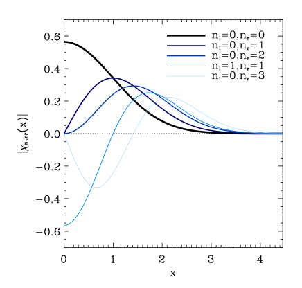
Figure 10: Radial dependence of the first few polar basis functions $|\chi_{n_{l},n_{r}}(x)|$.

5.4 Relation to Cartesian States

It is useful to relate the angular momentum states $|n,m\rangle$ to the cartesian states $|n_{1},n_{2}\rangle$. Using Equations (64) and (68) along with the binomial expansion, one can show that the transformation matrix between these two bases is given by

$$\langle n_{1},n_{2}|n_{l},n_{r}\rangle = 2^{-\frac{1}{2}(n_{r}+n_{l})}i^{n_{r}-n_{l}}\left[\frac{n_{1}!n_{2}!}{n_{r}!n_{l}!}\right]^{\frac{1}{2}}\delta_{n_{1}+n_{2},n_{r}+n_{l}}$$ (81)

$$\sum_{n_{r}^{\prime}=0}^{n_{r}}\sum_{n_{l}^{\prime}=0}^{n_{l}}i^{n_{l}^{\prime}-n_{r}^{\prime}}\left(\begin{array}[]{c}n_{r}\\ n_{r}^{\prime}\end{array}\right)\left(\begin{array}[]{c}n_{l}\\ n_{l}^{\prime}\end{array}\right)\delta_{n_{r}^{\prime}+n_{l}^{\prime},n_{1}}.$$

This shows that only states with $n_{1}+n_{2}=n_{r}+n_{l}$ are mixed. The first few $|n,m\rangle$ states are given in terms of $|n_{1}n_{2}\rangle$ states in Table 2.

Table 2: Angular momentum states $|n,m\rangle$ in terms of the cartesian states $|n_{1},n_{2}\rangle$.

$|n=0,m=0\rangle=|0,0\rangle$

$|n=1,m=1\rangle=\frac{1}{\sqrt{2}}\left[|1,0\rangle+i|0,1\rangle\right]$

$|n=1,m=-1\rangle=\frac{1}{\sqrt{2}}\left[|1,0\rangle-i|0,1\rangle\right]$

$|n=2,m=2\rangle=\frac{1}{2}\left[|2,0\rangle+i\sqrt{2}|1,1\rangle-|0,2\rangle\right]$

$|n=2,m=0\rangle=\frac{1}{\sqrt{2}}\left[|2,0\rangle+|0,2\rangle\right]$

$|n=2,m=-2\rangle=\frac{1}{2}\left[|2,0\rangle-i\sqrt{2}|1,1\rangle-|0,2\rangle\right]$

5.5 Properties

Because the polar shapelet states are eigenstates of the angular momentum, they have simple rotational properties. Indeed, under a finite rotation by an angle $\rho$, the polar states transform as

$$|n_{r},n_{l}\rangle^{\prime}=e^{-i\rho\hat{L}}|n_{r},n_{l}\rangle=e^{-i\rho(n_{r}-n_{l})}|n_{r},n_{l}\rangle,$$ (82)

where we have used the exponentiation (Eq. [44]) of the rotation generator $\hat{R}=-i\hat{L}$ (Eq. [3.3]) to operate a finite rotation. In this basis, finite rotations thus corresponds only to a phase factor.

It is therefore a simple matter to rotate an arbitrary function $f({\mathbf{x}})$. First, we decompose it into polar shapelet coefficients $f_{n_{r},n_{l}}=\langle n_{r},n_{l};\beta|f\rangle$, with an appropriate shapelet scale $\beta$. The coefficients $f_{n_{r},n_{l}}^{\prime}=\langle n_{r},n_{l};\beta|f^{\prime}\rangle$ of the rotated function $f^{\prime}({\mathbf{x}})$ are then given simply by

$$f^{\prime}_{n_{r},n_{l}}=e^{-i(n_{r}-n_{l})\rho}f_{n_{r},n_{l}}.$$ (83)

By contrast, operating a finite rotation in the cartesian basis requires an infinite number of applications of the $\hat{R}$ operator (see Eq. [44]) and is thus impractical. On the other hand, convolutions do not have simple analytical expressions in the polar basis, as they do in the cartesian basis (see §4 and Paper II). The results of §5.4, can thus be conveniently used to convert from one basis to the other, depending on the operation to be performed.

6 Applications

Now that we have developed the main formalism for shapelets, we illustrate the method using images from the Hubble Space Telescope (HST). We also discuss several direct applications of shapelets.

6.1 Example with HST images

As an example, we apply the shapelet decomposition method to images of galaxies found in the Hubble Deep Field (HDF; Williams et al. 1996), the deepest images observed with the Hubble Space telescope (HST). Figure 3 shows the original $61\times 61$ image $f({\mathbf{x}})$ of one such galaxy (upper-left hand panel). Using Equation (22), we first compute the shapelet coefficients $f_{\mathbf{n}}$ of the galaxy with a shapelet scale $\beta=4$ pixels. We then reconstruct the image using Equation (23) including coefficients up to a maximum order $n_{1}+n_{2}\leq n_{\rm max}$. The resulting reconstructed images are shown on the figure for different values of $n_{\rm max}$. As $n_{\rm max}$ is increased, more small scale and large scale features are recovered, as expected from the properties of our basis functions (see §2.4). For $n_{\rm max}=20$, the reconstructed image is almost indistinguishable from the original.

Figure 4 gives a graphical representation of the shapelet coefficient matrix $f_{n_{1},n_{2}}$ for this image. This can be thought as the representation of the galaxy in ‘shapelet space’. As is apparent on the figure, the coefficient matrix is rather sparse. The fact that the odd coefficients are small results from the fact that the shapelet center was chosen to be close to the centroid of the galaxy. The coefficients are negligibly small beyond $n_{1}+n_{2}\ga 15$, thus explaining why we obtain a virtually full reconstruction with $n_{\rm max}=20$.

Because of the sparse nature of the coefficient matrix, we can hope to recover the image from only the first few largest coefficients. Figure 5 shows the reconstruction of the galaxy of Figure 3 and of two other HDF galaxies, by keeping only the $N_{\rm cof}$ coefficients with largest absolute value $|f_{\mathbf{n}}|$. As can be seen from the top two panels, the galaxy image can be faithfully recovered with the top $N_{\rm cof}=60$ coefficients, yielding a compression factor $N_{\rm pix}/N_{\rm cof}$ of 62 compared to the original image which contained $N_{\rm pix}=61\times 61=3721$ pixels. (The bookeeping required to keep track of selected coefficients only requires 1 bit per coefficient, and thus results only in a small overhead relatively to this compression factor). For the other two galaxies shown in the middle and bottom rows, compression factors of about 40-90 are achieved. Note that the galaxy in the bottom row has a simpler structure and thus affords more compression.

6.2 Catalogue Archival

We have seen above that the first few shapelet coefficients capture most of the structure of galaxy images and thus allow strong data compressions. This can be very useful for upcoming and future large galaxy surveys such as the Sloan Digital Sky Survey (SDSS; Gunn & Weinberg 1995), or that derived from the planned SNAP mission (Perlmutter et al. 2001). One can imagine storing the first few shapelet coefficients in the catalog, thus both saving storage and conveying compactly the shape information of each each galaxy. The flux, centroid, major and minor axes and position angle of each galaxy could then be computed from their shapelet coefficients directly (as described in §3.2), thus avoiding the need to consider several definitions of magnitudes. Since galaxy shapes in different wavelengths are strongly correlated, the treatment of multi-colour data could be done efficiently by decomposing differences of the images in different pass-bands and again keeping the largest coefficients. The resulting catalogue could then also be useful for study of galaxy morphology and classification in shapelet space.

6.3 Modeling the Point-Spread Function

Several astronomical techniques (eg. high-precision astrometry and photometry, microlensing, weak lensing, supernova searches, etc) require correction for the Point-Spread Function (PSF) of the telescope across an image. For instance, Alard & Lupton (1998) have developed a technique to take the difference of two images convolved with a spatially varying PSF. Shapelets provide a convenient correction method for the PSF: the PSF shape can be measured at different positions in the field using bright stars and then decomposed into shapelet coefficients; a 2-dimensional polynomial fit for each shapelet coefficient as a function of position can then be performed to derive a model of the PSF shape at any point (Cf. Alard & Lupton 1998 and Kaiser 2000 who used this approach with other sets of basis functions). The convolution matrix can then be inverted to compute the shapelet coefficients of objects prior to convolution. As discussed in §4, convolution amounts to a projection onto lower shapelet order. As a result only low order coefficients can be recovered. Another approach consist of fitting the deconvolved shapelet coefficients convolved to the PSF model to the data (Cf. Kuijken 2000). The analytical properties of shapelets under convolution (see §4 and Paper II) greatly facilitate and clarify the procedure. A detailed study of deconvolution using shapelets will be presented in Paper II.

6.4 Gravitational Lensing

Gravitational Lensing is a powerful method to directly probe the mass of astrophysical objects. In particular, the weak coherent distortions induced by lensing on the images of background galaxies provide a direct measure of the distribution of mass in the Universe. This weak lensing method is now routinely used to study galaxy clusters, and has recently been detected in the field (see reviews by Mellier 1999; Bartelmann & Schneider; Mellier et al. 2000). Because the lensing effect is only of a few percent on large scales, a precise method for measuring the shear is required. The original methods of Bonnet & Mellier (1995) and of Kaiser, Squires & Broadhurst (KSB; 1995) are not sufficiently accurate and stable for the upcoming weak lensing surveys. Thus, several new methods have been proposed (Kuijken 1999; Rhodes, Refregier & Groth 2000; Kaiser 2000). As we briefly describe below, the remarkable properties of our basis functions, make shapelets particularly well suited for providing the basis of a new method.

Let us consider a galaxy with an unlensed intensity $f({\mathbf{x}})$. We have shown in §3.3 that under the action of a weak shear $\gamma_{i}$, the lensed intensity is

$$f^{\prime}\simeq(1+\gamma_{i}\hat{S}_{i})f.$$ (84)

After decomposing these intensities into our basis functions $B_{{\mathbf{n}}}({\mathbf{x}},\beta)$ (Eq. [22]), this becomes a relation between the lensed and the unlensed coefficients given by

$$f^{\prime}_{{\mathbf{n}}}=(\delta_{nm}+\gamma_{i}S_{i{\mathbf{m}n}})f_{{\mathbf{m}}},$$ (85)

where $S_{i{\mathbf{m}n}}\equiv\langle{\mathbf{m}}|\hat{S}_{1}|{\mathbf{n}}\rangle$ is the shear generator matrix given in Equation (3.3). The goal for weak lensing is to estimate the shear from the shapes of an ensemble of galaxies which are assumed to be randomly oriented prior to lensing. In the widely used KSB method, this is done by considering the effect of lensing on the Gaussian-weighted quadrupole moments of the galaxy images. These are exactly equal to the $n_{1}+n_{2}=2$ coefficients in our shapelet decomposition. In as sense, our method thus generalises this approach and capture all the available shape information of galaxies. Because the shear matrix is simple in our cartesian basis, we can then construct an estimator for the shear by comparing the distribution of the lensed shapelet coefficients $f_{\mathbf{n}}^{\prime}$ to that of a training set $f_{\mathbf{n}}$ for which lensing is known to be negligible. This can be done either by constructing a linear shear estimator from the observed coefficients or by using a Maximum Likelihood technique. In Paper II, we follow the first approach and show that shapelets can be used to derive precise shear recovery in realistic simulations of deep optical images (see Bacon et al. 2001).

As Luppino & Kaiser (1997) discussed, the shear acts, in practice, after the smearing produced by the PSF. To account for this, we can first model the PSF across the field, as described in §6.3. Then one of the methods mentioned in this section can be used to derive the deconvolved coefficients from the observed convolved ones. Again, a detailed study of this deconvolution method and its impact in weak lensing measurement will be presented in Paper II.

Shapelets can also be used for strong lensing applications, such as the modeling of cluster or galaxy potentials using multiple images and giant arcs. In §3.3, we concentrated mainly on first order distortions, but also mentioned that distortions of arbitrary amplitudes can be derived by exponentiating the shear and convergence operators (see Eq. [44]). An equivalent method to compute the effect of large distortions on the shapelet coefficients is to use the analytical expression for rescaling of Appendix A. One can then model the shape of the lensed object using shapelets and explore a large class of lens models efficiently by computing the lensed image coefficients analytically. Another possibility is to also model the gravitational potential of the lens using shapelets.

6.5 Deprojection

Another important problem in astronomy is that of deprojection. For instance, the 2-dimensional images of galaxies and clusters of galaxies observed on the sky are projections of their 3-dimensional distributions. One can hope to reconstruct the 3-dimensional distribution of these systems by combining observations at different wavelengths. These indeed probe different physical processes, and therefore correspond to different weighting along the line of sight. Here, we show how shapelets can be used to solve this problem.

To so so, we consider the simple, yet practical example of a cluster of galaxies observed both through its X-ray emission (see eg. Sarazin 1988 for a review) and Sunyaev-Zel’dovich (SZ) effect (Sunyaev & Zel’dovich 1972; see Birkinshaw 1999, for a review). Cluster deprojection is a long standing problem in astrophysics, and has been studied by several groups (see the recent solution by Doré et al. 2001, and references therein). Here, we assume, for simplicity, that the cluster gas is isothermal. The X-ray emissivity of the cluster can then be written as (eg. Sarazin 1988)

$$X(x,y)\simeq X_{0}\int dz~{}\rho^{2}(x,y,z),$$ (86)

where $\rho$ is the 3-dimensional electron density of the gas, $z$ is the line-of-sight coordinate, and $X_{0}$ is a constant which depends on the wavelength of observation, the gas temperature, and the distance to the cluster. The comptonisation parameter $Y(x,y)$ from the SZ effect can be observed as temperature anisotropies of the Cosmic Microwave Background (see review by Birkinshaw 1999). It is proportional to the electron pressure integrated along the line of sight, and thus be written, for an isothermal cluster as

$$Y(x,y)\simeq Y_{0}\int dz~{}\rho(z,y,z),$$ (87)

where $Y_{0}$ is a constant which again depends on the wavelength of observation, the gas temperature, and distance to the cluster. Our goal is to reconstruct the three-dimensional gas density $\rho(x,y,z)$ from measurements of $X(x,y)$ and $Y(x,y)$.

For this purpose, let us decompose these two observed images into 2-dimensional shapelets as $X(x,y)=\sum_{n_{1}n_{2}}X_{n_{1}n_{2}}B_{n_{1}n_{2}}(x,y)$, and $Y(x,y)=\sum_{n_{1}n_{2}}Y_{n_{1}n_{2}}B_{n_{1}n_{2}}(x,y)$. We choose the same shapelet scale $\beta$ for $X$, $Y$ and $\rho$ and thus drop it to simplify the notation. In analogy with the discussion in §3.1, we can also define 3-dimensional basis functions $B_{n_{1}n_{2}n_{3}}(x,y,z)\equiv B_{n_{1}}(x)B_{n_{2}}(y)B_{n_{3}}(z)$ as products of three 1-dimensional shapelets. This allows us to decompose the 3-dimensional gas density distribution as

$$\rho(x,y,z)=\sum_{n_{1},n_{2},n_{3}}\rho_{n_{1}n_{2}n_{3}}B_{n_{1}n_{2}n_{3}}(x,y,z).$$ (88)

Using the properties of the shapelet basis functions, it is then easy to show that the shapelet coefficients for the X-ray emissivity can be written as

$$X_{n_{1}n_{2}}=X_{0}\sum_{{\mathbf{m}},{\mathbf{m}}^{\prime}}B_{n_{1}m_{1}m_{1}^{\prime}}^{(3)}B_{n_{2}m_{2}m_{2}^{\prime}}^{(3)}\delta_{m_{3},m_{3}^{\prime}}\rho_{{\mathbf{m}}}\rho_{{\mathbf{m}}^{\prime}},$$ (89)

where $B^{(3)}_{nml}$ is the ubiquitous 3-product integral defined in Equation (55), and ${\mathbf{m}}\equiv(m_{1},m_{2},m_{3})$ in this context. Similarly, the coefficients for the comptonisation parameter can be written as

$$Y_{n_{1}n_{2}}=Y_{0}\sum_{n_{3}}\langle 1|n_{3}\rangle\rho_{{\mathbf{n}}},$$ (90)

where $\langle 1|n\rangle$ is the integral defined in Equation (17). The direct approach, which consists in solving these two equations of the desired coefficients $\rho_{{\mathbf{n}}}$, is probably difficult in practice. A more convenient approach is to derive an estimate for $\rho_{{\mathbf{n}}}$ by $\chi^{2}$-fitting these coefficients to the observables $X_{n_{1}n_{2}}$ and $Y_{n_{1}n_{2}}$ taking into account the noise in each measurement. The $\chi^{2}$ procedure also produces the covariance matrix for the coefficients $\rho_{{\mathbf{n}}}$, and thus allows us to study any degeneracy present in the deprojection. This is greatly facilitated in practice by the analytic forms for $\langle 1|n\rangle$ (Eq. [17]) and for $B^{(3)}_{nml}$ (see Paper II), and the fact that the fitted model is linear in its output parameters $\rho_{{\mathbf{n}}}$.

Note that our method is fully general and does not assume that the cluster distribution has any specific form. In particular, it could be particularly useful if the SZ observations are performed with an interferometer as is the case for recent measurements (see Carlstrom et al. 1999, and reference therein). In this case, the interferometer yields a measurement of the Fourier transform of $Y(x,y)$, and can thus make use of the dual properties of our shapelet functions under Fourier transforms (Eq. [9]). A more thorough study of the deprojection using shapelets is left to future work. A study of the use of shapelets for reconstructing images with interferometers will be presented in Chang & Refregier (2001).

7 Conclusions

We have described and developed a new method for analysing images. It is based on the decomposition of the objects in the image into a series of basis functions of different shapes, or ‘shapelets’. The method is fully linear and uses a number of powerful properties of the basis functions. In particular, we showed that Hermite basis functions have simple analytic properties under convolution, noise, rotations, distortions, and rescaling. These functions are eigenfunctions of the QHO and thus allow us to use the formalism developed for this problem. For instance, we showed that transformations such as translations, rotations, shears and dilatations can be expressed as simple combinations of the raising and lowering operators. Another remarkable property of these functions is that they are (up to a rescaling) their own Fourier transforms. This is a unique property, which stems from the special symmetry of the QHO Hamiltonian. We derived analytical expressions for the flux, centroid and radius of the object, from its shapelet coefficients. We also constructed polar shapelets which give the explicit rotational properties of the object.

It is interesting to compare our method to the wavelet method (see review by Stark, Murtagh & Bijaoui 1998). In this latter method, the image is decomposed into a sum of basis functions located on a grid across the image. The basis functions are taken to have a range of sizes, but have all the same shape. Wavelets are thus ideal to decompose an image into different scales, which can then be analysed separately. Our method, on the other hand models the image as a collection of discrete objects of arbitrary shapes and sizes. It is therefore particularly well adapted to the treatment of astronomical images, which are typically composed of a superposition of compact disjoint objects. The two methods can thus be thought as complementary. For instance, one can use wavelets to remove large-scale background variations, and to search and detect objects in the image. The resulting object catalog can then be used as the input to the shapelet method, which will then characterise the shape of each object in detail.

Our method potentially has a wide range of applications. It can be viewed as a new representation of images which makes object shapes easy to study and modify. For instance, we applied our method to galaxy images found in the HDF and showed how they could be well represented with a small number of shapelet coefficients. This can be used to compress galaxy images by a factor of 40-90, and could thus have important applications for galaxy archival. We also discussed several direct applications of shapelets to measurements of gravitational lensing, and the problems of de-projection and PSF correction. Other applications to be explored are that of multi-colour shapelets and of the study of galaxy morphology and classification using shapelets. Our original motivation for developing this method was to find a robust and precise method to measure weak lensing distortions in the presence of a PSF. The application of shapelets to this problem and to the general problem of deconvolution will be presented in detail in Paper II. The application of shapelets to image reconstructions from interferometric observations will be presented in Chang & Refregier 2001.

Appendix A Rescaling

In this appendix, we show how we can easily operate a change of scale $\beta$ for the decomposition of a function in 1-dimension. This is convenient for finding the optimal scale $\beta$ for a given function. In addition, such a change of scale occurs when a 2-dimensional image is distorted by gravitational lensing.

Let us consider a function $f(x)=\langle x|f\rangle$ which we decompose (as in Eq. [5]) into two sets of basis functions with scales $\beta_{1}$ and $\beta_{2}$ as

$$f(x)=\sum_{n=0}^{\infty}\langle n;\beta_{1}|f\rangle~{}B_{n}(x;\beta_{1})=\sum_{n=0}^{\infty}\langle n;\beta_{2}|f\rangle~{}B_{n}(x;\beta_{2})$$ (91)

The coefficients in each basis are related by

$$\langle n_{1};\beta_{1}|f\rangle=\sum_{n_{2}=0}^{\infty}\langle n_{1};\beta_{1}|n_{2};\beta_{2}\rangle\langle n_{2};\beta_{2}|f\rangle.$$ (92)

Using the generating function of Hermite polynomials, one can show that the transformation matrix is given by

$$\langle n_{1};\beta_{1}|n_{2};\beta_{2}\rangle = \sum_{l=0}^{\min(n_{1},n_{2})}(-1)^{\frac{n_{2}-l}{2}}\frac{\left(n_{1}!n_{2}!\right)^{\frac{1}{2}}}{\left(\frac{n_{1}-l}{2}\right)!\left(\frac{n_{2}-l}{2}\right)!l!}$$ (93)

$$\times\Pi(n_{1},n_{2},l)\left(\frac{b_{1}}{2}\right)^{\frac{n_{1}+n_{2}}{2}-l}b_{2}^{l+\frac{1}{2}},$$

where

$$b_{1}\equiv\frac{\beta_{1}^{2}-\beta_{2}^{2}}{\beta_{1}^{2}+\beta_{2}^{2}},~{}~{}~{}b_{2}\equiv\frac{2\beta_{1}\beta_{2}}{\beta_{1}^{2}+\beta_{2}^{2}}$$ (94)

and $\Pi(n_{1},n_{2},l)$ is equal to $1$ if $n_{1}$, $n_{2}$ and $l$ are all odd or all even, and is equal to 0 otherwise. In the limiting case where $\beta_{1}=\beta_{2}$, the transformation matrix reduces to $\langle n_{1};\beta_{1}|n_{2};\beta_{2}\rangle=\delta_{n_{1},n_{2}}$, in agreement with the orthonormal properties of the basis functions (Eq. [4]).

References

- [1] Alard, C. & Lupton, R.H., 1998, ApJ, 503, 325
- [2] Arfken, G. 1985, Mathematical Methods for Phycisists, (Academic Press: San Diego, CA)
- [3] Bacon, D., Refregier, A., Clowe, D., Ellis, R., 2001, accepted by MNRAS, preprint astroph/0007023
- [4] Bartelmann, M., & Schneider, P. 2000, preprint astro-ph/0007023
- [5] Bertin E. & Arnouts S., 1996, A&AS, 117, 393
- [6] Birnkinshaw, M., 1999, Phys. Rept. 310, 97
- [7] Bonnet H. & Mellier Y., 1995, A&A, 303, 331
- [8] Carlstrom, J.E. et al., 1999, in Nobel Symposium Particle Physics and the Universe”, to appear in Physica Scripta and World Scientific, eds. L. Bergstrom, P. Carlson and C. Fransson, preprint astro-ph/9905255.
- [9] Chang, T. & Refregier, A., 2001, in preparation
- [10] Cohen-Tannoudji, C., Diu, B. & Lalouë, 1977, Quantum Mechanics, (Hermann: Paris)
- [11] Doré, O., Bouchet, F.R., Mellier, Y., & Teyssier, R., 2001, submitted to A&A, astro-ph/0102165
- [12] Gunn, J.E., Weinberg, D.H., 1995, in Wide Field Spectroscopy and the distant Universe, 35th Herstmoncieux Conference, Eds. Maddox S. & Aragon-Salamanca
- [13] Jarvis, J.F. & Tyson, J.A., 1981, AJ, 86, 476
- [14] Juszkiewicz, R. et al. 1995, ApJ, 442, 39
- [15] Kaiser, N., Squires, G., Broadhurst, T., 1995, (KSB) ApJ, 449, 460.
- [16] Kaiser, N., 2000, ApJ, 537, 555
- [17] Kuijken, K., 1999, A&A, 352, 355.
- [18] Luppino, G.A., & Kaiser, N., 1997 , ApJ, 475, 20
- [19] Mao, S. 1999, Procs of Gravitational Lensing: Recent Progress and Future Goals, Boston University, July 1999, eds. T.G. Brainerd and C.S. Kochanek, preprint astro-ph/9909302
- [20] Mellier, Y. 1999, ARA&A, 37, 127
- [21] Mellier, Y. et al. 2000, to appear in the ESO Proceedings “Deep Fields”, Garching Oct 9-12, 2000, preprint astro-ph/0101130
- [22] Perlmutter et al. 1998, preprint astro-ph/9812473
- [23] Perlmutter et al., 2001, SNAP web site, http://snap.lbl.gov/
- [24] Refregier & Bacon, 2001 (Paper II), submitted to MNRAS, preprint available on astro-ph
- [25] Rhodes, J., Refregier, A., & Groth, E. 2000, ApJ, 536, 79
- [26] Riess, A., to appear as PASP review, preprint astro-ph/0005229
- [27] Sarazin, C.L., 1988, X-Ray Emmissions from Clusters of Galaxies, (Cambridge Univ. Press: Cambridge)
- [28] Sunyaev, R.A. & Zel’dovich, Ya.B., 1972, Comm. Astrophys. Space Phys., 4, 173
- [29] Strack, J.-L., Murtagh, F., & Bijaoui, A., 1998, Image Processing and Data Analysis, (Cambridge: Cambridge, UK)
- [30] Williams, R.E., et al. 1996, AJ, 112, 1335