Spherical Mexican Hat wavelet: an application to detect non-Gaussianity in the COBE-DMR maps

Abstract

The spherical Mexican Hat wavelet is introduced in this paper, with the aim of testing the Gaussianity of the Cosmic Microwave Background temperature fluctuations. Using the information given by the wavelet coefficients at several scales, we have performed several statistical tests on the COBE-DMR maps to search for evidence of non-Gaussianity. Skewness, kurtosis, scale-scale correlations (for two and three scales) and Kolmogorov-Smirnov tests indicate that the COBE-DMR data are consistent with a Gaussian distribution. We have extended the analysis to compare temperature values provided by COBE-DMR data with distributions (obtained from Gaussian simulations) at each pixel and at each scale. The number of pixels with temperature values outside the $95\%$ and the $99\%$ is consistent with that obtained from Gaussian simulations, at all scales. Moreover, the extrema values for COBE-DMR data (maximum and minimum temperatures in the map) are also consistent with those obtained from Gaussian simulations.

1 Introduction

Cosmic Microwave Background (CMB) temperature fluctuations are predicted to be Gaussian by standard Inflationary theories. Topological Defect models and non-standard Inflation can produce non-Gaussian CMB temperature fluctuations. The most recent results of CMB observations by Boomerang, DASI and MAXIMA-I (Netterfield et al. 2001, Pryke et al. 2001, Stompor et al. 2001) seem to indicate that any possible non-Gaussianity present in the data will more likely be produced by non-standard Inflationary models. Determination of the possible degree of non-Gaussianity of the temperature fluctuations in CMB maps is therefore a fundamental question to be answered. Several tests have been proposed on real space ranging from calculating skewness and kurtosis (Luo & Schramm 1993a), 3-point correlation functions (Luo & Schramm 1993b, Kogut et al 1996), Minkowski functionals (Gott et al. 1990, Torres et al. 1995, Kogut et al. 1996, Schmalzing & Górski 1997, Novikov et al. 2000) and topological quantities related to characteristics of excursion sets above a given threshold (Bond & Efstathiou 1987, Vittorio & Juzkiewicz 1987, Martínez-González & Sanz 1989, Barreiro et al. 1997,1998,1999), to multifractal analysis, partition function (Pompilio et al. 1995, Diego et al. 1999) and surface rougness based analysis (Mollerach et al. 1999). Using the expansion of temperature fluctuations in spherical harmonics, one can test the non-Gaussianity of the CMB by calculating the bispectrum (Luo 1994, Heavens 1998, Ferreira et al. 1998, Magueijo 2000). Moreover, several recent papers have appeared proposing analysis in wavelet space (Pando, Valls-Gabaud & Fang 1998, Hobson, Jones & Lasenby 1999, Barreiro et al. 2000, Aghanim, Forni & Bouchet 2000).

Many of the works cited above aimed to detect non-Gaussianity in the 4-year COBE-DMR data, which currently remains the only publicly available full-sky CMB data set. Ferreira, Magueijo & Górski (1998), using a reduced bispectrum that did not consider correlations between different scales, detected a non-Gaussian signal which was most likely produced by a systematic artifact in the COBE-DMR data (Banday, Zaroubi & Górski 2000). No detection of non-Gaussianity was obtained after that artifact was removed. However, non-Gaussianity has been detected at the $97\%-99.8\%$ level by using an extended bispectrum that takes into account correlations between different scales by Magueijo (2000).

Non-Gaussianity has not been revealed by any of the other tests applied by different authors, including those carried out in wavelet space (Mukherjee, Hobson & Lasenby 2000, Aghanim, Forni & Bouchet 2000). Although the COBE-DMR data cover the whole celestial sphere, most of these works studied the wavelet coefficient distributions corresponding to pixels covering Faces 0 and 5 in the QuadCube pixelisation (White & Stemwedel 1992) . Therefore the wavelet coefficients are calculated on the plane. The first attempt to detect non-Gaussianity in the COBE-DMR maps analysing all the available pixels and therefore using a wavelet projected on the surface of the sphere was presented by Barreiro et al. (2000). The wavelet used in that work was the spherical Haar wavelet (as introduced to CMB analysis by Tenorio et al. 1999). Skewness, kurtosis and two-scale correlation functions were computed in wavelet space corresponding to different scales for the 4-year COBE-DMR data. The tests could not confirm any strong evidence of non-Gaussianity.

Our aim in this paper is to attempt to detect non-Gaussianity in the 4-year COBE-DMR data by applying different statistical tests to the wavelet coefficients obtained by convolving the COBE-DMR map with a stereographic projection of the Mexican Hat wavelet on the sphere. This is the first time that the Mexican Hat wavelet has been used in this projection. The definition and basic properties of this wavelet, in particular in relation to its application on the sphere, are presented in Section 2 (an extended discussion will be given in Martínez-González et al. 2001).

It should be noted that, while the Haar wavelet privileges some directions (with diagonal, vertical and horizontal components), the Mexican Hat wavelet is isotropic. We will compare the ability of both wavelets to detect non-Gaussian features in the COBE-DMR data. The method and tests applied in this paper are presented in Section 3. Section 4 is dedicated to present and discuss the results. Conclusions are also included in that section.

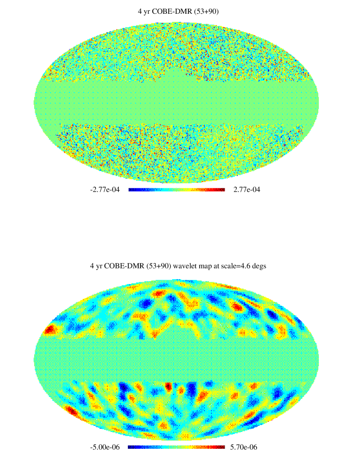
Figure 1: Analysed co-added COBE-DMR map (top) and the corresponding wavelet coefficient map obtained at $4.6$ degrees (bottom).

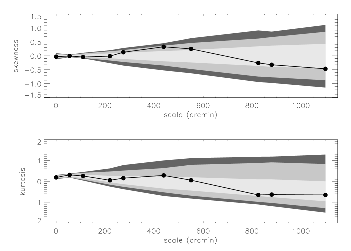
Figure 2: Skewness values obtained from the analysed co-added COBE-DMR map at several scales are represented by dots in the top figure. The bands represent the $68\%$, $95\%$ and $99\%$ confidence levels. The corresponding kurtosis results are presented in the bottom figure. Values at zero correspond to real space.

2 The Spherical Mexican Hat Wavelet

In many cases of astrophysical interest, data are given on the sphere. In this paper, we are interested in the analysis of the COBE-DMR data in the HEALPix pixelisation (Górski, Hivon & Wandelt 1999), but current and future experiments measuring CMB anisotropy can also be investigated using these methods. A conventional analysis technique is based on spherical harmonic decomposition of the temperature anisotropy for which local information is lost. On the other hand, wavelets -defined on the line/plane- have been extensively used (spectral and image analysis) in astrophysical applications during the last years. In particular, the continous isotropic wavelet transform of a 2D signal $f(\vec{x})$ is defined as

$$w(R,\vec{b})=\int d\vec{x}\,f(\vec{x})\Psi(R,\vec{b};\vec{x}),$$ (1)

being

$$\Psi(R,\vec{b};\vec{x})=\frac{1}{R}\psi(\frac{|\vec{x}-\vec{b}|}{R}),$$ (2)

and where $w(R,\vec{b})$ is the wavelet coefficient associated to the scale $R$ at the point with coordinates $\vec{b}$. The limits in the double integral are $-\infty$ and $\infty$ for the two variables. $\psi$ is the wavelet mother function that satisfies the constraints $\int d\vec{x}\,\psi=0,\int d\vec{x}\,{\psi}^{2}=1$, and the admissibility condition $C_{\psi}\equiv(2\pi)^{2}\int dk\,k^{-1}\,{\psi}^{2}(k)<\infty$, where $\psi(k),k\equiv|\vec{k}|$, is the Fourier transform of $\psi(x)$. A reconstruction of the image can be achieved with the inversion formula

$$f(\vec{x})=\frac{1}{C_{\psi}}\int dR\,d\vec{b}\frac{1}{R^{4}}w(R,\vec{b})\psi(\frac{|\vec{x}-\vec{b}|}{R}).$$ (3)

The analysis of 2D images can be done with the so-called Mexican Hat wavelet (MEXHAT). It is given by

$$\psi(x)=\frac{1}{{(2\pi)}^{1/2}}(2-x^{2})e^{-x^{2}/2},\ \ \ x\equiv|\vec{x}|,$$ (4)

that is proportional to the laplacian of a Gaussian. It has been sucessfully applied to extract point sources from CMB maps (Cayón et al. 2000, Vielva et al. 2000).

The problem arises when one tries to extend the continous isotropic wavelet to the sphere. There had been some proposals to do such an extension (e. g. analyzing functions defined through spherical harmonics, Freeden 1997; second generation wavelets, Sweldens 1996). However, one would like to incorporate the following properties: i) the transform is defined by a wavelet, i. e. $\int d\Omega{\Psi}_{S_{2}}=0$, ii) the wavelet transform must involve translations and dilations on the sphere and iii) for small scales the transform must reduce to the usual continous isotropic wavelet on the plane. Recently, Antoine & Vandergheynst (1998) have presented a group-theoretical derivation of the continous wavelet transform on the 2-sphere $S_{2}$ satisfyng the three previous conditions. They identify the appopriate transformations as: i) translations are given by elements of the 3D rotation group $SO(3)$; ii) dilations around any point are the inverse stereographic projection of standard dilations on the tangent plane to the point. Using polar coordinates $(\theta,\phi)$ around any fixed -but arbitrary- point on $S_{2}$, such a projection is defined by

$$x=2\tan\frac{\theta}{2},\ \ \ x\equiv|\vec{x}|,$$ (5)

where $(x,\phi)$ are polar coordinates on the tangent plane. Moreover, the analyzing wavelet, with respect to any fixed but arbitrary point, is given by (Martínez-González et al. 2001)

$${\Psi}_{S_{2}}(\theta;R)=N\frac{4}{{(1+\cos\theta)}^{2}}\psi(\frac{x}{R}=\frac{2}{R}\tan\frac{\theta}{2}),$$ (6)

where $N$ is a normalization constant given by

$$N={1\over R}{(1+\frac{R^{2}}{2}+\frac{R^{4}}{4})}^{-1/2},$$ (7)

being $\psi(x/R)$ the mother wavelet associated to the continous transform on the plane. $R$ defines the size of the Mexican Hat. Then, the generalization to $S_{2}$ of the MEXHAT on the plane is clearly given by eq. (6) with $\psi(x/R)$ given by eq. (4). Therefore, moving any point to the North Pole and taking polar coordinates, the wavelet coefficients associated to the function $f(\theta,\phi)$ are given at that point by

$$w(R)=\int d\Omega f(\theta,\phi){\Psi}_{S_{2}}(\theta;R).$$ (8)

3 Method

The methodology used in this work is designed to analyse the 4-year COBE-DMR data in the HEALPix pixelisation. Maps at 53 and 90 GHz are added using inverse-noise-variance weights. The resolution of these maps is $N_{side}=64$ corresponding to a pixel size of $\approx 55^{\prime}$ and resulting in 49152 pixels. Only those pixels surviving the extended Galactic cut of Banday et al. (1997) are considered (in order to excise those pixels with significant Galactic contamination near the plane of the Galaxy). Moreover, we subtract the best-fit monopole and dipole (as computed on the cut-sky) from the remaining pixels. We refer to the resulting map as the co-added COBE-DMR map.

The spherical Mexican Hat wavelet of several sizes is convolved with the co-added COBE-DMR map. The size of the Mexican Hat ($R$) fixes the characteristic scale of the wavelet coefficients (obtained after the convolution). Wavelet coefficient maps are obtained for several Mexican Hat sizes and statistical tests presented below are applied to these maps (see Figure 1 for an example of a wavelet coefficients map). Confidence intervals are estimated from simulations. We simulate CMB temperature fluctuations assuming a CDM power spectrum (computed using the CMBFAST software) with $\Omega_{b}=0.05$, $\Omega_{c}=0.3$, $\Omega_{v}=0.65$, $\Omega_{\nu}=0$, $H_{o}=65$ km/s/Mpc and $n=1$. The power spectrum is normalized to $Q_{rms-PS}=18\mu K$. Simulated maps are smoothed with a Gaussian beam of $FWHM=7.032^{\circ}$ (to approximate the beam response of the DMR instrument). Noise maps, generated with the same observation pattern and rms noise levels as the COBE-DMR data, are added to the simulated signal. The Galactic mask is also applied to the simulations, and the monopole and dipole components are estimated and subtracted outside the excluded region for each simulated map. Since the Mexican Hat wavelet extends to the whole sphere, convolution with the sky at a fixed pixel will involve information from pixels over all angular separations. However, in this analysis the wavelet coefficients must be computed excluding those pixels within the Galactic mask. In principle, this effect could bias the distribution we want to test. In practise, there is no appreciable change in results introduced by the partial sky coverage.

We have applied several tests in wavelet space that can be divided into two categories. The first ones are computed globally from wavelet coefficient maps at scales ranging from $55^{\prime}$ to $1760^{\prime}$. We have also computed these tests on the real map and results are indicated by scale $0^{\prime}$ in Figure 2 and Table 1. In addition we have also considered tests based on the derived distribution function at each pixel, at scales ranging from $108^{\prime}$ to $1728^{\prime}$. In this way we take into account the different amplitude of the noise at each pixel. The reason for considering scales different from the ones used in the previous case, is that the maximum resolution of the analysed COBE-DMR map and of the simulations is $N_{size}=32$ (corresponding to 12228 pixels on the sphere with size $1^{\circ}.8$). Information on temperature distributions at each pixel has to be kept at each scale. We needed to degrade the resolution to be able to handle all this information.

In the first category of tests we calculated different statistics commonly used to detect non-Gaussianity. Skewness and kurtosis will test the third ($\kappa_{3}$) and fourth ($\kappa_{4}$) order cumulants :

$$S=\kappa_{3}/\kappa_{2}^{3/2}\ \ \ K=\kappa_{4}/\kappa_{2}^{2}-3,$$ (9)

Correlations between two consecutive scales $k,j$ are tested using the conventional 2-scale correlation given by:

$$C_{2,1}(k,j)={{\sum_{i=1}^{N_{p}}\Delta T/T(k,i)\Delta T/T(j,i)}\over{N_{p}V(k)V(j)}}$$ (10)

where

$$V(k)=({{\sum_{i=1}^{N_{p}}(\Delta T/T(k,i))^{2}}\over{N_{p}}})^{1/2}$$ (11)

and $N_{p}$ will correspond to the number of pixels considered at the largest scale (the ones outside the Galactic mask located at a distance from the border larger than twice the Mexican Hat size corresponding to that scale). As well as a correlation analogous to the one used by Barreiro et al. 2000, given by:

$$C_{2,2}(k,j)={{\sum_{i=1}^{N_{p}}(\Delta T/T(k,i))^{2}(\Delta T/T(j,i))^{2}}\over{V(k)V(j)}}$$ (12)

We have also considered correlations between three consecutive scales $k,j,l$ given by:

$$C_{3}(k,j,l)={{\sum_{i=1}^{N_{p}}\Delta T/T(k,i)\Delta T/T(j,i)\Delta T/T(l,i)}\over{N_{p}V(k)V(j)V(l)}}$$ (13)

In addition we compare the temperature fluctuation distributions from the data to those obtained from simulations, at several scales. The Kolmogorov-Smirnov test is used in this comparison. We have calculated the distance parameter for the COBE-DMR data as well as a distance parameter distribution from simulations.

In the second category of tests we have calculated wavelet coefficient distributions at each pixel at each scale. We compute the probability of extrema taking into account the dispersion at each pixel. The second of these tests consists in the following. At a fixed scale, for the COBE-DMR data we select those pixels with values outside the $99\%$ and $95\%$. The number of those selected pixels is compared with the expected number from simulations.

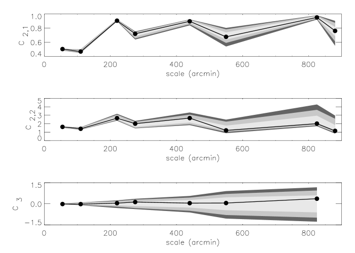
Figure 3: Values corresponding to the 2-scale correlation $C_{2,1}$ are presented in the top figure. At each scale, the correlation has been calculated with the scale directly above (i.e. the value at $55^{\prime}$ corresponds to the correlation between wavelet coefficients at $55^{\prime}$ and $110^{\prime}$). The scales are the same ones appearing in Table 1, from $55^{\prime}$ to $1100^{\prime}$. Bands correspond to confidence levels at $68\%$, $95\%$ and $99\%$. The middle figure presents the results for the 2-scale correlation defined as in Barreiro et al. 2000 $C_{2,2}$. The figure in the bottom corresponds to the correlation between three consecutive scales. At each scale the value presented is the correlation between that scale and the other two direclty above that one (i.e. at $55^{\prime}$ the correlation is calculated between wavelet coefficients at that scale and $110^{\prime}$ and $220^{\prime}$).

Table 1: Kolmogorov-Smirnov distance dKS

scale(’)	dKS(COBE)	Max dKS
0	0.028	0.035
55	0.036	0.043
110	0.034	0.041
220	0.033	0.052
275	0.029	0.068
440	0.036	0.137
550	0.030	0.173
825	0.088	0.296
880	0.107	0.351
1100	0.220	0.560

Table 2: Probability of Extrema

scale (’)	Prob($T$$\geq$ $T_{max}COBE$) $\%$	Prob($T\leq T_{min}COBE$)$\%$	Prob($|(T/\sigma_{pix})|\geq|(T/\sigma_{pix})_{max}COBE|$)$\%$
108	84.2	80.6	96.8
324	38.4	86.6	82.6
432	15.4	90.6	41.6
648	24.0	84.4	44.6
864	67.6	62.4	78.2

Table 3: Probability of Areas outside the $99\%$ and the $95\%$

scale (’)	COBE pix out $99\%$	Prob(pix out $99\%\geq$ COBE) $\%$	COBE pix out $95\%$	Prob(pix out $95\%\geq$ COBE) $\%$
108	87	0.0	359	2.0
324	44	37.0	187	82.4
432	34	48.4	161	77.6
648	18	45.6	50	89.2
864	0	100.0	22	82.0

4 Results and Conclusions

We have applied the statistical tests described in the previous section to the COBE-DMR data. 500 Gaussian simulations were performed to obtain the confidence intervals for each test as well as the distribution functions at each pixel. The results are summarised in figures 2 and 3 and tables 1, 2 and 3. For the tests in the first category, corresponding to figures 2 and 3, all but one of the COBE-DMR values are inside the $95\%$ confidence interval. In the case of $C_{2,1}$ between scales $55^{\prime}$ and $110^{\prime}$, the value for the COBE-DMR is inside the $99\%$ confidence interval. Since the correlations are calculated between scales that do not differ from each other by a constant amount, one can observe an oscillating behaviour for $C_{2,1}$ and $C_{2,2}$. Some peaks occur when the correlation is calculated between two scales differing by a small amount. Also part of the first category tests, the Kolmogorov-Smirnov distance obtained from the COBE-DMR data is, at all scales, smaller than the maximum found for the 500 Gaussian simulations (Table 1). In the second category of tests (Tables 2 and 3), only the probability of finding a number of pixels outside the $99\%,95\%$ confidence intervals, greater or equal the number of COBE-DMR pixels found outside those intervals, at the smallest scale ($108^{\prime}$), is very low. However, noise might be dominating at this scale. Therefore, no obvious deviation from Gaussianity can be noted from any of the tests presented in this work.

The spherical Mexican Hat wavelet is introduced in this paper as a tool to study the information at different scales in the COBE-DMR data. The only other wavelet on the sphere previously used to analyse CMB data is the spherical Haar wavelet (Tenorio et al. 1999, Barreiro et al. 2000). The main difference between these two wavelets is the geometrical property of isotropy that characterises the Mexican Hat. The Haar wavelet however biases certain directions. As a consequence, orientation of the data has to be taken into account in case this last wavelet is used in the analysis. The formalism of projecting the Mexican Hat (defined on the plane) on the surface of the sphere was presented in Section 2. Specific details related for example to the implementation on the HEALPix pixelitation will be given in Martínez-González et al. (2001).

In summary, several statistical tests have been performed in wavelet space. They are divided in two categories. The first one includes tests performed globally on the wavelet coefficient maps. Tests in the second category take into account local properties at each scale. Temperature fluctuation distributions are computed from Gaussian simulations at each pixel at each scale. The local dispersion is considered in the statistical tests applied. These methods have not been applied in any of the previous works. From all of them we can conclude that the analysed COBE-DMR data are compatible with Gaussianity. Skewness, kurtosis and $C_{2,2}$ were also tested by Barreiro et al. 2000 with the spherical Haar wavelet. There is no indication from this work that one of the two wavelets is more optimal for detecting non-Gaussian features in the COBE-DMR data. However, the Mexican Hat wavelet is more localized in wavelet space than the Haar wavelet. Moreover, a comparison of the performance on the sphere of the two wavelets shows, that the spherical Mexican Hat wavelet is more optimal than the spherical Haar wavelet for detecting certain non-Gaussian features (Martínez-González et al. 2001).

References

- [1] Aghanim, N., Forni, O. & Bouchet, F.R. 2000, astro-ph/0009463
- [2] Antoine, J.-P. & Vandergheynst, P., 1998, J. of Math. Phys., 39, 3987
- [3] Banday, A.J., Górski, K.M., Bennett, C.L., Hinshaw, G., Kogut, A., Lineweaver, C.H., Smoot, G.F., & Tenorio, L. 1997, ApJ, 475, 393
- [4] Banday, A.J., Zaroubi, S. & Górski, K.M. 2000, ApJ, 533, 575
- [5] Barreiro, R.B., Sanz, J.L., Martínez-González, E., Cayón, L. & Silk, J. 1997, ApJ, 478, 1
- [6] Barreiro, R.B., Sanz, J.L., Martínez-González, E. & Silk, J. 1998, MNRAS, 296, 693.
- [7] Barreiro, R.B., Martínez-González, E. & Sanz, J.L. 1999, astro-ph/0009365
- [8] Barreiro, R.B., Hobson, M.P., Lasenby, A.N, Banday, A.J., Górski, K.M. & Hinshaw, G. 2000, MNRAS, 318, 475
- [9] Bond, J.R. & Efstathiou, G. 1987, MNRAS, 226, 655
- [10] Cayón, L., Sanz, J. L., Barreiro, R. B., Vielva, P., Toffolatti, L., Silk, J., Diego, J. M. & Argueso, F., 2000, MNRAS, 315, 757
- [11] Diego, J.M., Martínez-González, E., Sanz, J.L., Mollerach, S. & Martínez, V.J. 1999, MNRAS, 306, 427
- [12] Ferreira, P.J., Magueijo, J. & Górski, K. 1998, ApJ, 503, L1
- [13] Freeden, W., Schreiner, M. & Gervens, T., 1997, ”Constructive Approximation on the sphere, with applications to Geomathematics”, Clarendon Press, Oxford
- [14] Górski, K.M., Hivon, E. & Wandelt, B.D. (astro-ph/9812350) 1999, Proceedings of the MPA/ESO Conference on Evolution of Large-Scale Structure: from Recombination to Garching, 2-7 August 1998; eds. A.J. Banday, R.K. Sheth and L. Da Costa, PrintPartners IPSKAMP NL (1999)
- [15] Gott III, J.R., Park, C., Juszkiewicz, R., Bies, W.E., Bennett, D.P., Bouchet, F.R. & Stebbins, A. 1990, ApJ, 352, 1
- [16] Heavens, A.F. 1998, MNRAS, 299, 805
- [17] Hobson, M.P., Jones, A.W. & Lasenby, A.N. 1999, MNRAS, 309, 125
- [18] Kogut, A., Banday, A.J., Bennett, C.L., Górski, K., Hinshaw, G., Smoot, G.F. & Wright, E.L. 1996, ApJ, 464, L29
- [19] Luo, X. & Schramm, D.N. 1993a, ApJ, 408, 33
- [20] Luo, X. & Schramm, D.N. 1993b, PRL, 71, 1124
- [21] Luo, X. 1994, ApJ, 427, L71
- [22] Magueijo, J. 2000, ApJ, 528, L57
- [23] Martínez-González, E. & Sanz, J.L. 1989, MNRAS, 237, 939
- [24] Martínez-González, E. et al. 2001, in preparation
- [25] Mollerach, S., Martínez, V.J., Diego, J.M., Martínez-González, E., Sanz, J.L. & Paredes, S. 1999, ApJ, 525, 17
- [26] Mukherjee, P., Hobson, M.P. & Lasenby, A.N. 2000, MNRAS, 318, 1157
- [27] Netterfield, C.B. et al. 2001, astro-ph/0104460
- [28] Novikov, D., Schmalzing, J. & Mukhanov, V.F. 2000, astro-ph 0006097
- [29] Pando, J. Valls-Gabaud, D., Fang, L.Z. 1998, Phys.Rev.Lett., 81, 4568
- [30] Pompilio, M.P., Bouchet, F.R., Murante, G. & Provenzale, A. 1995, ApJ, 449, 1
- [31] Pryke, C. et al. 2001, astro-ph/0104490
- [32] Schmalzing, J. & Górski, K.M. 1997, MNRAS, 297, 355
- [33] Stompor, R. et al. 2001, astro-ph/0105062
- [34] Sweldens, W., 1996, Applied Comput. Harm. Anal., 3, 1186
- [35] Tenorio, L., Jaffe, A.H., Hanany, S. & Lineweaver, C.H. 1999, MNRAS, 310, 823
- [36] Torres, S., Cayón, L., Martínez-González, E. & Sanz, J.L. 1995, MNRAS, 274, 853
- [37] Vielva, P., Barreiro, R. B., Hobson, M. P., Martínez-González, E., Lasenby, A. N., Sanz, J. L. & Toffolatti, L., 2000, submitted
- [38] Vittorio, N. & Juszkiewicz, R. 1987, ApJ, 314, L29
- [39] White, R.A & Stemwedel, S.W. 1992, in ADASS I, ed. Worrall, D.M., Biemesderfer, C., & Barnes, J., San Francisco, ASP, pp 379