Numerical Simulation of Non-Gaussian Random Fields
with Prescribed Correlation Structure

Abstract

In this paper we will consider the problem of the numerical simulation of non-Gaussian, scalar random fields with a prescribed correlation structure provided either by a theoretical model or computed on a set of observational data. Although, the numerical generation of a generic, non-Gaussian random field is a trivial operation, the task becomes tough when constraining the field with a prefixed correlation structure. At this regards, three numerical methods, useful for astronomical applications, are presented. The limits and capabilities of each method are discussed and the pseudo-codes describing the numerical implementation are provided for two of them.

1 INTRODUCTION

Computer-aided modeling is becoming an essential tool in designing new experiments and in testing theoretical models against the observational data. For example, because of the cost of any space-based telescope, nowadays it is not even conceivable to plan a mission without first simulating the performances either of the instruments and/or of the observing mode. It is obvious to stress that the reliability of such simulations depends critically on the possibility to reproduce realistic physical scenarios.

A wide assumption, which is often made because of its simplicity, is that the processes underlying a given physical phenomenon obey Gaussian, and therefore linear, statistics. However, although as practical as this assumption could be, it is not applicable for most of the physical systems which, on the contrary, are expected to be characterized by nonlinear behaviours. Some examples:

• the high spatial resolution observations of sky images are revealing a lot of details of the sky emission which are not of easy interpretation (e.g. Herbstmeier et al. (1998)). For istance, in the far infrared spectral domain, the studies of source properties imply the disentangling of the source emission and position from those of a much stronger background whose spatial structure is highly non-Gaussian. This task becomes crucial for most space-borne surveys of the extragalactic sky and of star-forming regions in the Galaxy for which it is of interest to simulate the far-IR and sub-mm emission of the Galaxy and the source confusion in the beam. Their nature is intrinsically non-Gaussian and to match their observed properties an appropriate method must be used.

• The interpretation of the new flow of data on the Cosmic Microwave Background (CMB) spatial distribution, from present and future experiments (BOOMERANG, MAXIMA, MAP and PLANCK), is involving a large theoretical effort (see e.g. Verde et al. (2000); Matarrese, Verde & Jimenez (2000); Contaldi & Magueijo (2001) and references therein). Studies of the spatial structure of the CMB provide fundamental clue on the physical processes generating the primordial density fluctuations which are thought to be at the origin of the present-day structures. There are deep theoretical motivations, both in the framework of inflationary models and in cosmological defects scenarios, to consider the initial density perturbations obeying non-Gaussian statistics. In any case, the subsequent growth of these density fluctuations, triggered by the gravitational potential, makes the late time evolution nonlinear. The testing of these predictions requires algorithms able to discerne the true statistical nature of the observed fields. Some of their properties can be analytically recovered but the bulk of non-Gaussian random fields characteristics can be inferred only through simulations (see e.g., Moscardini et al. (1991)).

The aim of this paper is to provide a general and mathematical approach to the problem of generating non-Gaussian random fields when a correlation structure is given either by a theoretical model or by the statistical analysis of experimental data. Some numerical procedures to perform simulations of such fields are also presented. The arguments are outlined on a quite general basis in view of applications in a wide astrophysical context. The reason to fix the correlation structure is that this is the simplest way to obtain non-trivial (i.e. non-pure noise) fields (see below).

The problem can be formalized as follows. A real, random field $R({\bf t})$ can be defined as a collection of random variables $\{{\bf r}\}$ at points with coordinates $\{{\bf t}\}=\{(t_{1},t_{2},\ldots,t_{n})\}$ in a n-th dimensional “parameter space”. In other words, for each “position” $\hat{\bf t}$, $R(\hat{\bf t})={\bf r}$, where ${\bf r}$ is a vector characterized by a multidimensional distribution function $F_{R}({\bf r})$ and a multidimensional probability density function $f_{R}({\bf r})$. According to the particular problem at hand, $\{{\bf t}\}$ may correspond to a set of spatial/angular coordinates (spatial random fields), to time (time processes), to a mix of these two (spatio-temporal random fields) or even to more general situations.

In many practical situations they are of interest the so called scalar random fields, where ${\bf r}\equiv r$. This means that for a specific $\hat{\bf t}$, $R(\hat{\bf t})$ is characterized by a scalar random variable $r$ with one-dimensional distribution function (DF) $F_{R}(r)$ and one-dimensional probability density function (PDF) $f_{R}(r)$. In this paper we will consider only this kind of random fields. The more general case of vector-valued random fields represents a more complex problem and will not be addressed in this work (for more details about this topic see Popescu, Deodatis & Prevost (1998)).

The main problem in the numerical simulation of a generic $R({\bf t})$ is that, in general, given two arbitrary “positions”, say ${\bf t}_{1}$ and ${\bf t}_{2}$, $R({\bf t}_{1})$ and $R({\bf t}_{2})$ are not independent one of the other. As well known from the standard theory of random processes (e.g. Grigoriu (1995)), the practical applications to generate random fields requires to put some constraints. The most common choice is that, specified the distribution function $F_{R}(r)$, $R({\bf t})$ be completely characterized by the covariance function, $\xi_{R}({\bf t}_{1},{\bf t}_{2})$, with

$$\xi_{R}({\bf t}_{1},{\bf t}_{2})={\rm E}\left[R({\bf t}_{1})~{}R({\bf t}_{2})\right],$$ (1)

where ${\rm E}[.]$ stands for expected value. The reason is that $\xi_{R}({\bf t}_{1},{\bf t}_{2})$ represents the simplest form of mutual relationship between the elements of $R({\bf t})$.

In astronomical applications, very often it is possible to adopt some simplifying conditions. In particular, it is possible to assume that $R({\bf t})$ is isotropic. This means that the covariance function depends on the length of the vector ${\bf t}_{1}-{\bf t}_{2}$ but not on its direction: $\xi_{R}({\bf t}_{1},{\bf t}_{2})=\xi_{R}(\|{\bf t}_{1}-{\bf t}_{2}\|)$ . In other words, $R({\bf t})$ is characterized by a spherical symmetry. This property is very useful since it allows to characterize $R({\bf t})$ through the correlation function

$$\rho_{R}(\tau)={\rm E}\left[\frac{(R({\bf t})-\mu_{R})~{}(R({\bf t}+{\mbox{\boldmath$\tau$}})-\mu_{R})}{\sigma_{R}^{2}}\right],$$ (2)

where $\tau=\|{\mbox{\boldmath$\tau$}}\|$, and $\mu_{R}$ and $\sigma^{2}_{R}$ are, respectively, the mean and the variance corresponding to the distribution $F_{R}(r)$.

Although the isotropic case is of large interest in astronomical applications, here we prefer to adopt a more general formalism, suited for all homogeneous fields. Indeed, in this case, the covariance function depends on ${\bf t}_{1}-{\bf t}_{2}$. According to this definition, $\rho(\tau)$, in equation (2) has to be replaced by $\rho({\mbox{\boldmath$\tau$}})$.

2 PRELIMINARY NOTES

Most of the techniques for simulating a non-Gaussian, scalar, random field $R({\bf t})$, with a prescribed correlation function, $\rho_{R}({\mbox{\boldmath$\tau$}})$, and a prescribed one-dimensional marginal $F_{R}(r)$, are more or less explicitly based on the two following steps:

• generation of a zero-mean, unit-variance, scalar, Gaussian random field $X({\bf t})$ with a prefixed correlation structure $\rho_{X}({\mbox{\boldmath$\tau$}})$;

• mapping (transformation) $X({\bf t})\rightarrow R({\bf t})$ according to

  $$R({\bf t})=g[X({\bf t})],$$ (3)

  where $g[.]$ represents an appropriate function. This operation is named memoryless transformation since the value of $R({\bf t})$ at an arbitrary $\hat{\bf t}$ depends only on the value of $X(\hat{\bf t})$.

The rationale behind such a procedure is that the direct generation of a generic $R({\bf t})$, with a specific $\rho_{r}({\mbox{\boldmath$\tau$}})$, is a very difficult operation. The Gaussian case represents a useful exception. Hence, it results much easier to obtain $R({\bf t})$ by transforming a precomputed $X({\bf t})$. However, after the mapping (3), in general $\rho_{X}({\mbox{\boldmath$\tau$}})$ does not coincide with $\rho_{R}({\mbox{\boldmath$\tau$}})$. Therefore, it is necessary to transform an $X({\bf t})$ characterized by an appropriate $\rho_{X}({\mbox{\boldmath$\tau$}})$ whose functional form depends on $\rho_{R}({\mbox{\boldmath$\tau$}})$.

It is well known from elementary statistics that for a mapping $r=g(x)$, with $x$ the standard one-dimensional Gaussian variable, the PDF of the random variable $r$ can be obtained from that of the random variable $x$ via a change of variable technique. In the general case that the tranformation $g(.)$ is not one-to-one, if the equation

$$g(x)-r=0$$ (4)

has a numerable set of $M$ real solutions $\{x_{1}(r),x_{2}(r),\ldots,x_{M}(r)\}$, and if $g_{j}^{\prime}=[dg(x)/dx]_{x=x_{j}}$, $j=1,2,\ldots,M$ exist, then $f_{R}(r)$ is given by (Papoulis, 1991)

$$f_{R}(r)=\frac{1}{\sqrt{2\pi}}\sum_{j=1}^{M}\frac{{\rm e}^{-x_{j}^{2}(r)/2}}{\left|g_{j}^{\prime}\right|}.$$ (5)

In correspondence to the values $r^{*}$, where equation (4) does not have real solutions, it happens that $f_{R}(r^{*})=0$. Furthermore, the correlation function $\rho_{R}({\mbox{\boldmath$\tau$}})$ is given by (Grigoriu, 1995)

$$\rho_{R}({\mbox{\boldmath$\tau$}})=\frac{1}{\sigma_{R}^{2}}\int_{-\infty}^{\infty}\int_{-\infty}^{\infty}[g(x_{1})-\mu_{R}]~{}[g(x_{2})-\mu_{R}]~{}\phi(x_{1},x_{2};\rho_{X}({\mbox{\boldmath$\tau$}}))~{}dx_{1}~{}dx_{2},$$ (6)

where, $x_{1}=x({\bf t})$ and $x_{2}=x({\bf t}+{\mbox{\boldmath$\tau$}})$, and

$$\phi(x_{1},x_{2};\rho_{X}({\mbox{\boldmath$\tau$}}))=\frac{1}{2\pi(1-\rho_{X}^{2}({\mbox{\boldmath$\tau$}}))^{1/2}}~{}\exp\left(-\frac{x_{1}^{2}+x_{2}^{2}-2\rho_{X}({\mbox{\boldmath$\tau$}})x_{1}x_{2}}{2(1-\rho_{X}^{2}({\mbox{\boldmath$\tau$}}))}\right).$$ (7)

At first sight, from these equations it may seem that, given the appropriate function $g(.)$ and the covariance function $\rho_{X}({\mbox{\boldmath$\tau$}})$, obtained via the inversion of equation (6), it is possible to generate an $R({\bf t})$ characterized by an arbitrary $\rho_{R}({\mbox{\boldmath$\tau$}})$. In reality, given a generic $g(.)$, there is no guarantee that equation (6) can be inverted. Furthermore, it is possible to show (Ogorodnikov & Prigarin, 1996) that $\rho_{R}({\mbox{\boldmath$\tau$}})$ can take values only in the interval

$$\rho_{R}({\mbox{\boldmath$\tau$}})\in[\rho^{*},1],$$ (8)

where

$$\rho^{*}=\frac{1}{\sigma_{R}^{2}}\left(\int_{0}^{1}F_{R}^{-1}(\alpha)~{}F_{R}^{-1}(1-\alpha)~{}d\alpha-\mu_{R}^{2}\right),$$ (9)

with

$$F_{R}^{-1}(\alpha)=\inf\{r:F_{R}(r)>\alpha\}$$ (10)

providing the smallest value of the random variable $r$ satisfying the condition that $F_{R}(r)>\alpha$. In particular, $\rho^{*}=-1$ only for symmetric distributions. For example, $\rho^{*}\simeq-0.645$ in case of the exponential PDF: $f_{R}(r)=\beta~{}\exp(-\beta r),r\geq 0$. This shows that, in general, for a fixed $g(.)$ it is not possible to obtain a $\rho_{R}^{*}({\mbox{\boldmath$\tau$}})$ presenting values external to the interval (8).

Another problem stems from the fact that the function $\rho_{X}({\mbox{\boldmath$\tau$}})$, necessary to obtain the target $\rho_{R}({\mbox{\boldmath$\tau$}})$ via equation (6), must be a non-negative definite function otherwise the generation of the aimed $R({\bf t})$ is prevented since $\rho_{X}({\mbox{\boldmath$\tau$}})$ does not represent any correlation function.

In principle, equation (6) can be used to obtain $\rho_{X}({\mbox{\boldmath$\tau$}})$ in a closed form, but in reality such an approach can be followed only in a limited number of cases. Indeed, very often the transformation (6) has a very complex form and can be inverted only via a numerical approach.

3 ANALYTICAL METHOD

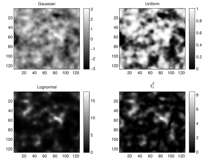
Figure 1: Examples of non-Gaussian random fields characterized by the same correlation function.

Certainly one of the most effective method for generating $R({\bf t})$ is represented the analytical handling of equations (5) and (6). Unfortunately, this is also the most difficult approach to pursue; only in a limited number of cases it has been possible to find out the analytical relationship between $\rho_{X}({\mbox{\boldmath$\tau$}})$ and $\rho_{R}({\mbox{\boldmath$\tau$}})$. Some useful examples are presented below (see also figure 1):

3.1 Lognormal Fields

If $X({\bf t})$ is a homogeneous, zero-mean, unit-variance Gaussian fields with a correlation function $\rho_{X}({\mbox{\boldmath$\tau$}})$, the random fields obtained via

$$L({\bf t})=e^{\mu+\sigma X({\bf t})}$$ (11)

are called Lognormal fields since they are characterized by the one-dimensional marginal Lognormal PDF

$$f_{L}(l)=\frac{1}{l~{}\sigma\sqrt{2\pi}}~{}e^{-\left(\ln l-\mu\right)^{2}/(2\sigma^{2})},\qquad l>0.$$ (12)

It is possible to show (Vanmarke, 1984) that the moments of order $k$ of $L({\bf t})$ are given by

$$E[L^{k}]=e^{k\mu+k^{2}\sigma^{2}/2}.$$ (13)

In particular, the mean and the variance are

$$\mu_{L}=e^{\mu+\sigma^{2}/2},\qquad\sigma^{2}_{L}=e^{2\mu+\sigma^{2}}(e^{\sigma^{2}}-1),$$ (14)

respectively. Furthermore, it is possible to show that the relationship between $\rho_{L}({\mbox{\boldmath$\tau$}})$ and $\rho_{X}({\mbox{\boldmath$\tau$}})$ can be expressed in the form

$$\rho_{L}({\mbox{\boldmath$\tau$}})=\frac{e^{\sigma^{2}\rho_{X}({\mbox{\boldmath$\tau$}})}-1}{e^{\sigma^{2}}-1}.$$ (15)

From this equation it is trivial to see that, when $\sigma=1$, the lower bound of $\rho_{L}({\mbox{\boldmath$\tau$}})$ is $\simeq-0.368$.

3.2 Gamma Fields

If $X_{s}({\bf t})$, $s=1,2,\ldots,2m$, is a collection of independent zero-mean, unit-variance Gaussian fields with the same correlation function $\rho_{X}({\mbox{\boldmath$\tau$}})$, the random fields obtained via

$$G_{m}({\bf t})=\frac{1}{2}\sum_{s=1}^{2m}X_{s}^{2}({\bf t})$$ (16)

are called Gamma fields. That is because the corresponding one-dimensional marginal PDF is a Gamma distribution with $m$ degrees of freedom

$$f_{G_{m}}(g)=\frac{1}{\Gamma(m)}~{}g^{m-1}e^{-g},\qquad g\geq 0,$$ (17)

where $\Gamma(.)$ is the Gamma function.

It can be shown that the moments of order $k$ of $G_{m}$ are given by

$$E[G_{m}^{k}]=\frac{\Gamma(m+k)}{\Gamma(m)}=\prod_{i=0}^{k-1}(m+i),\qquad k>-m.$$ (18)

In particular, the mean and the variance are

$$\mu_{G_{m}}=\sigma^{2}_{G_{m}}=m.$$ (19)

It can also be shown (Hasofer, Ditlevsen & Tarp-Johansen, 1998) that, idependently from the value of $m$, the relationship between $\rho_{G_{m}}({\mbox{\boldmath$\tau$}})$ and $\rho_{X}({\mbox{\boldmath$\tau$}})$ can be expressed in the form

$$\rho_{G_{m}}({\mbox{\boldmath$\tau$}})=\rho_{X}^{2}({\mbox{\boldmath$\tau$}}).$$ (20)

The class of the Gamma fields is interesting since it contains, as particular cases, both the Chi-Square and the Exponential fields.

From equation (20) it appears that the lower bound of $\rho_{G_{m}}({\mbox{\boldmath$\tau$}})$ is zero. In other words, through the mapping (16) it is not possible to obtain $G_{m}({\bf t})$ characterized by correlation functions with negative values. Here, however, it is necessary to stress that such a limit is not intrinsic to the Gamma fields, but only to the transformation (16). In fact, through different mappings it is possible to generate $G_{m}({\bf t})$ with correlation functions having negative values (see below).

3.3 Beta Fields

Given two independent Gamma fields, say $G_{m}({\bf t})$ and $G_{n}({\bf t})$, characterized by the same correlation function $\rho_{G}({\mbox{\boldmath$\tau$}})$, the random fields obtained via

$$B_{mn}({\bf t})=\frac{G_{m}({\bf t})}{G_{m}({\bf t})+G_{n}({\bf t})}$$ (21)

are called Beta fields because their one-dimensional marginal PDF is a Beta$(m,n)$ distribution

$$f_{B_{mn}}(b)=\frac{1}{B(m,n)}~{}x^{m-1}(1-x)^{n-1},\qquad 0\leq b\leq 1.$$ (22)

It can be shown that the moments of order $k$ of $B_{mn}$ are given by

$$E[B^{k}]=\frac{\Gamma(m+k)\Gamma(m+n)}{\Gamma(m)\Gamma(m+n+k)}.$$ (23)

In particular, the mean and the variance are

$$\mu_{B_{mn}}=\frac{m}{m+n},\qquad\sigma^{2}_{B_{mn}}=\frac{mn}{(m+n)^{2}(m+n+1)},$$ (24)

respectively.

It can be also shown (Hasofer, Ditlevsen & Tarp-Johansen, 1998) that the relationship between $\rho_{B_{mn}}({\mbox{\boldmath$\tau$}})$ and $\rho_{X}({\mbox{\boldmath$\tau$}})$ can be expressed in the form

$$\rho_{B_{mn}}({\mbox{\boldmath$\tau$}})=1-S_{m+n}[\rho_{X}({\mbox{\boldmath$\tau$}})],\qquad n+m>1,$$ (25)

where

$$S_{q}(\rho)=q\left(\frac{1-\rho}{-\rho}\right)^{q}\left[\log(1-\rho)-\sum_{i=1}^{q-1}\frac{1}{i}\left(\frac{-\rho}{1-\rho}\right)^{i}\right],\qquad 0\leq\rho\leq 1,~{}q\in\{1,2,\ldots\},$$ (26)

with the end values $S_{q}(0)=1$ and $S_{q}(1)=0$. The class of the Beta fields is basic for describing variables bounded at both sides. For example, $B_{11}({\bf t})$ corresponds to the Uniform field.

As well as for the Gamma fields, also for the Beta fields obtained through mapping (21) it happens that the lower bound of $\rho_{B_{mn}}({\mbox{\boldmath$\tau$}})$ is zero. Again, this limit is not intrinsic to the Beta fields but only to the particular mapping used.

4 NUMERICAL METHOD

In case one is interested in a $R({\bf t})$ characterized by an $F_{R}(r)$ not reproducible through a function $g(.)$ available in analytical form and/or that does not permit an easy calculation of $\rho_{X}({\mbox{\boldmath$\tau$}})$, it is necessary to resort to numerical methods. Regarding this, the following presents three methods that can be useful in astronomical applications.

4.1 Change of Variable Method

The most obvious method is based on the numerical inversion of equation (6). Whenever possible, this is the ’method’ to use since, contrary to the procedures presented below, it is able to provide exact results (within the limits of the numerical computation). In particular, this inversion operation is feasible when $g(.)$ is a monotonic increasing, real function. Indeed, in this case the relationship between $\rho_{R}({\mbox{\boldmath$\tau$}})$ and $\rho_{X}({\mbox{\boldmath$\tau$}})$ can always be inverted.

In the case of distributions $F_{r}$ with no atoms (a concentration of a finite probability mass at a point), a very useful kind of monotonic increasing functions $g(.)$ is represented by the mapping

$$R({\bf t})=F^{-1}_{R}\{F_{X}[X({\bf t})]\},$$ (27)

where $F_{X}$ denotes the Gaussian distribution function and $F^{-1}_{R}$ the inverse distribution function of $R({\bf t})$. Indeed, through $g(.)=F^{-1}_{R}\{F_{X}(.)\}$ the generation of fields $R({\bf t})$, with arbitrary one-dimensional marginal distribution functions, is possible. Furthermore, it can be shown (Ogorodnikov & Prigarin, 1996; Grigoriu, 1995) that via the mapping (27) it is possible to obtain $R({\bf t})$ characterized by $\rho_{R}({\mbox{\boldmath$\tau$}})$ fully exploiting the interval (8) with $\rho^{*}$ that can be simplified to the form

$$\rho^{*}=\frac{{\rm E}[g(x)~{}g(-x)]-\mu_{R}^{2}}{\sigma_{R}^{2}}.$$ (28)

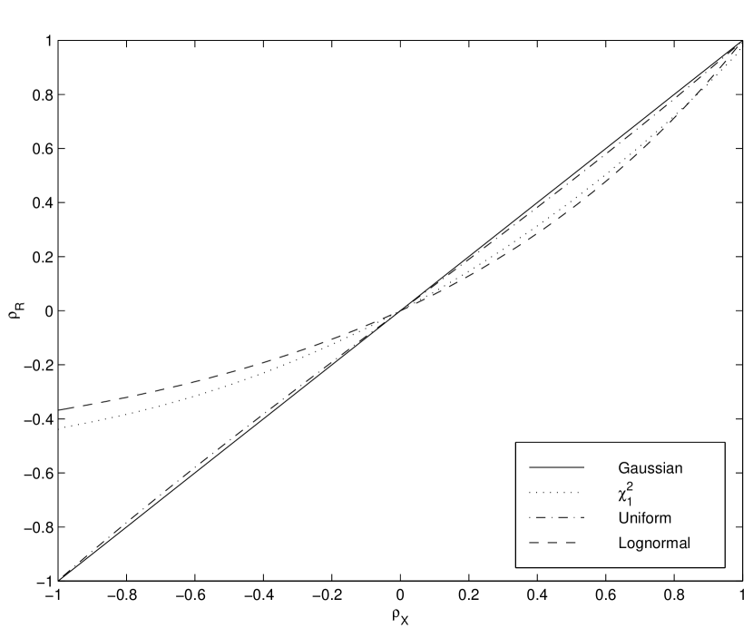
Figure 2: Relationship between the correlation function $\rho_{R}(\tau)$ of some non-Gaussian random fields obtained via transformation (27) and the correlation function $\rho_{X}(\tau)$ of the Gaussian fields used in such transformation.

Figure 2 shows the relationship between $\rho_{X}$ and the $\rho_{R}$, concerning some well known $F_{R}$, obtained via equations (27) and (6). From this figure it is possible to realize some interesting points that can also be proved via theoretical arguments (Grigoriu, 1995, 1998):

• $\rho_{R}({\mbox{\boldmath$\tau$}})$ is an increasing function of $\rho_{X}({\mbox{\boldmath$\tau$}})$;

• $|\rho_{R}({\mbox{\boldmath$\tau$}})|\leq|\rho_{X}({\mbox{\boldmath$\tau$}})|$;

• the difference between $\rho_{R}({\mbox{\boldmath$\tau$}})$ and $\rho_{X}({\mbox{\boldmath$\tau$}})$ are not significant for a broad range of values of these functions.

As explained in Section 2, once $\rho_{X}({\mbox{\boldmath$\tau$}})$ has been calculated, it is necessary to check that this function is non-negative definite. A possibility consists in evaluating the Fourier transform of $\rho_{X}({\mbox{\boldmath$\tau$}})$ and verifying that it presents no negative values.

The only concern regarding the numerical inversion of equation (6) is that, in general, this operation requires the calculation of a large number of double integrals. In certain situations, that could represent a computationally too expensive problem, and therefore it is necessary to resort to other numerical techniques.

4.2 Hermite Expansion Method

An alternative approach for the simulation of a non-Gaussian $R({\bf t})$ is based on the expansion of the field in Hermite polynomials. These polynomials can be defined through the Rodriguez’s formula

$${\rm H}_{n}(x)=(-1)^{n}e^{x^{2}/2}\frac{d^{n}}{dx^{n}}e^{-x^{2}/2},\qquad n=0,1,\ldots,$$ (29)

and have the important property of being orthogonal relative to the standard Gaussian distribution, so that

$$\int_{-\infty}^{+\infty}{\rm H}_{m}(x){\rm H}_{n}(x)~{}\frac{1}{\sqrt{2\pi}}~{}e^{-x^{2}/2}dx=n!~{}\delta_{mn}$$ (30)

where $\delta_{mn}$ is the Kronecker function.

An explicit expression for ${\rm H}_{n}(x)$ is given by Blinnikov & Moessner (1998)

$${\rm H}_{n}(x)=n!\sum_{k=0}^{\lfloor n/2\rfloor}\frac{(-1)^{k}x^{n-2k}}{k!(n-2k)!~{}2^{k}},$$ (31)

where $\lfloor z\rfloor$ means the largest integer $k\leq z$.

A field $R({\bf t})$ can be expanded according to

$$R^{*}({\bf t})=\sum_{k=0}^{N_{H}}a_{k}{\rm H}_{k}(X({\bf t})),$$ (32)

where the coefficients $\{a_{k}\}$ are unknown and must be determined. In the practical applications, also the “optimal” value $N_{H}$ has to be determined.

One possibility for obtaining the coefficients $\{a_{k}\}$, for a fixed $N_{H}$, is to minimize the objective function (Grigoriu, 1995)

$$\delta^{2}={\rm E}[|R({\bf t})-R^{*}({\bf t})|^{2}]$$ (33)

that yields the conditions

$${\rm E}\left[\left(R({\bf t})-\sum_{l=0}^{N_{H}}a_{l}~{}{\rm H}_{l}(X({\bf t}))\right){\rm H}_{k}(X({\bf t}))\right]=0,\qquad k=0,1,\ldots N_{H},$$ (34)

so that

$$a_{k}=\frac{1}{k!}~{}{\rm E}[R({\bf t})~{}{\rm H}_{k}(X({\bf t}))],\qquad k=0,1,\ldots,N_{H},$$ (35)

because of equation (30). Here, the important point is that the coefficients $\{a_{k}\}$ are independent from the structure of $X({\bf t})$ since, for a specific position $\hat{\bf t}$, the value of $R(\hat{\bf t})$ depends only on $X(\hat{\bf t})$. That allows us to estimate such coefficients by means of

$$a_{k}=\frac{1}{k!}~{}{\rm E}[r~{}{\rm H}_{k}(x)],$$ (36)

where $x$ is the standard Gaussian random variable, and $r$ is the random variable distribuited according to the marginal distribution required for $R({\bf t})$. Following this approach, the procedure implemented in the subroutine HermCoeff in figure 3 is:

1. generation of a large (column) array of independent and uniform random deviates ${\bf u}=[u_{1},u_{2},\ldots,u_{N}]^{T}$;

2. mapping of ${\bf u}$ in two arrays ${\bf x}=[x_{1},x_{2},\ldots,x_{N}]^{T}=F_{X}^{-1}({\bf u})$ and ${\bf r}=[r_{1},r_{2},\ldots,r_{N}]^{T}=F_{R}^{-1}({\bf u})$. Here, ${\bf x}$ is an array of independent standard Gaussian random deviates, whereas ${\bf r}$ is an array of independent random deviates distributed according to $F_{R}(r)$;

3. calculation of the arrays ${\bf h}_{k}=[h_{k1},h_{k2},\ldots,h_{kN}]^{T}$ with $h_{ki}={\rm H}_{k}(x_{i})$, $k=0,1,\ldots,N_{H}$;

4. calculation of the coefficients $\{a_{k}\}$ according to

   $$a_{k}=\frac{1}{k!~{}N}~{}{\bf r}^{T}~{}{\bf h}_{k}.$$ (37)

The “optimal” value for $N_{H}$ can be determined on the basis of the value of the parameter $\epsilon$ provided by the criterion

$$\epsilon={\rm DIST}[f_{R},f_{r^{*}}],$$ (38)

where ${\rm DIST}[.,.]$ is a measure of the distance between $f_{R}(r)$ and the PDF, $f_{r^{*}}$, relative to the random deviates

$${\bf r}^{*}=\sum_{k=0}^{N_{H}}a_{k}{\rm H}_{k}({\bf x}).$$ (39)

Although this approach also presents the problem that $\rho_{R}({\mbox{\boldmath$\tau$}})\neq\rho_{X}({\mbox{\boldmath$\tau$}})$, here the situation is easier than the method considered in the previous section. Indeed, because of the orthogonality of the Hermite polynomials (Grad, 1949), and in particular because of the so called Kibble-Slepian formula (Slepian, 1972; Declercq, 1998), we have that (Declercq, 1998; Sakamoto & Ghanem, 1999)

$$\rho_{R}({\mbox{\boldmath$\tau$}})=\frac{\sum_{k=1}^{N_{H}}k!~{}a_{k}^{2}~{}\rho_{X}^{k}({\mbox{\boldmath$\tau$}})}{\sum_{k=1}^{N_{H}}k!~{}a_{k}^{2}}.$$ (40)

Therefore, $\rho_{X}({\mbox{\boldmath$\tau$}})$ can be obtained by the numerical inversion of a polynomial function. It is better to recall that, before using it, such $\rho_{X}({\mbox{\boldmath$\tau$}})$ must be tested to be a non-negative definite function.

Once $\{a_{k}\}$, $N_{h}$, and $\rho_{X}({\mbox{\boldmath$\tau$}})$ have been determined, $R({\bf t})$ can be obtained by equation (32) that is implemented in the subroutine Field_Herm shown in figure 3.

Some notes on the use of the subroutine HermCoeff:

• the input parameters are the length of the arrays ${\bf x}$ and ${\bf r}$, the PDF $f_{R}(r)$, the target correlation function $\rho_{R}({\mbox{\boldmath$\tau$}})$, and the parameter $\epsilon$ for the convergence criterion. The output quantities are the number $N_{H}$ of terms for the Hermite expansion, the vector ${\bf a}=\{a_{k}\}$ containing the values of the coefficients of the expansion, and the correlation function $\rho_{X}({\mbox{\boldmath$\tau$}})$ of the Gaussian random field $X({\bf t})$ to be used in the subroutine Field_Herm;

• typical value for $N$ is several thousands;

• for the stopping criterion, ${\rm DIST}[.,.]\leq\epsilon$, it is necessary to choose a distance measure between $f_{R}(r)$ and the corresponding approximation $f_{r^{*}}$. Such a choice, as well as the value of the parameter $\epsilon$, is very situation dependent. One possibility is to calculate the difference between the corresponding histograms. Take note, however, that this method can be troublesome in case of very skewed distributions. In this case it is advisable to resort to the methods of PDF estimation that do not make use of binning of the data as, for example, the kernel and the Johnson empirical distributions methods (Vio et al., 1994).

Some conveniences concerning the algorithm:

• in case of isotropic random fields, it is possible to work with an one-dimensional correlation function $\rho_{R}(\tau)$;

• once the coefficients ${\bf a}$ of the expansion have been determined, these can be used for simulating an unlimited number of random fields $R({\bf t})$;

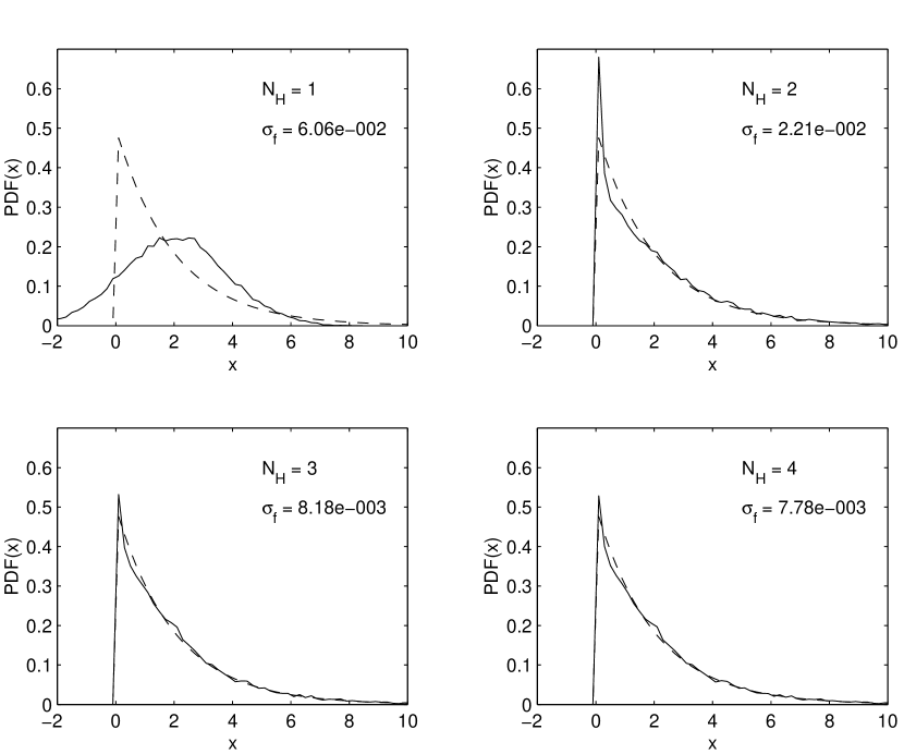
Figure 4: Approximation of the $\chi_{2}^{2}$ PDF obtained through the Hermite polynomial expansion with $N_{H}$ ranging from $1$ to $4$. For all the examples $N=16000$. The quantity $\sigma_{f}$ is equal to $\|f_{R}-f_{r^{*}}\|$ (see text), where $f_{r^{*}}$ has been obtained via an histogram.

• the algorithm works also in case of very skewed distributions (see figure 4).

One inconvenience in using this algorithm is that $f_{R}(r)$ is only approximated and in particular situations this fact can be troublesome. For example, in case of strictly positive random fields $R({\bf t})$, it could happen that $R^{*}({\bf t})$ presents some negative values. However, if the approximation is good enough (e.g. only a few values violate the constraints), the solution to this kind of problem can be very simple (es. the reflection of the negative values to positive values).

4.3 Method of Yamazaki & Shinozuka

Figure 5 shows the subroutine Field_IDF implementing an algorithm based on an idea by Yamazaki & Shinozuka (1988). The rationale behind this code is simple and is based on an iterative procedure. As explained in section 2, the mapping (27) deforms $\rho_{X}({\mbox{\boldmath$\tau$}})\rightarrow\rho_{R}({\mbox{\boldmath$\tau$}})$, and consequentely the corresponding power spectrum $S_{X}({\bf k})\rightarrow S_{R}({\bf k})$, in a complex way. However, if one applies the transformation (27) to an initial $X^{(1)}({\bf t})$, characterized by a power spectrum $S_{X}^{(1)}({\bf k})$ set equal to the target $S_{R}({\bf k})$, it is possible to recover information on the relationship between $S_{X}^{(1)}({\bf k})$ and $S_{R}({\bf k})$ from the power spectrum $S_{R}^{(1)}({\bf k})$ of $R^{(1)}({\bf t})$. A new Gaussian field $X^{(2)}({\bf t})$, characterized by a power spectrum $S_{X}^{(2)}({\bf k})$, is then built with the aim that, after mapping (27), $S_{R}^{(2)}({\bf k})$ is closer to $S_{R}({\bf k})$ than $S_{R}^{(1)}({\bf k})$ . This operation is carried out at line $21$ of the code where the power spectrum of $X^{(i+1)}({\bf t})$ is assumed to be given by

$$S_{X}^{(i+1)}({\bf k})=C({\bf k})S_{X}^{(i)}({\bf k}),$$ (41)

with

$$C({\bf k})=\frac{S_{R}({\bf k})}{S_{R}^{(i)}({\bf k})}.$$ (42)

Through this step, $S_{X}^{(i)}({\bf k})$ is modified according to the fractional difference, $C({\bf k})$, between $S_{R}({\bf k})$ and $S_{R}^{(i)}({\bf k})$. The entire procedure can be repeated $n$ times until that $S_{R}^{(n)}({\bf k})$ is a good approximation of $S_{R}({\bf k})$ .

The code presented in figure 5 has been modified with respect to the original version of Yamazaki & Shinozuka. The main difference referes to the implementation of steps $15$, $19$-$20$, $23$-$25$. The task of these steps is to constrain the range of the permitted values for $C({\bf k})$. Indeed, strictly speaking, the use of such a factor is correct only within the hypothesis that the map (27) is linear. The consequence is that in many situations $C({\bf k})$ appears as a highly oscillating function with large extremes even in cases where the target $S_{R}({\bf k})$, and therefore the starting $S_{X}^{(1)}({\bf k})$, is a smooth function. Because of this fact, in general the algorithm of Yamazaki & Shinozuka converges only with moderately non-Gaussian fields. Our modification is based on the idea that, although some values of $C({\bf k})$ could be too large, they are still able to provide indications concerning the direction of the corrections to make in $S_{X}^{(i)}({\bf k})$, via equation (41), for improving the results of the iterative process. That suggests the following procedure:

1. once $C({\bf k})$ was computed, the subset ${\bf k}^{*}$ of the indices ${\bf k}$ has to be identified for which $C({\bf k}^{*})$ is larger than a threshold $1+\delta$, where $\delta$ is an appropriate value;

2. set $C({\bf k}^{*})=1+\delta$. In this way, it is possible to obtain a smoothed version of $C({\bf k})$ that maintains the original information on the direction of the correction for each frequency ${\bf k}$;

3. if after this operation it happens that ${\rm DIST}[S_{R}^{(i)}({\bf k}),S_{R}({\bf k})]\geq{\rm DIST}[S_{R}^{(i-1)}({\bf k}),S_{R}({\bf k})]$, where ${\rm DIST}[.,.]$ indicates a distance measure between the two arguments, it is necessary to rescale the parameter $\delta$ according to a prescribed schedule. This point makes it possible to avoid troublesome oscillations of the algorithm.

From our simulations, it appears that after these modifications the algorithm converges also in situations where the original method fails.

Some notes on the use of the subroutine Field_IDF:

• the first two input quantities are the phase angles, $\phi({\bf k})$, and the power spectrum, $S_{X}({\bf k})$, of a zero-mean, unit-variance, and Gaussian random field. Here, the important point is that $S_{X}({\bf t})$ is set equal to the target $S_{R}({\bf k})$.

  The third input quantity is the initial value, $\delta_{0}$, of the parameter $\delta$. Typically, $\delta_{0}=1$-$2$, but such a choice is not so critical for the final results.

  For the fourth input quantity, $\epsilon$, see below;

• in the stopping criterion, ${\rm DIST}[.,.]\leq\epsilon$, any measure of distance can be used between $S_{R}^{(i)}({\bf k})$ and $S_{R}({\bf k})$. An interesting suggestion comes from Popescu, Deodatis & Prevost (1998) that in their work use the quantity

  $${\rm DIST}[S_{R}^{(i)}({\bf k}),S_{R}({\bf k})]=\frac{\sum_{{\bf k}}|S_{R}^{(i)}({\bf k})-S_{R}({\bf k})|}{\sum_{{\bf k}}S_{R}^{(i)}({\bf k})}.$$ (43)

  Typical value for $\epsilon$ are of order of $10^{-2}$-$10^{-3}$;

• the scaling, ${\rm SCALE}[.]$, of the parameter $\delta$ can follow any schedule. In our simulations we have halved the value whenever required by the convergence check.

In the context of the astronomical applications, some limitations concerning the algorithm are:

• the target power spectrum $S_{R}({\bf k})$ must be a smooth function. That means to work with the expected power spectra of the fields (NB. in certain engineering applications this is a demanded point). Such requirement is due to the fact that the generation of $R({\bf t})$, according to the procedure implemented in the algorithm of figure 5, in practice constitutes an optimization problem. Since the rougher a function, the larger is the corresponding number of degrees of freedom that must be accounted for by an optimization procedure, a non-smooth $S_{R}({\bf k})$ will be hardly a solvable problem with the present algorithm;

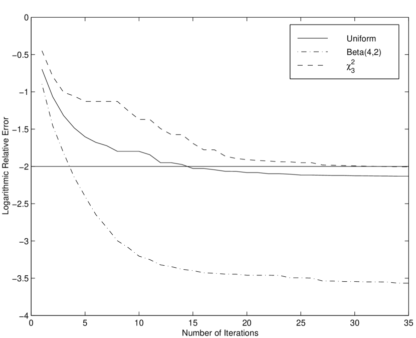
Figure 6: Convergence rate of the Yamazaki & Shinozuka method concerning some type of non-Gaussian fields: Uniform (skewness= $0$, kurtosis= $-1.2$), $\chi^{2}_{3}$ (skewness= $1.63$, kurtosis= $4$) and Beta(4,2) (skewness= $0.47$, kurtosis = $0.38$).

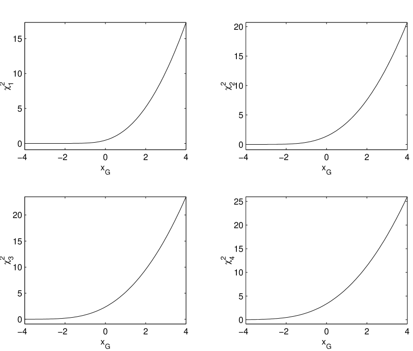
Figure 7: Mapping (27) concerning the $\chi^{2}$ distribution with $1$-$4$ degrees of freedom.

• although the algorithm is more robust than the original version of Yamazaki & Shinozuka, it still presents convergence difficulties in case of PDFs very different from the Gaussian one (see figure 6). In particular, the most serious problems concerns very skewed distributions. The reason can be understood from the figures 7a-d, where the mapping (27) is presented for four distributions $\chi^{2}_{d}$ with $d=1$-$4$. The first two distributions represent situations that the algorithm is not able to solve, the third one corresponds to a difficult case, whereas the last distribution can be easily handled with. It is easy to see that the most problematic situations concern the mappings where a large portion of the domain of the Gaussian random variable is projected onto an almost constant value. The reason is that at the i-th iteration of the algorithm, the updated $R^{(i)}({\bf t})$ is calculated on

  the basis of $X^{(i)}({\bf t})$. However, although $X^{(i)}({\bf t})=X^{(i-1)}({\bf t})+\Delta^{(i-1)}({\bf t})$, it can happen that $R^{(i)}({\bf t})\approx R^{(i-1)}({\bf t})$ since $F^{-1}_{R}\{F_{X}[X^{(i-1)}({\bf t})+\Delta^{(i-1)}({\bf t})]\}\approx F^{-1}_{R}\{F_{X}[X^{(i-1)}({\bf t})]\}$. In this case, the subsequent iterations will be not able to further improve the result.

  Another problem was recently identified by Deodatis & Micaletti (2000): after the first iteration the field $X^{(i)}({\bf t})$ is no longer strictly Gaussian and therefore the mapping (27) will not give a $R^{(i)}({\bf t})$ with the correct marginal distribution. These authors provide a modified version of the original algorithm of Yamazaki & Shinozuka where, after the first iteration, $F_{X}$ is substituted by an empirical distribution of $X^{(i)}({\bf t})$. Actually, such a method works well also in case of very skewed distributions and/or non-smooth target power spectra. Unfortunately, it is very expensive with respect to computational time which makes its use problematic in practical situations (e.g. simulation of sizeable random fields);

• in the case of homogeneous and isotropic N-dimensional random fields, it is necessary to work in the N-dimensional Fourier domain. Furthermore, the entire procedure must be restarted for each new simulation.

In spite of these problems, the algorithm described in this section maintains a certain interest since, contrary to other techniques, it can be easily adapted for the simulation of vector-valued random fields (Popescu, Deodatis & Prevost, 1998).

4.4 Fixing the Mean and the Variance

In all the methods presented in the previous sections, the mean and the variance of $R({\bf t})$ are fixed by $F_{R}(r)$. However, without modifying the correlation structure, one can force $R({\bf t})$ to have a given mean $\mu_{*}$ and a variance $\sigma^{2}_{*}$ by means of the following transformation

$$R_{*}({\bf t})=\mu_{*}+\frac{R({\bf t})-\mu_{R}}{\sigma_{R}}~{}~{}\sigma_{*}.$$ (44)

5 SOME POSSIBLE APPLICATIONS

As already reported in the Introduction, the numerical simulation of non-Gaussian random fields can be used in understanding many both experimental and theoretical physical problems.

Hot topics in Astrophysics and Cosmology, where the techniques described in this work find quick applications, can be easily identified as:

• the simulation of continuous maps to match the properties of sky backgrounds. For instance, very deep maps of the extragalactic IR sky from space are plagued by the presence of Galactic Cirrus emission and at very small scales from source confusion;

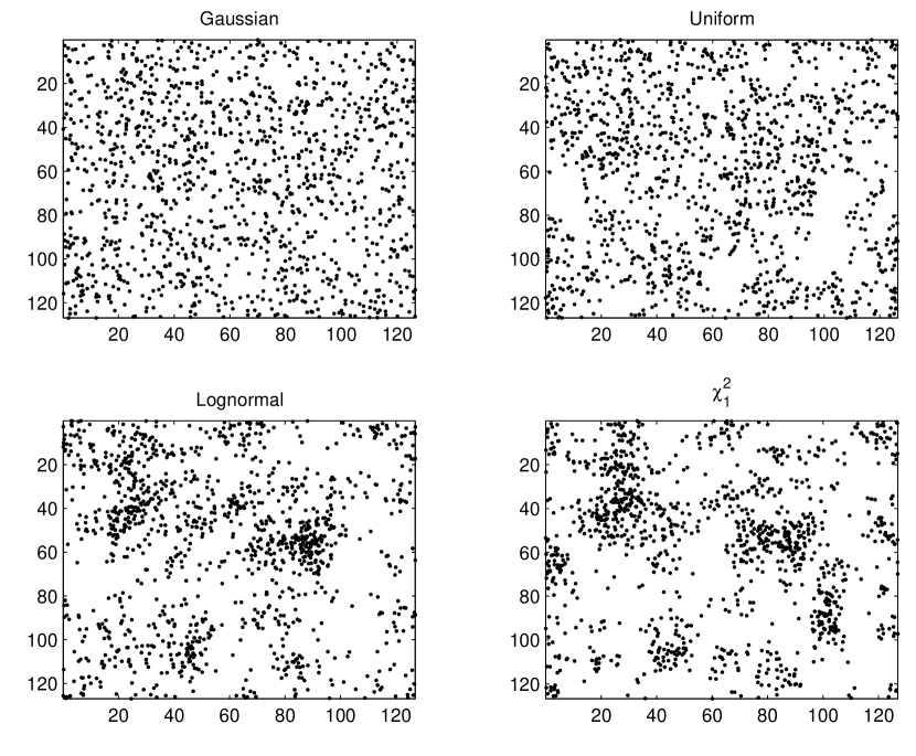
Figure 8: Point processes obtained from the non-Gaussian random fields of figure 1.

• the generation of non-Gaussian initials conditions for the N-body simulations (see figure 8). Indeed, these conditions can be obtained by interpreting a non-Gaussian random fields as a density field. In reality, such approach is not new. However, in the past the initials conditions were simulated by using only specific distributions functions as, for example, the Lognormal (Moscardini et al., 1991; Coles & Jones, 1991) and the Chi-Square (Scoccimarro, 2000) ones;

• the reconstruction of the missing parts of experimental maps (e.g. angular distribution of IRAS galaxies). Indeed, it is sufficient to transform the non-Gaussian field in a Gaussian one via the inverse of the mapping (27), to carry out the desired reconstruction through one among the many techniques available for the Gaussian case (e.g. Rybicki & Press (1992)), and then to trasform back the resulting field via the mapping (27). This techniques is described in detail in Sheth (1995) but, again, it is specialized to the Lognormal case.

6 A PRACTICAL EXAMPLE

The approach presented in this paper is going to be used to simulate the FIR sky as it will be observed by the HERSCHEL Satellite (Pilbratt, 2001). To mock extragalactic catalogues, built on the basis of theoretical modeling of the expected number of FIR sources, the emission from “local” (Galactic and interplanetary) backgrounds has to be added, in order to reproduce realistic observing conditions (Andreani et al. (2000) and Andreani et al. (2001)). Here, as an example, the reproduction of a typical Galactic background, starting from an observed sky region, is briefly outlined.

Figure 9a shows a sky map, observed by the ISOPHOT camera (Lemke et al., 1996) on board of the ISO Satellite (Kessler et al., 1996) at 175$\mu$m, with a projected size of roughly $24^{\prime}\times 24^{\prime}$ (Dole et al., 2001). The histogram of its values (see figure 9b) shows that the reproduction of such map requires the use of non-gaussian techniques. In particular, we have choosen the “change of variable method” with the following adjustments:

• the PDF of the pixel values of the original image is estimated via the Johnson parametric method (for details see Vio et al. (1994)). With such an approach it is possible to build the mapping (27), as well as its inverse, in closed form. That results in a much less expensive numerical cost than in case of the use of the more popular histogram (see Figure 9b);

• to infer the correlation function $\rho_{X}({\mbox{\boldmath$\tau$}})$, necessary for the numerical generation of the gaussian random field we prefer not to invert equation (6). Instead, we choose a set of forty-one equidistant values for $\rho_{X}$ in the range $[-0.2,~{}1.0]$, to determine the corresponding values of $\rho_{R}$ via the numerical integration of equation (6), and then interpolate the resulting points via a cubic-spline. In this way, again, a lot of computational effort is saved. The result is shown in figure 9c.

One of the possible simulations of the original map is shown in Figure 9d.

7 SUMMARY AND CONCLUSIONS

In this paper we have considered numerical simulation of non-Gaussian, scalar random fields $R({\bf t})$, with prescribed correlation structure $\rho_{R}(\tau)$ and one-dimensional marginal probability distribution $F_{R}$, based on the transformation $R({\bf t})=g(X({\bf t}))$ of a Gaussian random field $X({\bf t})$. In general, the definition of a function $g(.)$, able to map the standard random Gaussian variable $x$ in a random variable $r$ with the required $F_{R}$, is not a difficult task. Problems are found when the simulated fields has to have a desired correlation structure, since in general $\rho_{X}({\mbox{\boldmath$\tau$}})\neq\rho_{R}({\mbox{\boldmath$\tau$}})$. The determination of the appropriate $\rho_{X}({\mbox{\boldmath$\tau$}})$ is achieved using various techniques. The most effective method is that providing a closed relationship between $\rho_{X}({\mbox{\boldmath$\tau$}})$ and $\rho_{R}({\mbox{\boldmath$\tau$}})$. Unfortunately, this approach can be followed only in a very limited number of cases. Therefore, in the practical applications, very often it is necessary to resort to numerical techniques.

Here, we have presented three approaches: the “change of variable method”, the “Hermite expansion method” and the “method of Yamazaki & Shinozuka”. Whenever possible, the first one has to be adopted since, contrary to the other two, it is able to provide exact results. The only limitation concerning this method is that typically it requires the calculation of a large number of double integrals. In certain sitations that could be computationally too expensive. In this case, it is more convenient to use the “Hermite expansion method” since more robust and versatile than the “method of Yamazaki & Shinozuka”. This last method maintains a certain interest since it can be easily generalized for the numerical generation of vector-random fields.

Figure 3: Subroutines HermCoeff and Field_Herm.

Figure 5: Subroutine Field_IDF.

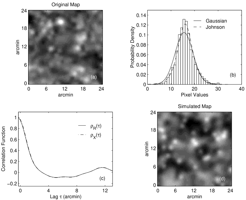
Figure 9: a) Original FIR map obtained by the ISO satellite. b) Classical and Johnson histograms of the values of the map in the previous panel. The Gaussian PDF is plotted for reference. c) Correlation function of the original map and correlation function of the Gaussian map used in the numerical experiments (see text). d) Typical non-Gaussian simulated map.

References

- Andreani et al. (2000) Andreani, P., Lutz, D., Poglitsch, A., & Genzel, R., 2000, in the Proceedings of the “The Promise of FIRST“ Symposium, ESA Special Publication (ESA SP-460). Editors G.L. Pilbratt, J. Cernicharo, A.M. Heras, T. Prusti
- Andreani et al. (2001) Andreani, P., et al. 2001, in preparation
- Blinnikov & Moessner (1998) Blinnikov, S., & Moessner, R. 1998, A&AS, 130, 193
- Coles & Jones (1991) Coles, P., & Jones, B. 1991, MNRAS, 248, 1
- Colombi (1994) Colombi, S. 1994, ApJ, 435, 536
- Contaldi & Magueijo (2001) Contaldi, C.R., & Magueijo, J. 2001, submitted (astro-ph/0101512)
- Declercq (1998) Declercq, D. 1998, Ph.D. thesis, Univ. Cergy-Pontoise (downloadable from www.etis.ensea.fr/~declercq/Research.html)
- Deodatis & Micaletti (2000) Deodatis, G., & Micaletti, R.C. 2000, submitted
- Dole et al. (2001) Dole, H., et al. 2001, A&A, in press, (astro-ph/0103434)
- Grad (1949) Grad, H. 1949, Communications in Pure and Applied Mathematics, 2, 325
- Grigoriu (1995) Grigoriu, M. 1995, Applied Non-Gaussian Processes (New York: Prentice Hall)
- Grigoriu (1998) Grigoriu, M. 1998, Journal of Engineering Mechanics, 124, 121
- Hasofer, Ditlevsen & Tarp-Johansen (1998) Hasofer, A.M, Ditlevsen, O., & Tarp-Johansen, N.J. 1998, Proceedings of ICOSSAR’97, Kyoto, November 1997 (Rotterdam: Balkema) (downloadable from www.bkm.dtu.dk/ ~od/papers.phtml)
- Herbstmeier et al. (1998) Herbstmeier, U. 1998, A&A, 332, 739
- Kessler et al. (1996) Kessler, M.F., et al. 1996, A&A, 315, L27
- Lemke et al. (1996) Lemke, D., Klaas, U., & Abolins, J. 1996, A&A, 315, L64
- Matarrese, Verde & Jimenez (2000) Matarrese, S., Verde, L., & Jimenez, R. 2000, ApJ, 541, 10
- Moscardini et al. (1991) Moscardini, L., Matarrese, S., Lucchin, F., & Messina, A. 1991, MNRAS, 248, 424
- Ogorodnikov & Prigarin (1996) Ogorodnikov, V.A., & Prigarin, S.M. 1996, Numerical Modelling of Random Processes and Fields: Algorithms and Applications (Utrecht: VSP)
- Papoulis (1991) Papoulis, A. 1991, Probability, Random Variables, and Stochastic Processes (New York: McGraw-Hill)
- Pilbratt (2001) Pilbratt, G. 2001, The FIRST ESA Cornerstone Mission, in The Extragalactic Infrared Background and its Cosmological Implications, August 2000 Manchester, eds. M. Harwit & M.G. Hauser, IAU Symp. 204, in press
- Popescu, Deodatis & Prevost (1998) Popescu, R., Deodatis, G., & Prevost, H. 1998, Prob. Engng. Mech., 13, 1
- Sakamoto & Ghanem (1999) Sakamoto, S., & Ghanem, R. 1999, Proceedings of the 13th ASCE Engineering Mechanics, The John Hopkins University, Baltimore, MD, June 13-16 (downloadable from rongo.ce.jhu.edu/emd99/sessions/sessions/allsessions.htm)
- Rybicki & Press (1992) Rybicki, G.B., & Press, W.H. 1992, ApJ, 398, 169
- Scoccimarro (2000) Scoccimarro, R. 2000, ApJ, 542, 1
- Sheth (1995) Sheth, R.K. 1995, MNRAS, 277, 933
- Slepian (1972) Slepian, D. 1972, SIAM J. Math. Anal., 3, 606
- Vanmarke (1984) Vanmarke, E. 1984, Random Fields: Analysis and Synthesis (Cambridge: the MIT Press)
- Verde et al. (2000) Verde, L., Wang, L., Heavens, A.F., & Kamionkowski, M. 2001, MNRAS, 313, 141
- Vio et al. (1994) Vio, R., Fasano, G., Lazzarin, M., & Lessi, O. 1994, A&A, 289, 640
- Yamazaki & Shinozuka (1988) Yamazaki, F., & Shinozuka, M. 1988, Journal of Engineering Mechanics, 114, 1183