THE STELLAR POPULATIONS AND EVOLUTION OF LYMAN BREAK GALAXIES

Abstract

Using deep near–infrared and optical observations of the Hubble Deep Field North from the Hubble Space Telescope NICMOS and WFPC2 instruments and from the ground, we examine the spectral energy distributions of Lyman break galaxies (LBGs) at $2.0\lesssim z\lesssim 3.5$ in order to investigate their stellar population properties. The ultraviolet–to–optical rest–frame spectral energy distributions (SEDs) of the galaxies are much bluer than those of present–day spiral and elliptical galaxies, and are generally similar to those of local starburst galaxies with modest amounts of reddening. We use stellar population synthesis models to study the properties of the stars that dominate the light from LBGs. Under the assumption that the star–formation rate is continuous or decreasing with time, the best–fitting models provide a lower bound on the LBG mass estimates. LBGs with “$L^{\ast}$” UV luminosities are estimated to have minimum stellar masses $\sim 10^{10}$ $\mathcal{M}_{\odot}$, or roughly $1/10$th that of a present–day $L^{\ast}$ galaxy, similar to the mass of the Milky Way bulge. By considering the photometric effects of a second stellar–population component of maximally–old stars, we set an upper bound on the stellar masses that is $\sim 3-8\times$ the minimum mass estimate. The stellar masses derived for bright LBGs are similar to published estimates of their dynamical masses based on nebular–emission–line widths, suggesting that such kinematic measurements may substantially underestimate the total masses of the dark matter halos. We find only loose constraints on the individual galaxy ages, extinction, metallicities, initial mass functions, and prior star–formation histories. Most LBGs are well fit by models with population ages that range from 30 Myr to $\sim 1$ Gyr, although for models with sub–solar metallicities a significant minority of galaxies are well fit by very young ($\lesssim 10$ Myr), very dusty stellar populations, $A$(1700 Å)$>2.5$ mag. We find no galaxies whose SEDs are consistent with young ($\lesssim 10^{8}$ yr), dust–free objects, which suggests that LBGs are not dominated by “first generation” stars, and that such objects are rare at these redshifts. We also find that the typical ages for the observed star–formation events are significantly younger than the time interval covered by this redshift range ($\sim 1.5$ Gyr). From this, and from the relative absence of candidates for quiescent, non–star–forming galaxies at these redshifts in the NICMOS data that might correspond to the fading remnants of galaxies formed at higher redshift, we suggest that star formation in LBGs may be recurrent, with short duty cycles and a timescale between star–formation events of $\lesssim 1$ Gyr.

Accepted for publication in the Astrophysical Journal

1 Introduction

The last few years have seen rapid advances in the study of galaxies at very high redshifts, especially at $z>2$. In a large part, this has been due to the development of simple photometric techniques to select high redshift objects by characteristic color signatures. Neutral hydrogen absorption within galaxies and from the intergalactic medium strongly attenuates flux shortward of Lyman $\alpha$ (1216 Å) and the 912 Å Lyman limit, producing a spectral “break” that provides a color signature to identify objects at high redshift. Such color selection methods have long been used to identify high redshift QSOs (e.g., Warren et al. 1987), and were latter applied to set limits on the number of star–forming, faint galaxies at $z\approx 3$ (Guhathakurta, Tyson, & Majewski 1990; Songalia, Cowie, & Lilly 1990). Using this method with a custom suite of broad–band filters, Steidel & Hamilton (1992) and Steidel, Pettini, & Hamilton (1995) established the existence of a significant number of high redshift galaxy candidates, now commonly described as Lyman break galaxies (LBGs), which were then spectroscopically confirmed to have $z\approx 3$ (Steidel et al., 1996a, b). By now, nearly 1000 LBGs have measured redshifts, providing a rich sample for studying the properties of star–forming galaxies at high redshift.

Understanding the epoch at which galaxies assembled the bulk of their stellar mass remains one of the key cosmological questions. Although new surveys are producing a growing inventory of photometric and spectroscopic data on LBGs, it is not yet clear how these objects fit into the ancestral history of the present–day galaxy population. The process of galaxy assembly depends on the particular parameters of the cosmological model, e.g., the biasing of baryonic mass relative to the underlying dark matter distribution, and the physics and feedback of star formation. In hierarchical models, galaxy formation is a continuous process driven by mergers of lower mass subcomponents over a wide range of redshifts. In other scenarios, star formation and galaxy assembly takes place on rapid timescales at high redshift, with the galaxies evolving in situ thereafter, more or less passively, to the present day. These different models predict substantially different histories and timescales for the formation and assembly of early stellar populations, especially at $z\gtrsim 1$. Observational constraints of the mass assembly history are inconclusive. The presence of old stars ($\gtrsim 10$ Gyr) in the Galactic bulge and the spheroidal components of M31 (e.g., Renzini 1999, Rich & McWilliam 2000), the existence of a population of old ellipticals at $z\gtrsim 1$ (Dickinson, 1995; Dunlop et al., 1996; Daddi, Cimatti, & Renzini, 2000), and the small scatter in the color–magnitude relation of cluster ellipticals to $z\sim 1$ (Stanford, Eisenhardt, & Dickinson, 1998) all support the picture of rapid collapse and enrichment at high redshifts, and imply that these systems formed a significant fraction of their stellar mass by $z\gtrsim 2$. Conversely, the observed clustering properties of galaxies, the steep faint–end slope of the local luminosity function (e.g., Folkes et al. 1999, and references therein), and evidence for the relative paucity of massive galaxies at $z>1$ (Cowie et al., 1996; Kauffman & Charlot, 1998) have been cited to support the hierarchical picture.

One important and unresolved issue is the stellar population content of LBGs, and their stellar and dark matter masses. Steidel and collaborators (e.g., Steidel et al. 1996b; Pettini et al. 2000) have found that the spectra of LBGs are broadly consistent with ongoing star formation, and are similar to those of local starburst galaxies. Giavalisco, Steidel, & Macchetto (1996) and Lowenthal et al. (1997) have emphasized the compact sizes of LBGs, with half–light radii of only a few kpc. The strong clustering observed for LBGs favors relatively large dark matter halo masses (Giavalisco et al., 1998; Adelberger et al., 1998). These observations are consistent with simulations (e.g., Governato et al. 1998; Baugh et al. 1998) that predict that LBGs evolve to become the bulges and spheroidal components of present–day, high–mass ($\sim\hbox{$L^{\ast}$}$) galaxies, preferentially in dense environments. In contrast, Lowenthal et al. (1997) argued that if $z\sim 3$ LBGs were to fade without continued star formation or subsequent mergers, then their sizes and luminosities would ultimately resemble those of present–day, low–mass dwarf elliptical/spheroidal galaxies. They suggest that the LBGs are possibly low–mass objects, undergoing intense, brief periods of intense star formation, which place them above the magnitude limit and within the color–selection criteria. Observations of nebular–emission–line widths for LBGs find typical values in the range $\sigma\simeq 60-120$ km s^-1 (Pettini et al., 1998, 2001; Teplitz et al., 2000a; Moorwood et al., 2000). Combined with the sizes for the galaxies, these line widths suggest virial masses $\sim 10^{10}\hbox{$\mathcal{M}_{\odot}$}$, although it is unclear whether such measurements really trace the total mass of the dark matter halos of these galaxies, which may extend well beyond the limits of the star forming, UV–bright, line emitting region.

Optical photometry has shown that the rest–frame ultraviolet (UV) continua from LBGs are typically redder than is expected from ongoing, unreddened star formation, suggesting the presence of dust (e.g., Meurer et al. 1997; Dickinson 1998; Sawicki & Yee 1998; Meurer, Heckman, & Calzetti 1999; Steidel et al. 1999; Adelberger & Steidel 2000). Nebular–line measurements for LBGs, mentioned above, have sometimes yielded estimates of star–formation rates (SFRs) that are higher than those derived from the UV continuum measurements (but see Pettini et al. 2001), again suggesting some amount of dust extinction ($A_{1700}=1-2$ mag).

Most photometric studies of LBGs have focused on their rest–frame UV light, which is dominated by short–lived, massive stars. Limited to this portion of the spectral energy distribution (SED), it is not possible to disentangle effects of metallicity, age, extinction, and past star–formation history. By extending the photometric baseline to rest–frame optical wavelengths using near–infrared (NIR) data, we may measure light from both short– and longer–lived stars, and may hope to constrain the stellar population mix in these objects. For all but the youngest galaxies, the optical rest–frame spectrum has a strong contribution from the light of later–type, main–sequence stars (A–type and later) and evolved red giants, and we may therefore expect that NIR measurements will be more sensitive to the total stellar mass, which is dominated by lower–mass stars. Also, the longer wavelengths are less affected by dust extinction that may strongly attenuate ultraviolet light.

Sawicki & Yee (1998) have studied the SEDs of 17 LBGs from the Hubble Deep Field North (HDF–N, Williams et al. 1996) using optical WFPC2 photometry augmented by ground–based infrared $JHK_{s}$ measurements from data obtained by Dickinson and collaborators (cf. Dickinson 1998). They concluded that these objects are generally quite young (median age $\sim$ 25 Myr) and highly reddened [median extinction $\hbox{$E(B-V)$}\simeq 0.3$, $\hbox{$A_{1700}$}\simeq 3.2$ mag]. Based on the derived SFRs and timescales, they concluded that the light from LBGs is dominated by short bursts of star formation and will likely only produce $\sim 5$% of the total stellar mass of a present–day $L^{\ast}$ galaxy. However, the HDF–N LBGs are typically quite faint, and the available ground–based infrared data provide measurements with rather low signal–to–noise ratios ($S/N$). Additionally, there are special challenges to matching the ground–based and WFPC2 photometry given the different resolutions and $S/N$ of the images.

In this paper, we investigate the properties of a sample of 33 LBGs with spectroscopically confirmed redshifts $2.0\leq z\leq 3.5$ drawn from the HDF–N, using new data from the Near–Infrared Camera and Multiobject Spectrograph (NICMOS, Thompson et al. 1998) on board the Hubble Space Telescope (HST). In §2, we present the broad–band photometry used for the ensemble of objects. In §3, we compare the LBG SEDs to empirical spectral templates for various galaxy types. In §4, we constrain the stellar population mix in these objects by fitting the observed SEDs with stellar population synthesis models. In §5, we discuss the implications for the galactic stellar masses and galaxy formation/evolution scenarios from the best–fit models. Finally, in §6, we present the conclusions. Throughout this paper, we use a cosmology with $\Omega_{M}=0.3$, $\Lambda=0.7$, and $h=(H_{0}/100$ km s^-1 Mpc${}^{-1})=0.7$. At the typical redshift $z\approx 2.7$ for the galaxies studied here, masses and SFRs derived from our model fitting procedure would be $\sim 50$% smaller in an Einstein–de Sitter universe with the same Hubble constant, and $\sim 10$% smaller for an $\Omega_{M}=0.3$ universe with $\Lambda=0$. We present all magnitudes in the AB system, $m_{\mathrm{AB}}=31.4-2.5\log(f_{\nu}/1\,\mathrm{nJy})$. We will denote galaxy magnitudes from the WFPC2 and NICMOS bandpasses, F300W, F450W, F606W, F814W, F110W and F160W as $U_{300}$, $B_{450}$, $V_{606}$, $I_{814}$, $J_{110}$, and $H_{160}$, respectively.

2 The Data and the Lyman Break Galaxy Sample

The original HDF–N WFPC2 observations provide high–quality photometry of faint galaxies in four bandpasses from 0.3–0.8 µm. At $z\gtrsim 2$, the Lyman limit is shifted into the WFPC2 F300W filter, permitting color selection of UV–bright star–forming galaxies with $2\lesssim z\lesssim 3.5$. The WFPC2 images sample rest–frame UV wavelengths at these redshifts ($\lambda_{0}\sim 1000-2000$ Å), and are thus primarily sensitive to light from massive young stars modulated by dust extinction. To study the photometric properties of the LBGs at rest–frame optical wavelengths, where longer–lived stars may contribute to the luminosities, where dust extinction is less severe, and where the most is known about the low–redshift galaxy population, we must observe in the near infrared. This was one of the primary justifications for our NICMOS survey of the HDF–N, in which we mapped the complete WFPC2 field of view at 1.1 µm and 1.6 µm.

The NICMOS data reach rest–frame optical wavelengths $\lambda\geq 0.4$ µm only for galaxies with $z\leq 3$. Observations at still longer wavelengths are desirable for many reasons. For galaxies at $2\lesssim z\lesssim 3.5$, the $K_{s}$–band (2.16 µm) samples the light from $\lambda_{0}\sim 5000-7500$ Å, i.e., well into the optical rest frame, providing a better “lever arm” to measure the properties of lower mass, longer–lived stars. Deep observations with HST longward of $\sim 2$ µm are impractical due to the warm telescope assembly. Therefore, we extended our data to the $K_{s}$–band using observations with the Infrared Imager (IRIM) at the KPNO 4m Mayall telescope (Dickinson, 1998; Dickinson et al., 2001). Using a technique developed by Fernández–Soto, Lanzetta, & Yahil (1999), we have analyzed the $K_{s}$ image to optimally extract photometry matched to the WFPC2 and NICMOS data. The details of this method will be presented elsewhere (Papovich & Dickinson 2001), but in summary, we use the $H_{160}$ data to create two–dimensional image templates for each object, convolve these to match the point spread function (PSF) of the ground–based data, and finally scale and fit the convolved templates to the $K_{s}$–band image to extract fluxes. This method eliminates concerns about PSF and aperture matching effects on the relative photometry between the HST and ground–based images, and permits deblending of images for objects partially merged by the ground–based seeing. We have performed detailed simulations to test the reliability of this technique and to understand the distribution of flux uncertainties. In both cases where the objects are well detected or are below the flux limit of the ground–based image, the method measures robust fluxes or upper limits. However, most of the LBGs used in this work are well detected at $K_{s}$. Although the $K_{s}$–band data are not as deep as the HST data, they provide our only access to the rest–frame optical wavelengths for $z\gtrsim 3$ galaxies.

A detailed discussion of the infrared observations and photometric catalogs will be presented in detail elsewhere (Dickinson et al. 2001, see also Dickinson 1999, 2000); a summary of the data used here is given in Table 1. Briefly, we resampled the NICMOS, WFPC2, and IRIM images to the same plate scale (0$\farcs$08 pixel^-1) and convolved the WFPC2 and $J_{110}$ images to match the PSF of the $H_{160}$  image. Our tests indicate that this PSF convolution matches point source photometry between bands to within 5% for aperture radii $>0\farcs 1$. Object detection and photometry were done with SExtractor (Bertin & Arnouts, 1996) on a combined F110W + F160W image. Relative photometry from the HST WFPC2 and NICMOS data was measured through matched isophotal apertures defined on the NICMOS images. The isophotal apertures were used for the relative colors because our tests indicate that these most closely match the $K_{s}$ photometry derived using by the template fitting method (see Papovich & Dickinson 2001). In order to correct for galaxy light outside the isophotal apertures, we then scaled the isophotal photometry for each object by the ratio of the flux within an elliptical aperture defined by radial moments of each galaxies’ F160W light profile (i.e., the SExtractor “MAG_AUTO” measurements) to the isophotal flux. The flux correction was $<20$% for nearly all of the galaxies, with a median value of 4.4%.

In order to ensure that the NICMOS and $K_{s}$ photometry reach optical rest frame wavelengths, we limit our galaxy sample to a redshift interval similar to that selected by the “$U_{300}$–dropout” Lyman break criteria. Extensive spectroscopy from the Keck telescope has measured redshifts for a subset of HDF–N LBGs (mostly from Steidel et al. 1996, Lowenthal et al. 1997, Dickinson 1998, and Cohen et al. 2000). In order to remove the redshift as a variable when fitting and analyzing the spectral energy distributions of the galaxies, we restrict our primary analysis to those galaxies with spectroscopic redshifts in the range $2.0\lesssim z\lesssim 3.5$. These objects are listed in Table THE STELLAR POPULATIONS AND EVOLUTION OF LYMAN BREAK GALAXIES. In several cases, our catalogs have split objects into separate entries that might be regarded as a single object with complex, multiple structure. For one object (HDF 2–239, using the catalog number from Williams et al. 1996) we have merged two very faint components with the brighter, main body of the galaxy. In general, however, we have left the pieces separate. In several cases, the pieces have notably different colors, and thus independent analysis may be instructive. In §4.3 we note that two galaxies have SEDs that seem inconsistent with their reported spectroscopic redshifts, and thus disregard them from the fitting analysis. We also exclude one other object, HDF 4-852.12 (NIC 824), which is apparently a broad–line AGN at $z=3.479$ (Cohen, 2001).

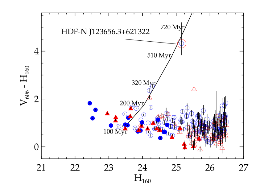
Figure 1: Color–magnitude diagram for galaxies at $2<z<3.5$ in the HDF–N. The redshift distribution has been divided into two subsamples: $1.9<z<2.7$ (blue circles), and $2.7<z<3.5$ (red triangles). Filled symbols show the spectroscopically confirmed LBGs in our sample, while open symbols are HDF–N galaxies with photometric redshifts $1.95<z_{\mathrm{phot}}<3.50$ (Budavári et al., 2000; Dickinson et al., 2001). The line shows the color–magnitude evolution as a function of age (labeled) for a $\hbox{$\mathcal{M}$}=10^{10}$ $\mathcal{M}_{\odot}$ stellar population with a $\delta$–function star–formation history, and observed at $z=2.7$. There are few photometric candidates for red, non–star–forming HDF galaxies at these redshifts. One possible candidate, the “$J$–dropout” object HDF–N J123656.3+621322 is indicated. The $S/N$ for the $V_{606}$ measurement on this object is $<2$, and thus the $\hbox{$V_{606}$}-\hbox{$H_{160}$}$ color is better considered as a lower limit. Although its nature and redshift are unknown, this object might plausibly be an example of a non–star–forming or dust–obscured galaxy in this redshift range (Dickinson et al., 2000).

Because all the objects in our subsample are bright enough for spectroscopy, they represent only the bright end of the luminosity function. They therefore may be a biased subsample, either by color (i.e., the most UV–bright and actively star–forming galaxies) or possibly by mass. However, it is important to remember that the HDF–N LBGs are on average less luminous than typical LBGs in the ground–based samples of Steidel and collaborators. In Figure 1, we show a color–magnitude diagram for all HDF–N galaxies selected from the NICMOS F110W+F160W data with $\hbox{$H_{160}$}<26.5$ and with either spectroscopic or photometric redshifts (the latter from Budavári et al. 2000, using the NICMOS and $K_{s}$ infrared photometry) in the range $1.95<z<3.5$. In principle, the infrared–selected photometric redshift sample could identify red galaxies with little or no UV flux that might be missed in optically selected Lyman break samples. However, as noted by Dickinson (2000), there are actually very few photometric candidates for galaxies in this redshift range that would not be identified in an optically selected sample. The color–magnitude distribution shows most HDF–N galaxies in this redshift range have broadly similar $\hbox{$V_{606}$}-\hbox{$H_{160}$}$ colors, and that the spectroscopically confirmed LBGs span the range of $\hbox{$V_{606}$}-\hbox{$H_{160}$}$ colors observed for the large majority of objects in the photometric redshift sample. Figure 1 includes a line indicating the colors and magnitudes expected as a function of age at $z=2.7$ for a stellar population formed in a single burst with a stellar mass $10^{10}~{}\hbox{$\mathcal{M}_{\odot}$}$. There are a few galaxies $\hbox{$V_{606}$}-\hbox{$H_{160}$}$ colors slightly redder than the majority of the LBGs (but which are still well detected in the WFPC2 data), including interesting objects such as the radio and X–ray source J123651.7+621221 (Richards et al. 1998, Dickinson et al. 2000, Hornschemeier et al. 2000, Brandt et al. 2001), with photometric redshift $z_{phot}\approx 2.6$. One very red object, the so–called “J–dropout” J123656.3+621322, is only marginally detected in the WFPC2 images and might plausibly be a reddened or non–star–forming galaxy at $z>2$, or more speculatively an object at $z>10$ (Dickinson et al. 2000). However, with this possible exception, of the $\approx 200$ galaxies with (photometric or spectroscopic) redshifts, $2.0\lesssim z\lesssim 3.5$, there are no other good candidates for relatively massive, non–star–forming HDF galaxies at $z>2$ and with ages $\gtrsim 0.3$ Gyr.

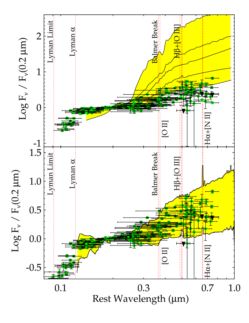
Figure 2: Ensemble photometry of the 33 LBGs compared to empirical galaxy templates. The green data points are the measured LBG fluxes from the WFPC2 ($U_{300}$,$B_{450}$,$V_{606}$,$I_{814}$), NICMOS ($J_{110}$,$H_{160}$), and IRIM ($K_{s}$) images, normalized to common flux density at $F_{\nu}(2000\;\hbox{\AA})$ (black triangles indicate upper limits). Top panel: The yellow shaded region is defined by spectral templates for ordinary galaxies from Coleman et al. (1980), spanning the range from the earliest types (elliptical), through Sab, Sbc, and Scd spirals, to the bluest, Magellanic Irregular (Im) templates. While the Im template is similar to the average LBG, the earlier–type, Hubble sequence galaxies are all much redder than any of the LBGs. Bottom Panel: The yellow shaded region spans the range of empirical starburst galaxy SEDs from Kinney et al. (1996), from the bluest [NGC 1705, $\hbox{$E(B-V)$}\simeq 0.0$] to reddest [$0.6<\hbox{$E(B-V)$}<0.7$] templates. Common spectral features are indicated by dotted red lines. The LBG SEDs fit comfortably within the envelope defined by the starburst templates.

We note a color–magnitude trend in Figure 1, in the sense that the brightest galaxies at $H_{160}$ tend to have redder optical–infrared colors. Because this is an infrared–selected, complete sample, there is no reason to think that this is due to any selection effect. To test the robustness of this correlation, we performed a Monte Carlo boot–strap test by randomly reassigning colors from the $\hbox{$V_{606}$}-\hbox{$H_{160}$}$ distribution (with substitution) to the $H_{160}$ magnitudes. We find that the observed trend is randomly reproduced with a linear slope as steep or steeper in only $\simeq 0.03$% of the Monte Carlo simulations, which supports a strong likelihood that this correlation is not obtained from random sampling. This trend might suggest that the most luminous galaxies in this redshift range are comparatively “older” (i.e., have lower ongoing SFRs for their total mass), or that they are dustier. A similar color–magnitude trend has been noted for the UV light from HDF LBGs (Meurer et al. 1999), and interpreted as a measure of varying dust content and/or metallicity.

3 Comparisons to Empirical Galaxy Spectra

The HDF–N Lyman break galaxies have significantly bluer colors than those of local spiral and elliptical galaxies. In Figure 2, we compare the SEDs of the HDF–N LBGs with empirical UV–to–optical spectral templates for local galaxies from Coleman, Weedman, & Wu 1980 (henceforth CWW). The LBG SEDs are uniformly bluer than even the actively star–forming Scd spiral galaxy template from CWW, and most are bluer than even the CWW Magellanic Irregular SED. The CWW Scd model would predict $\hbox{$V_{606}$}-\hbox{$H_{160}$}\gtrsim 2$ for $2\lesssim z\lesssim 3.5$, redder than all but a very few of the NICMOS–selected galaxies in either the spectroscopic or photometric redshift based samples shown in Figure 1. Even for a sample selected from deep infrared images, it appears that nearly all HDF–N galaxies at $2\lesssim z\lesssim 3.5$ have specific SFRs (i.e., the instantaneous, ongoing rate of star formation relative to the integrated past star formation or total stellar mass) that are higher than those of present–day Hubble Sequence galaxies. Such rapid star formation is more characteristic of that in local starburst galaxies, which are not represented among the CWW models.

In Figure 2 we also compare the LBG photometry to six empirical starburst galaxy templates (Kinney et al., 1996) with varying dust extinction ranging from $\hbox{$E(B-V)$}\simeq 0.0-0.7$. The LBGs all fall within the envelope defined by these templates, which demonstrates that their UV–optical SEDs are broadly similar to those of local starburst analogs. The UV spectra are generally redder than those of the unreddened starbursts, and there is also a spectral inflection around the Balmer break region that indicates a strong contribution to the SED from longer–lived stars (A–type and later).

We also fit all the Kinney et al. galaxy templates (five quiescent galaxy types – Elliptical, S0, Sa, Sb, Sc – six reddened starbursts, and the spectrum of the very blue, essentially unreddened starburst NGC 1705) to the SED of each LBG. The distribution of the best fitting templates is shown in Figure 3. The photometry for most of the LBGs, 19/33 ($\simeq 58$%), are best fit by starburst templates with a moderate level of dust extinction, $\hbox{$E(B-V)$}\sim 0.1-0.2$. Of the other LBGs in the sample, 10/33 of the galaxies are well fit by essentially unreddened starburst models or the extreme blue template for NGC 1705. Only 4/33 cases have best fit templates with large color excesses, $\hbox{$E(B-V)$}\gtrsim 0.25$. None of the LBGs were well fit by the quiescent galaxy templates. Based on these results, therefore, the typical LBG SED is broadly similar to local starburst galaxies with modest amounts of the dust extinction — typical UV continuum suppressions at 1700 Å on the order of, $\hbox{$A_{1700}$}\sim 0.5-1.0$ mag. These values are somewhat lower than those derived from other methods (Sawicki & Yee, 1998; Meurer et al., 1999; Steidel et al., 1999, see also §5.1).

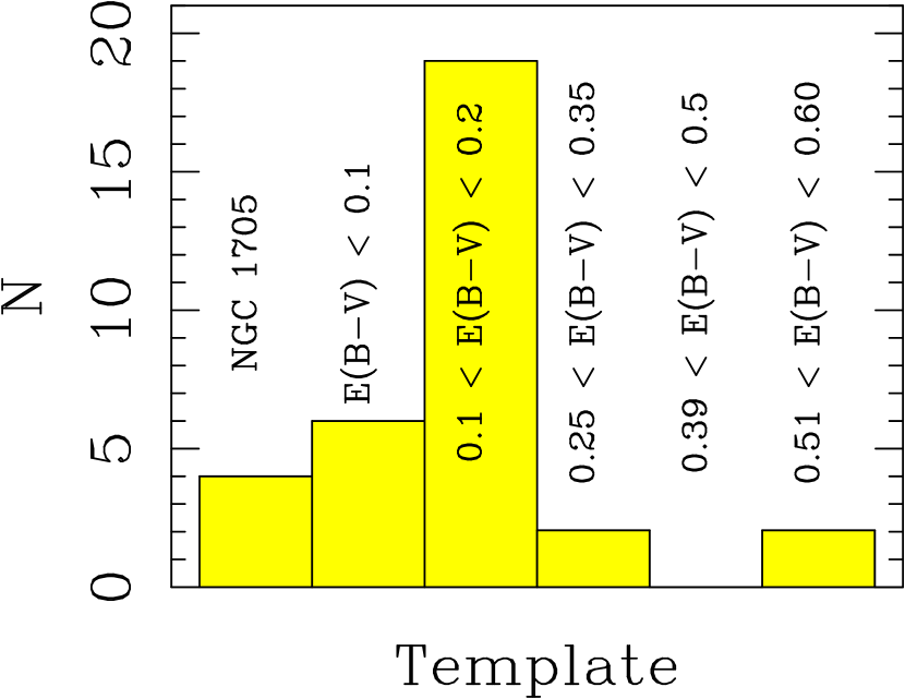
Figure 3: Distribution of the starburst galaxy template types Kinney et al. (1996) that most nearly match galaxies in the LBG sample. The columns correspond to each starburst template, as labeled. The first column refers to the very blue starburst galaxy, NGC 1705 [$\hbox{$E(B-V)$}\simeq 0.0$]. The next five columns are labeled by the range of reddening values that correspond to the averaged starburst templates.

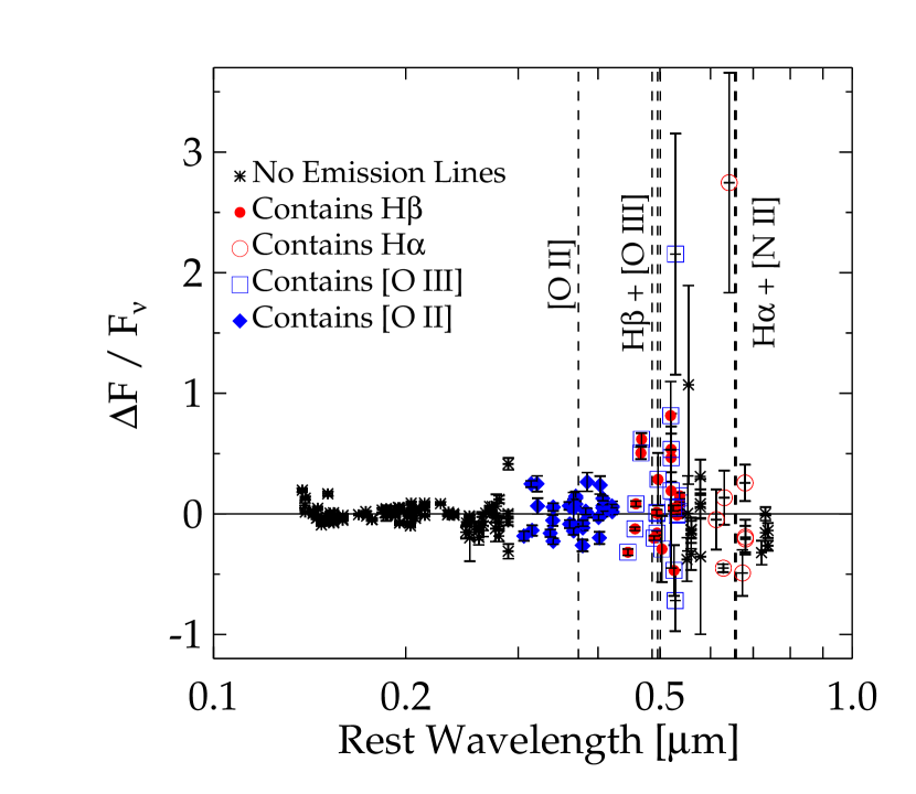
Figure 4: Residuals between the observed LBG photometry and the best–fitting starburst galaxy templates. The data points show the fractional difference between the data and model versus the rest–frame wavelength, and error bars indicate the observed flux uncertainty. Each data point is coded to indicate whether the bandpass spans a prominent emission line, as indicated in the figure.

One possible concern with the infrared LBG photometry might be the presence of a significant flux contribution from nebular emission lines, arising from heated and shocked gas associated with regions of star formation (the most common being [O II], [O III], H$\alpha$+[N II], and H$\beta$, which are labeled in Figure 2). Very strong emission lines can enhance the flux in a given bandpass and alter the galaxy colors. In several instances, strong nebular emission lines have been known to substantially affect broad–band infrared magnitudes and colors for high redshift radio galaxies (e.g., Eisenhardt & Dickinson 1992, Eales et al. 1993), although generally radio galaxies have much stronger line emission than do ordinary, star–forming galaxies. To investigate their contribution to the integrated fluxes, we consider the effect of an emission line with equivalent width $W\equiv F_{\rm line}/F_{\lambda}^{c}$, where $F_{\rm line}$ is the integrated flux in the emission line and $F_{\lambda}^{c}$ is the flux density of the continuum. Assuming a (roughly) flat continuum, the average flux density measured through a bandpass is approximately, $F_{\lambda}\simeq F_{\lambda}^{c}+F_{\rm line}\,\Delta\lambda^{-1}$, where $\Delta\lambda$ is the width of of the bandpass. This can be reexpressed as

$$\frac{F_{\lambda}}{F_{\lambda}^{c}}\simeq 1+\frac{W_{0}(1+z)}{\Delta\lambda},$$ (1)

where we substitute the rest frame equivalent width $W_{0}=W(1+z)^{-1}$. Therefore, an emission line with rest frame equivalent width $W_{0}$ introduces a magnitude increase of

$$\Delta m\simeq-2.5\log\left[1+\frac{W_{0}(1+z)}{\Delta\lambda}\right].$$ (2)

For galaxies in the redshift range of interest here, the optical nebular lines pass through the NICMOS and $K_{s}$ filters. The range of nebular emission lines observed in both the Kinney et al. local starburst templates and the Pettini et al. (2001) spectroscopic observations of $z\sim 3$ galaxies show that the equivalent width of [O III] can be as high as $W_{0}\sim 200$ Å. For the redshifts considered here, this corresponds to an increase in the observed broad–band fluxes of $\Delta m\simeq 0.2$ mag to the $H_{160}$– or $K_{s}$–bands.

We investigated the emission–line contamination by examining the residuals in the $\Delta F_{i}/f_{\lambda_{i}}$ distribution, where $\Delta F_{i}=f(\lambda_{i})-s_{i}T_{j}(\lambda_{i})$ is the difference between the observed flux through a bandpass, $i$, and the “best–fitting” Kinney et al. template, $j$. In Figure 4, we show this distribution for the LBG sample. Each data point is coded to indicate if the bandpass contains one of the strong emission lines, [O II], [O III], [N II], H$\alpha$, or H$\beta$. Properly accounting for the photometric measurement uncertainties (which are generally larger for the infrared data), the scatter for bandpasses spanning one or more strong emission lines is equivalent to that for bandpasses devoid of emission lines. To test this further, we refit the observed LBG photometry to the Kinney et al. templates with the major emission lines removed by interpolating across those wavelength intervals (i.e., [O II], [O III], H$\beta$, H$\alpha$, and [N II]). The strongest emission lines in the local starbursts have similar equivalent widths to the largest values measured for LBGs by Pettini et al. (2001). The resulting distribution of best-fitting spectra is essentially unchanged with respect to the previous results. Unless the nebular–line strengths for the HDF LBGs are significantly larger than those measured for other LBGs by Pettini et al., it seems unlikely that the emission lines have a significant effect on the spectral template fitting.

4 Comparisons with Stellar Population Synthesis Models

Although we have seen that the spectral energy distributions of LBGs are broadly similar to those of present–day starburst galaxies, we must refer to models in order to characterize their stellar content and star formation histories. Here we compare the LBG spectrophotometry to stellar population synthesis models to investigate constraints on the galaxy ages, star–formation histories, dust extinction, and stellar content. Because our photometry spans a broad range of rest–frame wavelengths (0.08–0.6 µm at the mean redshift of the sample), we are sensitive to stellar population components with a wide range of ages and mass, and to different aspects of the galaxies’ star formation histories. Meurer et al. (1999) have demonstrated that the UV spectral slope (1000-4000 Å) in nearby starburst galaxies correlates with the ratio of their far–IR to bolometric luminosities, and hence the degree of extinction for star–forming regions. The UV–to–optical flux ratio (e.g., the inflection around the Balmer/4000 Å break) gauges the ratio of early–type (OB) to late–type (A and later) stars, which is a diagnostic of the past star–formation history.

To generate model galaxy spectra, we used the newest version of the Bruzual & Charlot (1993) stellar population synthesis code (Bruzual & Charlot, in preparation, BC2000). The BC2000 models generate spectra of integrated stellar populations for a specified metallicity, initial mass function (IMF), and star–formation history as a function of the population age. This technique represents the galaxies’ stellar content as the sum of a series of isochrones as a function of time for the specified star–formation history, using theoretical evolutionary tracks to predict effective temperatures and luminosities for stars as a function of mass and age. To compute the emergent spectrum, the BC2000 code uses stellar–spectral libraries, summing over the distribution of stars present at each time step. For a further description of the BC2000 models and references, see Bruzual (2000, and references therein).

We will initially consider stellar populations formed by a single, continuous episode of star formation whose rate decays exponentially with a characteristic timescale, which we vary as a free parameter. The “age” of the galaxy is therefore defined as the time since the onset of the formation of the stellar population that dominates the observed SED. The LBG star–formation histories might, in principle, be significantly more complex than these monotonically evolving parameterizations, due to discrete events such as mergers, tidal interactions, shocks, or gas accretion. However, to model such stochastic processes would require one to invoke an infinite number of discrete, possible, star–formation histories. The choice of more complex star–formation histories would not greatly affect many of the conclusions here, which pertain to the nature of the stars that dominate the observed light in the ultraviolet and optical rest frame. Our definition of galaxy age depends to some degree on the form of the star–formation history, because stars from earlier (hence older) star–formation episodes may remain undetected (see §5.2). The exponential, star–formation histories provide a lower bound on the stellar masses of the LBGs, because they include possible models with very young ages, very active star formation, and hence the smallest values of $\hbox{$\mathcal{M}$}/L$. Thus, we should consider the stellar–mass estimates from these simple models strictly as lower limits. Below, in §5.2, we will consider the effects of a two–component star–formation history, in which the first component represents the simple, monotonic, exponentially decreasing star–formation histories as above, and the second results from a stellar population formed in an instantaneous burst at $z=1000$. Such a stellar component has a maximal $\hbox{$\mathcal{M}$}/L$ by design, and as such, we argue that the total stellar–mass estimates from these models represent a conservative upper bound on the true stellar mass of the LBGs. Therefore, using these two sets of star–formation histories, we are able to bound the possible range of the total stellar masses of the LBG stellar populations in this sample.

4.1 Model Parameters

We generated a suite of population synthesis models spanning a wide range of the physical parameter space of age, star–formation timescale, metallicity, IMF, and dust extinction. We allowed for several forms of the IMF (Salpeter, 1955; Miller & Scalo, 1979; Scalo, 1986), all of which adopt lower and upper mass cutoffs at 0.1 and 100 $\mathcal{M}_{\odot}$. We parameterized the star–formation history by adopting an instantaneous SFR of the form, $\Psi(t)\sim\exp(-t/\tau)$, where $t$ is the time since the onset of star formation, and $\tau$ is the characteristic star–formation,$e$–folding time. We considered values in the range $\tau=0.01-10$ Gyr, in quasi–logarithmic intervals, as well as a constant star–formation model (in effect, $\tau\approx\infty$.) We tracked the time evolution of the model spectra in logarithmic intervals for ages from $0.126$ Myr to $20$ Gyr.

The BC2000 models offer the choice of two sets of stellar spectral libraries. One set, primarily based on Kurucz model atmospheres (see Lejeune, Cuisinier, & Buser 1997), covers a wide range of metallicities, $Z\simeq 1/200-5$ $Z_{\odot}$. Another set uses empirical stellar spectra from the compilation of Pickles (1998), but is available only for solar metallicity. We compared results from the solar metallicity model atmosphere libraries to those from the empirical spectral libraries, and found essentially no change in the results when fitting the broad–band LBG photometry.

The metallicities of LBGs are only loosely constrained from current data. Optical and infrared spectra of the gravitationally lensed $z=2.7$ galaxy cB–58 (Pettini et al., 2000; Teplitz et al., 2000a) suggest values $\sim 1/4-1/3$ $Z_{\odot}$, and NIR spectra of several other LBGs suggest values consistent with this (Teplitz et al., 2000b; Pettini et al., 2001). This is higher than measurements for damped Lyman $\alpha$ (DLA) systems at similar redshift, which generally have metallicities $Z\lesssim 0.1$ $Z_{\odot}$ (Pettini et al., 1997; Pettini, 2000). One might reasonably expect higher metallicities for LBGs than for DLA systems at the same redshift because the former are sites of active star formation, which may rapidly enrich the surrounding medium. Therefore, we have used the stellar atmosphere models so that we were able to investigate the effects of varying metallicity on the model fitting results. However, it is important to remember that the theoretical stellar atmospheres at sub–solar metallicities are relatively untested by empirical data. Leitherer et al. (2001) have recently created a library of HST  ultraviolet spectra of LMC and SMC O–type stars, and find a fairly weak metallicity dependence for some UV line indices, but there is not yet much UV spectral information for later–type stars, nor data on the overall UV–to–optical SEDs of composite stellar populations at various metallicities. In §5 below we will note various ways in which the results of our parameter fitting depend on the model metallicities. These should be regarded with some caution, due to the current dearth of empirical calibration for the low–metallicity models.

We included dust extinction using two different prescriptions: the Calzetti et al. (2000) attenuation curve inferred from local starburst galaxies, and the Pei (1992) parameterization of the extinction curve for the Small Magellanic Cloud (SMC). The empirical Calzetti et al. starburst attenuation curve has a much “greyer” wavelength dependence in the near ultraviolet than does the SMC law. In part, this is believed to be due to geometric effects resulting from a mixed distribution of stars and dust in extended galaxies. The classical stellar reddening curve for the SMC represents a combination of absorption and scattering terms. For a galaxy, photons that are scattered but not absorbed will eventually emerge. Pei (1992) provides separate parameterizations for scattering and absorption in the SMC extinction curve, and it might be appropriate to use only his absorption terms. Instead, we have retained the full SMC extinction curve with both scattering and absorption terms, precisely because it differs most substantially from the Calzetti relation. Our motivation is to diagnose the degree to which our results for LBG fitting depend on the extinction model. In this case, the steeper UV extinction of the classical SMC law provides a useful test. In reality, however, we might expect dust extinction in LBGs to behave more nearly like the local starburst examples. Often, therefore, we will focus of our attention on results derived using the Calzetti et al. (2000) starburst extinction law. In the discussion that follows, we parameterize the effects of dust as the attenuation, $A_{\lambda}=\hbox{$E(B-V)$}k(\lambda)$, in units of magnitudes, at some wavelength, $\lambda$. At our UV reference wavelength, 1700 Å, $k(1700$Å$)=9.65$.

4.2 Fitting the Synthesis Models to the LBG Spectrophotometry

To fit the population synthesis models to the LBG photometric data, we converted the synthetic spectra to bandpass–averaged fluxes. The BC2000 code generates synthetic spectra as specific luminosity density, $\ell_{\lambda}$, in units of solar luminosity per Angstrom per unit solar mass. We transformed these to luminosity per unit frequency and applied attenuation for dust extinction,

$$L_{\nu}(\lambda_{0},t,\tau,A_{\lambda_{0}},\hbox{$\mathcal{M}$})=\frac{\lambda_{0}^{2}\,\hbox{$\mathcal{M}$}}{c\,m^{\ast}(t)}\;\ell_{\lambda}(\lambda_{0},t,\tau)\,10^{-0.4\,A_{\lambda_{0}}},$$ (3)

where $\lambda=\lambda_{0}(1+z)$ relates observed– and rest–frame wavelengths, and $\mathcal{M}$ is the total galaxy mass in stars. The BC2000 model spectra are normalized so that their total mass (gas + stars) is 1 $\mathcal{M}_{\odot}$, and the stellar–mass fraction $m^{\ast}(t)$ is provided for each time step. From this we obtain the flux density,

$$F_{\nu}(z,\lambda,t,\tau,A_{\lambda_{0}},\hbox{$\mathcal{M}$})= (1+z)\,\frac{L_{\nu_{0}}(\lambda_{0},t,\tau,A_{\lambda_{0}},\hbox{$\mathcal{M}$})}{4\pi D_{L}^{2}(z)}$$ (4)

$$\times\;e^{-\tau_{\mathrm{IGM}}(z,\lambda)},$$

where $D_{L}(z)$ is the luminosity distance (cosmology dependent), and $\tau_{\mathrm{IGM}}(z,\lambda)$ is the wavelength dependent flux suppression due to the H I opacity of the IGM at wavelengths shortward of Lyman $\alpha$ (Madau, 1995). We multiplied each spectrum with the (dimensionless) bandpass throughput function $T_{\nu}$, which is the total throughput in the sense that it includes the response from the telescope, filter, and instrument optical assemblies. Thus, we obtain integrated synthetic, bandpass–averaged fluxes,

$$\langle F_{\nu}(z,t,\tau,\hbox{$A_{1700}$},\hbox{$\mathcal{M}$})\rangle=\frac{\int T_{\nu}F_{\nu}(z,\lambda,t,\tau,A_{\lambda_{0}})\,d\nu/\nu}{\int T_{\nu}\,d\nu/\nu},$$ (5)

where we have parameterized the dust attenuation as magnitudes at (rest–frame) 1700 Å, $A_{1700}$.

Once a model has been fit to the broad band galaxy photometry, its star–formation rate $\Psi(t)=\Psi_{0}\exp(-t/\tau)$ can be determined from the model normalization. This is the intrinsic rate, i.e., the physical rate that the stellar population model is forming stars at the observed age $t$. The dust correction has already been taken into account in the template fitting procedure.

Due to the nature of the BC2000 models, only discrete values for the IMF and metallicity are available, and so we hold these parameters fixed at specific values. Although we tested a wide range of values, $Z=0.01-3.0$ $Z_{\odot}$, and several forms of the IMF, we concentrate our presentation here on models with $Z=0.2$, 1.0 $Z_{\odot}$ and Salpeter or Scalo IMFs. These metallicity values are consistent with the limited observational data on LBGs (see §4.1). As we will see below, the results of our analysis do not strongly favor any particular range of metallicity for HDF–N LBGs, although the choice of metallicity does sometimes affect the parameters of the best–fitting models. To determine the best fitting models, we allow the variables $t$, $\tau$, $A_{1700}$, and $\mathcal{M}$ to vary as free parameters. We generated a suite of $\sim 10^{5}$ synthetic models that span a wide range of the physical parameter space ($t\simeq 0.001-20$ Gyr, $\hbox{$A_{1700}$}\simeq 0.0-6.7$ mag, $\tau=0.01-10$ Gyr and $\tau\rightarrow 1000$ Gyr).

We derived best–fit models for each LBG by computing a $\chi^{2}$ statistic for each model. We defined $\chi^{2}$ for each model set of synthetic data points,

$$\chi^{2}=\sum_{i}\frac{\left[f_{\nu}^{(i)}-\langle F_{\nu}^{(i)}(z,t,\tau,\hbox{$A_{1700}$},\hbox{$\mathcal{M}$})\rangle\right]^{2}}{\sigma^{2}(f_{\nu}^{(i)})+\sigma_{\mathrm{sys},i}^{2}},$$ (6)

where the $f_{\nu}$ are the observed photometric flux densities, and $\sigma(f_{\nu})$ are the pure photometric uncertainties. The $\sigma_{\rm sys}$ terms represent systematic errors that encompasses several uncertainties, which we discuss below. Although photometry is available through seven bandpasses for all objects ($U_{300}$$B_{450}$$V_{606}$$I_{814}$$J_{110}$$H_{160}$$K_{s}$), we always exclude the F300W measurement because this point is well below the Lyman limit for all LBGs and suffers from severe IGM attenuation. The relation provided by Madau (1995) represents an average value of the IGM attenuation as a function of wavelength and redshift, but cannot account for variations in $\tau_{\mathrm{IGM}}(\lambda,z)$ along individual sight lines due to the stochastic distribution of absorbing clouds. For $z>2.5$, the F450W bandpass extends significantly blueward of Lyman $\alpha$, where variations in the Lyman $\alpha$ forest density may also affect the observed flux, and therefore we also excluded that band when fitting objects at those redshifts. By excluding these bandpasses, we prevent unknown statistical deviations in the IGM from influencing the fit.

In principle, the expected value of $\chi^{2}_{0}$ per degree of freedom should be unity. In practice, we found that the minimum $\chi^{2}$ values for the best–fitting models were generally larger than this. This implied that either our models incompletely describe the true SEDs of the LBGs, that the measurement uncertainties were larger than the simple photometric errors, $\sigma(f_{\nu})$, or that the parameter error distribution is not Gaussian (or some combination of these effects). It is not surprising that the stellar population synthesis models are incomplete, because we are forced to use discrete parameter values for metallicity and IMF. We are also restricting the range of possible star–formation histories to simple exponential models. Moreover, the population synthesis models might well have systematic inaccuracies (see e.g., Bruzual & Charlot 1993, Charlot, Worthey, & Bressan 1996, Bruzual 2000), and there are almost certainly uncertainties or inherent variations in the extinction properties (see Calzetti 1997, Calzetti et al. 2000). Finally, it is not unlikely that we have underestimated the flux uncertainties for the HST photometry. The values we have used here are based on the measured pixel–to–pixel image noise, but do not account for systematic errors in the measurements as implemented by the photometry software (e.g., issues of background determination, aperture positioning, etc.), as well as additional systematic terms due to flat fielding errors, PSF mismatching, photometric zeropoint uncertainties, etc. Many of these sources of systematic error would introduce flux deviations (either errors or differences relative to a model) proportional to the source flux itself. Using the results of image simulations that were done to analyze the errors and detection efficiency in our HDF/NICMOS catalogs (see Dickinson et al. 2001), we included an additional error term $\sigma_{\rm sys}/f_{\nu}\approx 3.5$% for the HST photometry. The $K_{s}$–band photometry was measured using a different method (§2) whose uncertainties have been extensively tested and calibrated, and thus do not include this extra term. Even with this additional uncertainty, the reduced $\chi^{2}$ values were still larger than one, and we therefore included an additional 4% systematic flux error for all bands in order to force the values of the best–fit $\chi^{2}$ per degree of freedom to be of order unity. In general, including these additional uncertainty terms does not substantially change the distribution of $\chi^{2}$ values in the model space or the results for the best–fitting model, but it does affect the mapping of the $\chi^{2}$ distribution to percentage confidence contours on the fitted parameters. Overall, it has the net effect of increasing the uncertainty on the model parameters. Therefore, we expect that the parameter constraints from our modeling are, if anything, conservative.

4.3 Constraints on the Stellar Population Parameters

In Table 3, we list the parameters for the stellar population synthesis models that best fit the observed photometry for each galaxy, i.e., the models with the minimum $\chi^{2}$. Columns 1 and 2 list the NICMOS ID number and redshift, respectively. For each LBG, there are four best models (rows) that show the results for two parameterizations of the IMF (column 4) and two metallicities (column 3). The best–fit parameters (population age, star-formation $e$–folding time, $A_{1700}$, and total stellar mass) are given in columns $5-8$. All models listed in Table 3 assume the Calzetti et al. starburst extinction law, although we have also fit SMC extinction models, and will refer to these models in the following discussion. The instantaneous SFRs associated with the best–fit model is shown in column 9. The minimum $\chi^{2}$ corresponding to the best fit is given in column 10.

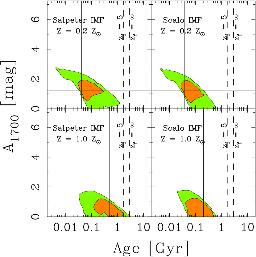
Figure 5a: Spectral synthesis model fitting results for one galaxy, NIC 503 (HDF 2-903.0, $z=2.233$), which is fairly typical of the spectroscopic LBG sample. The star–formation history used here is parameterized as decaying exponentially with $e$–folding time $\tau$. As described in the text, these models provide a lower bound on the total stellar mass of the galaxy. In each panel, we show the equivalent 68% and 95% (orange and green shaded regions, respectively) confidence intervals on various quantities plotted against stellar population age, defined as the time since the onset of star formation: (a) 1700 Å dust attenuation, (b) star–forming, $e$–folding timescale, and (c) total stellar mass. Each of the four panels corresponds to a different combination of the assumed metallicity and functional form of the IMF (as labeled). The best–fitting values (see Table 3) are indicated by the solid cross–hairs. The vertical dashed lines mark the elapsed time between the galaxy redshift and higher redshifts $z_{f}=5$ and $z_{f}=1000$. In (c), a line indicates the characteristic stellar mass of present–day $L^{\ast}$ galaxies (Cole et al., 2001).

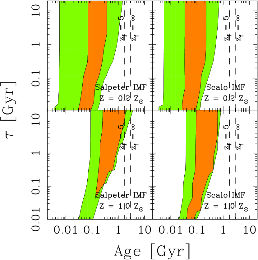
Figure 5b:

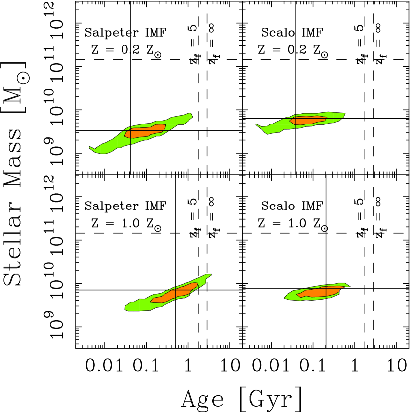
Figure 5c:

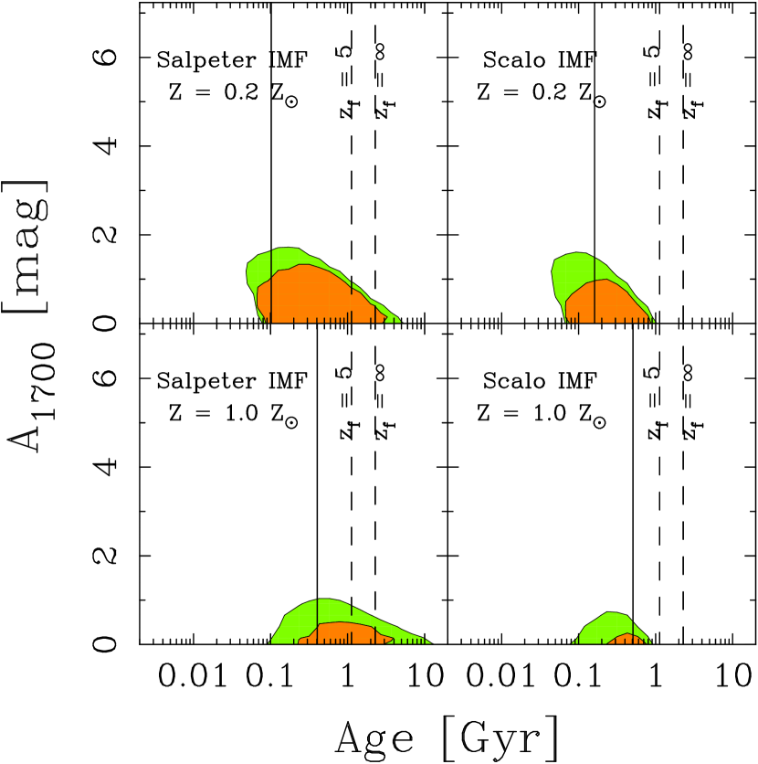
Figure 6a: Same as Figure 5a but for NIC 1352 (HDF 4-497.0, $z=2.800$), which has one of the flattest (bluest) UV spectral slopes among the galaxies in the sample.

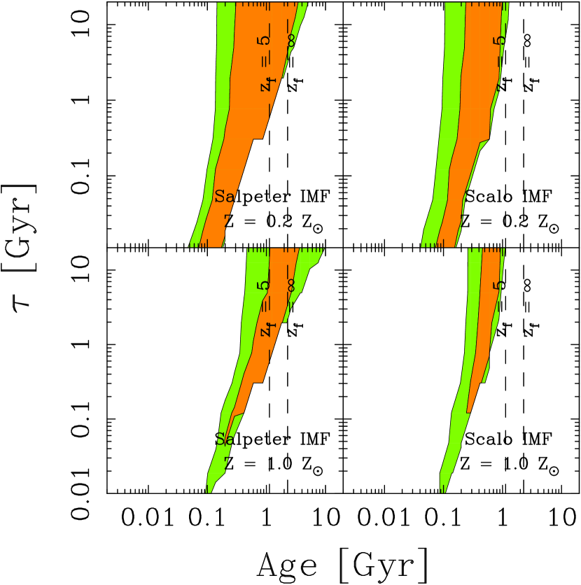
Figure 6b:

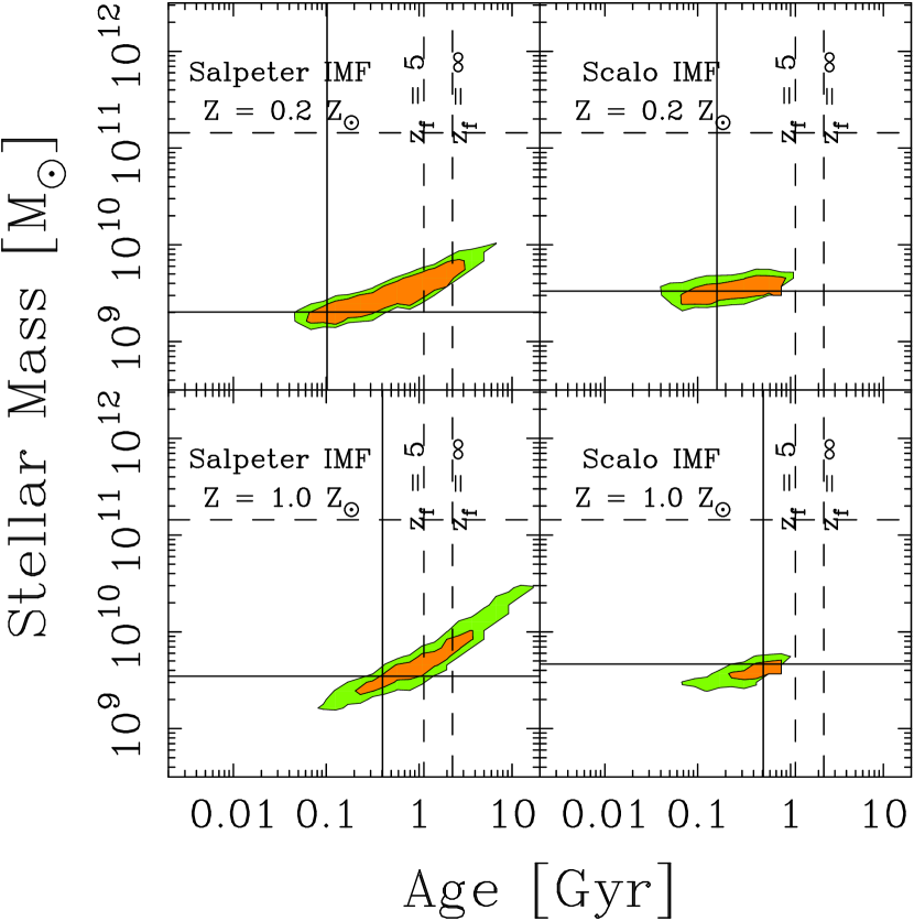
Figure 6c:

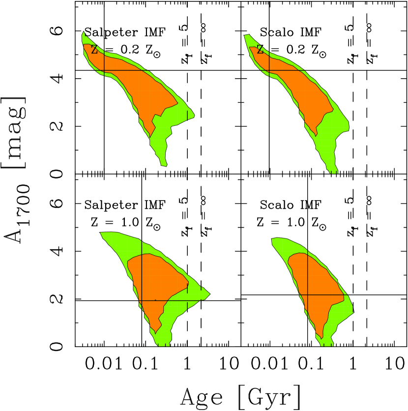
Figure 7a: Same as Figure 5a but for NIC 814 (HDF 3-93.0, $z=2.931$), one of the reddest and apparently most massive LBGs in the sample.

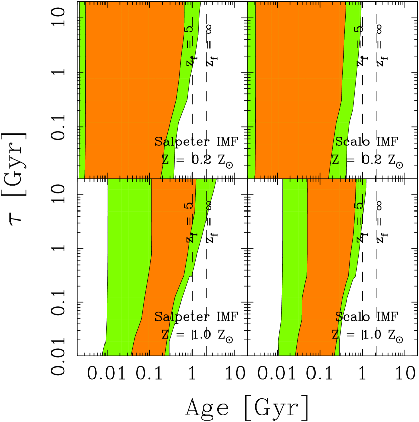
Figure 7b:

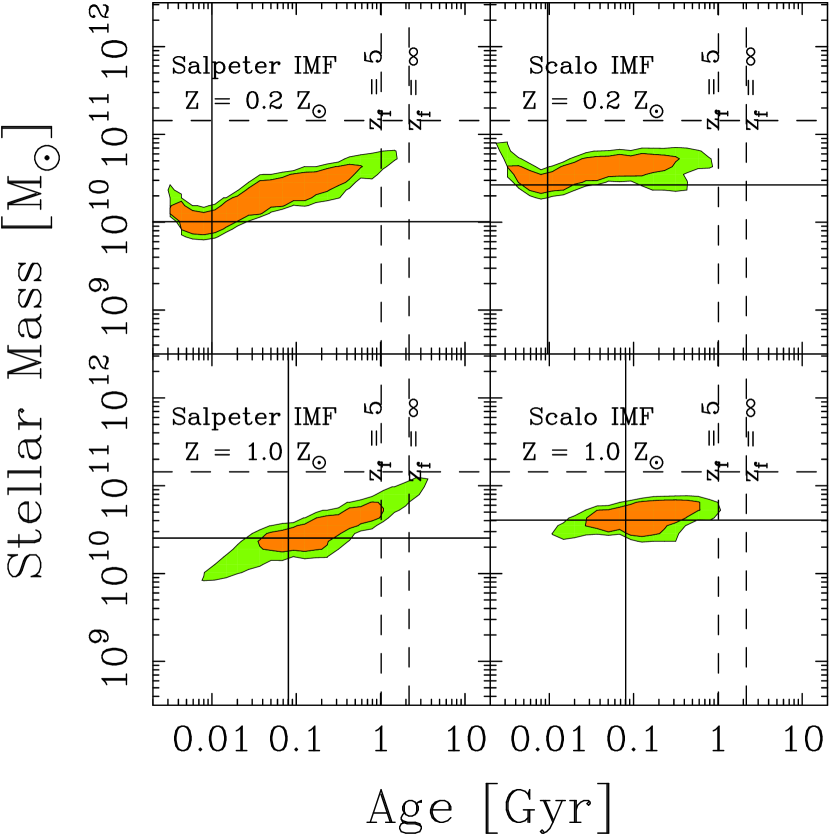
Figure 7c:

The $\chi^{2}$ statistic can be used to construct confidence intervals around the best–fit parameters. With our suite of models, we explored the likelihood that other models produce equally good fits to the data. To derive this likelihood given a best–fit model with $\chi^{2}_{0}$, we computed the probability that the correct model has a value $\chi^{2}$ that is greater than the observed $\chi^{2}_{0}$. For each model, we obtained the difference in $\chi^{2}$ between the best fit and every other model, $\hbox{$\Delta\chi^{2}$}=(\chi^{2}-\chi^{2}_{0})$. For each LBG, curves of constant $\Delta\chi^{2}$ in the multi–dimensional parameter space translate directly to confidence distributions on the parameters. To make this transformation, we performed Monte Carlo analyses using the LBGs’ flux and uncertainty distributions (including systematic uncertainties). For each galaxy, we constructed 100 synthetic realizations of the data by modulating the observed fluxes with a random amount drawn from the (normal) error distribution (including both the photometric uncertainties and the systematic errors). We then refitted the models to the synthetic data sets and derived new best–fitting models. When compared to the original best–fitting model, the curve of constant $\Delta\chi^{2}$ that encompasses some fraction of the synthetic “best–fits” corresponds directly to confidence percentages (equal to the contained fraction of synthetic best–fitting models) on the parameters of best–fits to the true data. For 100 Monte Carlo realizations, the uncertainty on the mapping of a curve of constant $\Delta\chi^{2}$ to a confidence percentage is $\sigma(X)/X\approx 7.1$% for parameter $X$.

Figures 5(a-c)–7(a-c) present examples of the types of confidence intervals we derive on the fitted parameters, shown in two–dimensional projections of the parameter space. Each figure contains a series of panels showing the parameter dependences of population age versus attenuation, age versus total stellar mass, and age versus the characteristic star–formation time scale, for assumed values for the metallicity and IMF. In each figure we also mark the lookback times to redshifts $z=5$ and 1000. In the mass–age confidence interval panels, we indicate the characteristic “$\hbox{$\mathcal{M}$}^{\ast}$” stellar mass for present–day galaxies, $1.44\times 10^{11}\;h_{70}^{-2}$ $\mathcal{M}_{\odot}$, derived by Cole et al. (2001) from their measurement of the the local $K$–band luminosity function and the optical–IR color distribution of galaxies, assuming a Salpeter IMF.

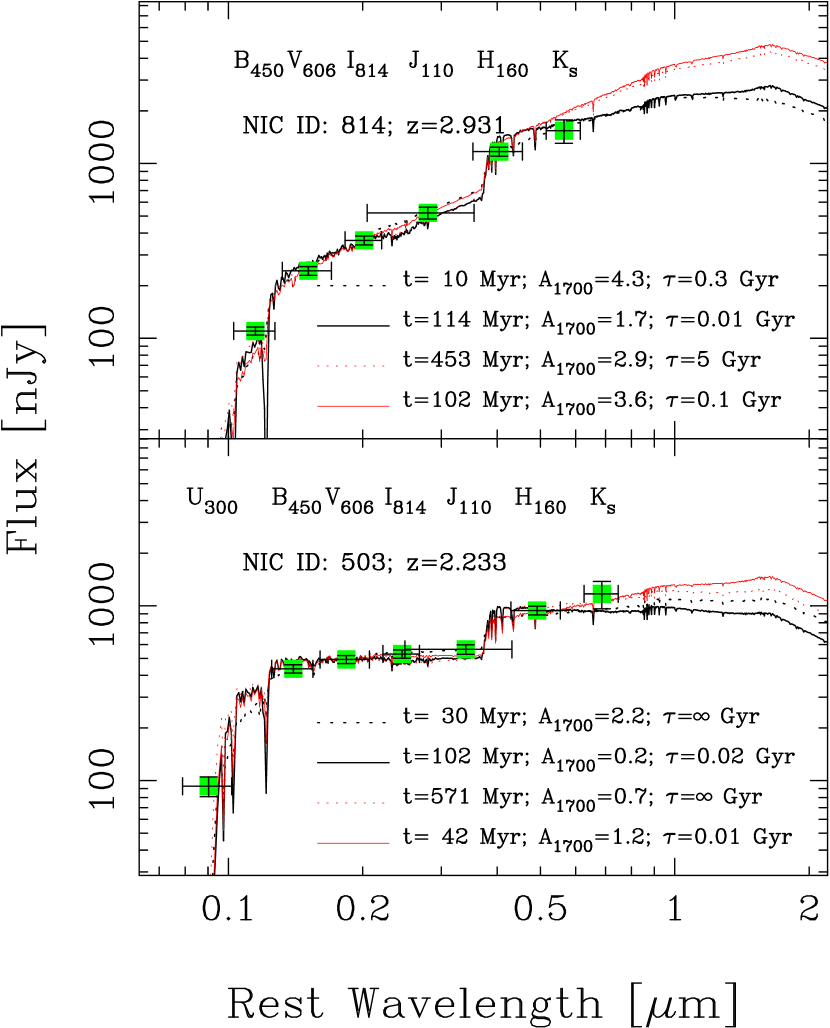
Figure 17: Model spectra fit to the photometry for LBGs NIC 503 (HDF 2-903.0) and NIC 814 (HDF 3-93.0). Each panel shows several different models drawn from within the 68% confidence region of parameter space. The model parameters are listed within each panel, see also Figures 5a and 7a. The data points (green shaded boxes) with error bars show the observed photometry. The horizontal error bars delineate the FWHM of the respective bandpasses. In the case of the WFPC2 and NICMOS data, most of the vertical photometric error bars are smaller than the symbol size.

In most cases there is a range of models that all fit the data reasonably well. In Figure 17, we show examples of model spectra, each from within the 68% confidence intervals, but with substantially differing parameters. With the available photometry, the models fit the observed SED very well in the rest–frame UV blueward of the 4000 Å and Balmer breaks. The differences between the models become larger around and redward of the $K_{s}$-band [see especially the top panel, NIC 814 (HDF 3-93.0), where the redshift is such that the $H_{160}$–band spans the Balmer break]. Thus, these models are not well differentiated. Deeper $K$–band data, and especially measurements at longer rest–frame wavelengths, e.g., from the Space Infrared Telescope Facility (SIRTF), should be quite effective in narrowing the range of possible stellar populations for galaxies at these redshifts.

Some parameters are better constrained than others, and there are some degeneracies between the fitting parameters for individual galaxies. For example, both dust and age redden the colors of the galaxies. While extinction strongly reddens the UV portion of the spectrum, the Balmer break amplitude is relatively unaffected, and thus serves as a useful age indicator, constraining the relative number of early– (OB) to late–type stars (A and later). However, even with precise NICMOS photometry, we are able to derive only rather loose constraints on age and reddening, and the confidence distributions for those parameters tend to be elongated along an axis of anticorrelation (see, e.g., Figures 5a and 7a). We note that this age–extinction degeneracy is considerably weaker when fitting with models using the SMC extinction relation.

The best parameter constraints are the derived LBG stellar–mass estimates. Based on fitting the simple star–formation histories to the observed photometry for any given LBG, the 68% range of allowable stellar masses is constrained $\sigma(\log\hbox{$\mathcal{M}$})\lesssim 0.5$ dex, with median $\simeq 0.25$ dex. In part, this is due to the high quality of the near–infrared data, which probes rest–frame optical wavelengths that are less sensitive to mass–to–light ratio ($\hbox{$\mathcal{M}$}/L$) variations due to population age or extinction. However, even in the rest frame $B$–band, $\hbox{$\mathcal{M}$}/L$ can vary substantially for stellar populations with different ages. For a given galaxy, the range of possible, intrinsic values for $\hbox{$\mathcal{M}$}/L$ is restricted by the UV–to–optical SED fitting, which constrains the age and reddening for each galaxy. Although, we have seen, these parameter constraints are somewhat degenerate, (e.g., for age versus extinction or metallicity), these degeneracies tend to cancel out in terms of their effect on the extrinsic $\hbox{$\mathcal{M}$}/L$ values, i.e., the stellar mass over the emergent (after extinction) luminosity. E.g., for spectral models that fit the photometry for a particular galaxy, the younger models will have lower $\hbox{$\mathcal{M}$}/L$, but require more extinction, which suppresses the light and raises $\hbox{$\mathcal{M}$}/L$. The reverse situation applies to older, less reddened model fits. In this way, the allowable range of $\hbox{$\mathcal{M}$}/L$ is limited, resulting in tighter constraints on the stellar mass for each galaxy (cf. Figures 5c, 6c, 7c). This method for estimating LBG stellar masses is essentially the same as that used by Brinchmann & Ellis (2000) in their analysis of field galaxies at $0<z<1$.

It is important to note that the stellar–masses derivations are based on fitting the observed LBG photometry to simple, constant or monotonically decreasing, star–formation histories. The results, therefore, are largely driven by the most luminous stellar populations (namely, the most recently formed stars). Thus, the models predict best–fitting $\hbox{$\mathcal{M}$}/L$ ratios for the stars that dominate observed light, and because these models fit the light from the youngest, highest–mass stars, we must consider these $\hbox{$\mathcal{M}$}/L$ values as lower bounds for the stellar component in these galaxies (neglecting changes to the form of the assumed IMF, see also §5.1.1). With these models, we have relatively weak constraints on the presence of any additional, older stellar components (e.g., from prior episodes of star formation), which might have substantially higher $\hbox{$\mathcal{M}$}/L$ ratios due to a predominance of lower–mass stars. Therefore, we regard the stellar–mass estimates using these simple star–formation histories strictly as minimum values for the galaxies’ total stellar mass. In §5.2 below, we consider the effects on the derived stellar parameters by adding a second, maximally old, stellar component to the simple models above.

The stellar–mass estimates do systematically depend on the functional form of the IMF and to the metallicity of the population synthesis model. Generally, increasing the model metallicities shifts the stellar masses to higher values. The size of this offset depends on the assumed form of the IMF. For a Scalo IMF, increasing the metallicity from $Z=0.2$ $Z_{\odot}$ to 1.0 $Z_{\odot}$ shifts the derived stellar masses by $\lesssim 0.1-0.2$ dex. However, for a Salpeter IMF, changing the metallicity over the same range introduces a systematic mass offset in most cases of $\sim 0.3-0.5$ dex. Furthermore, changing from Salpeter IMF to Scalo IMF models (for fixed metallicity) produces systematic stellar mass shifts of $\delta(\log\hbox{$\mathcal{M}$})=0.0$ to 0.6 dex (median $\simeq 0.2$ dex) for $Z=0.2$ $Z_{\odot}$, and 0.0 to 0.3 dex (median $\simeq 0.1$ dex) for $Z=1.0$ $Z_{\odot}$ models.

Two of the galaxies, NIC 989 (HDF 4-445.0, $z=2.500$) and NIC 782 (HDF 4-316.0, $z=2.801$), have very unusual distributions of parameter values. These galaxies have very narrow loci in the age–attenuation plots, favoring very young ages, extremely high extinction, and large stellar masses. These models appear to be somewhat unphysical, with instantaneous SFRs $\sim 30,\!000$ $\mathcal{M}_{\odot}$ yr^-1. The best–fit model spectra deviate from the observed $U_{300}$– and $B_{450}$–band data by many standard deviations. This could suggest that the published spectroscopic redshifts for these objects are erroneous. For example, NIC 782 is apparently well detected at $U_{300}$, which seems unlikely for an object at $z=2.8$. The photometric redshift analyses of Budavári et al. (2000) favor lower redshifts of $z\simeq 1.5$, and $z\simeq 1.8$ for NIC 989 and NIC 782, respectively (see also Fernández–Soto et al. 2001). We cannot exclude the possibility that these two objects have unusual SEDs that are not well fit by the models we have used, but for lack of additional information we will not consider these objects further in the remaining discussion of the LBG sample.

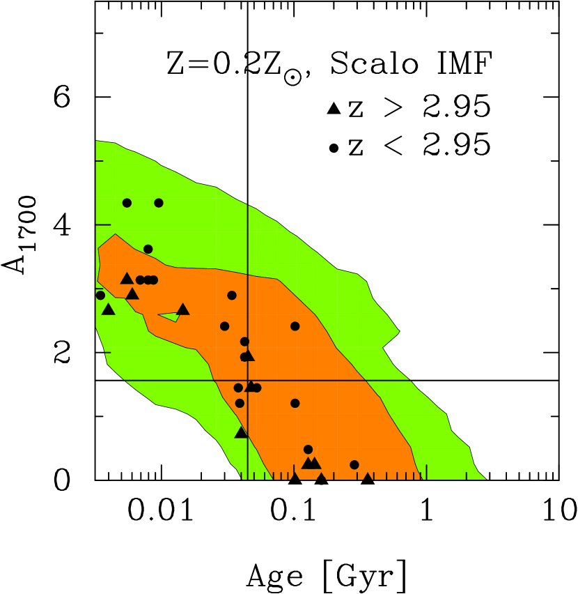
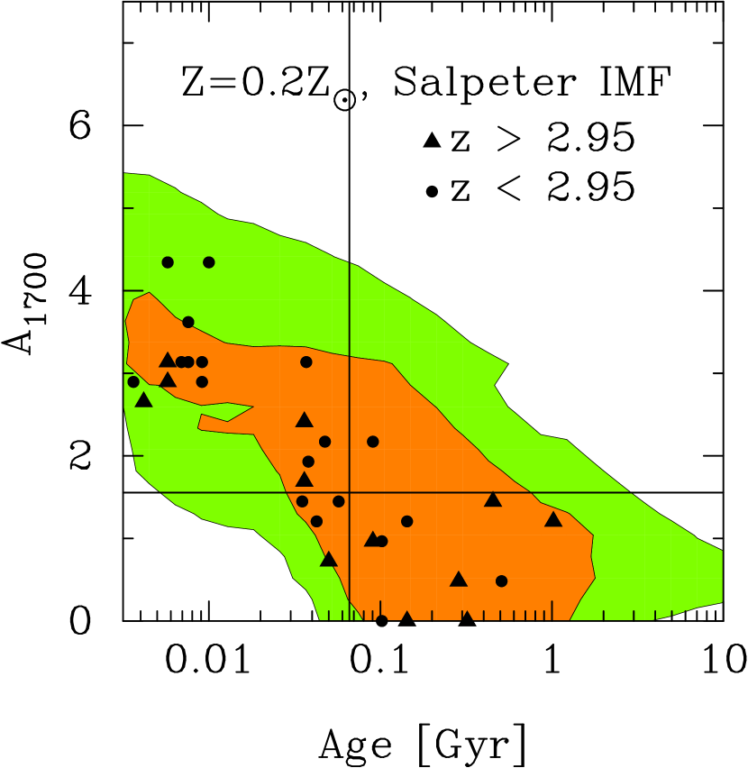
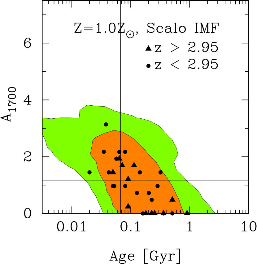
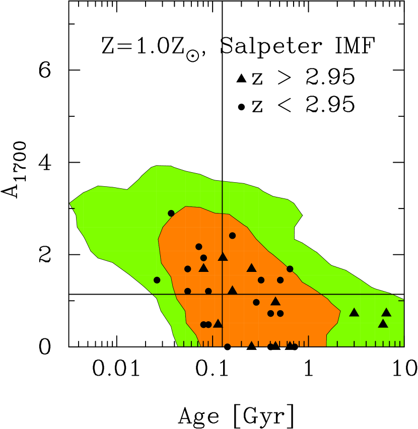
Figure 18: Composite probability distributions for the model parameters of dust attenuation versus population age for the whole LBG sample. The models used here assume the starburst extinction law. The contours represent the 68, and 95% confidence intervals averaged over the whole sample (orange and green shaded regions, respectively), and thus trace the distribution of allowable model parameters among the HDF–N LBGs. The points show the best–fit parameter values for each individual LBG, and are coded to indicate galaxies with $z<2.95$ and $z>2.95$, i.e., below and above the redshift at which the Balmer break redshifts into the $H_{160}$ filter. The cross–hairs show the (geometric) mean value for the distribution. Each panel shows results for a different combination of metallicity and IMF.

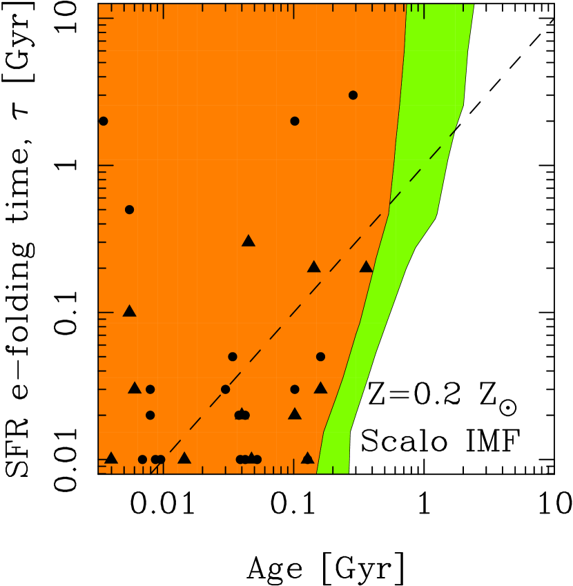
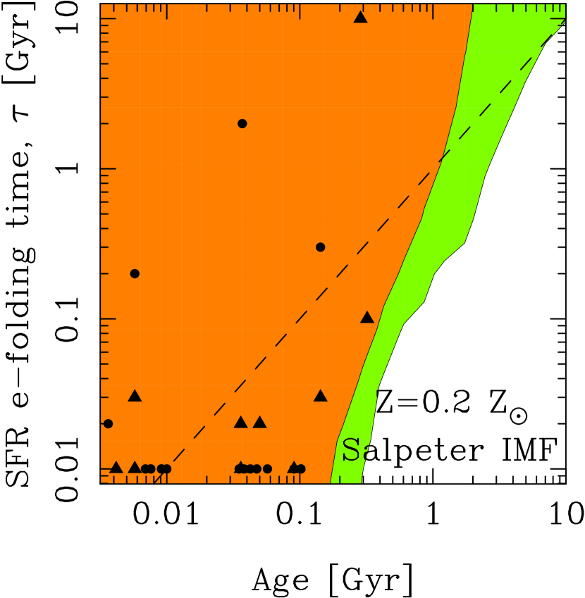
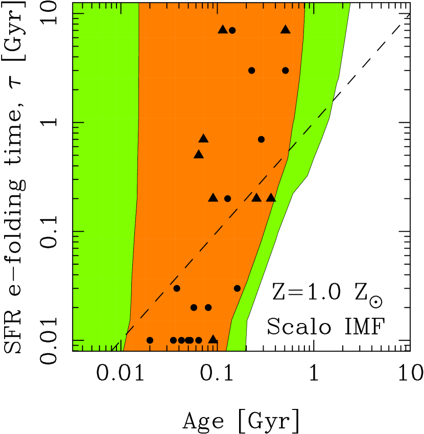
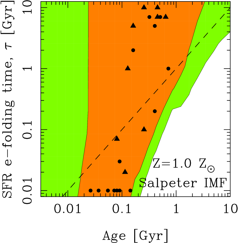
Figure 19: Composite probability distributions for the model parameters of star–forming, $e$–folding time versus population for the LBG sample, assuming the starburst extinction law. The contours and symbols are the same as in Figure 18. The dashed line indicates the one–to–one correspondence.

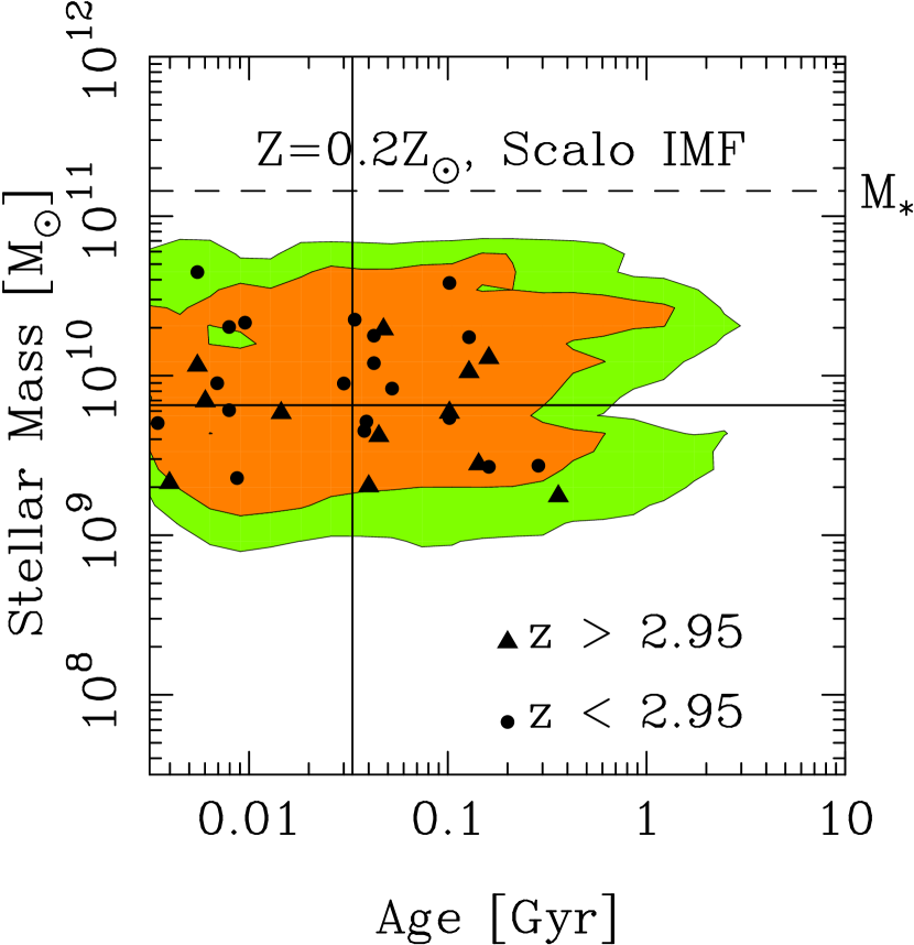
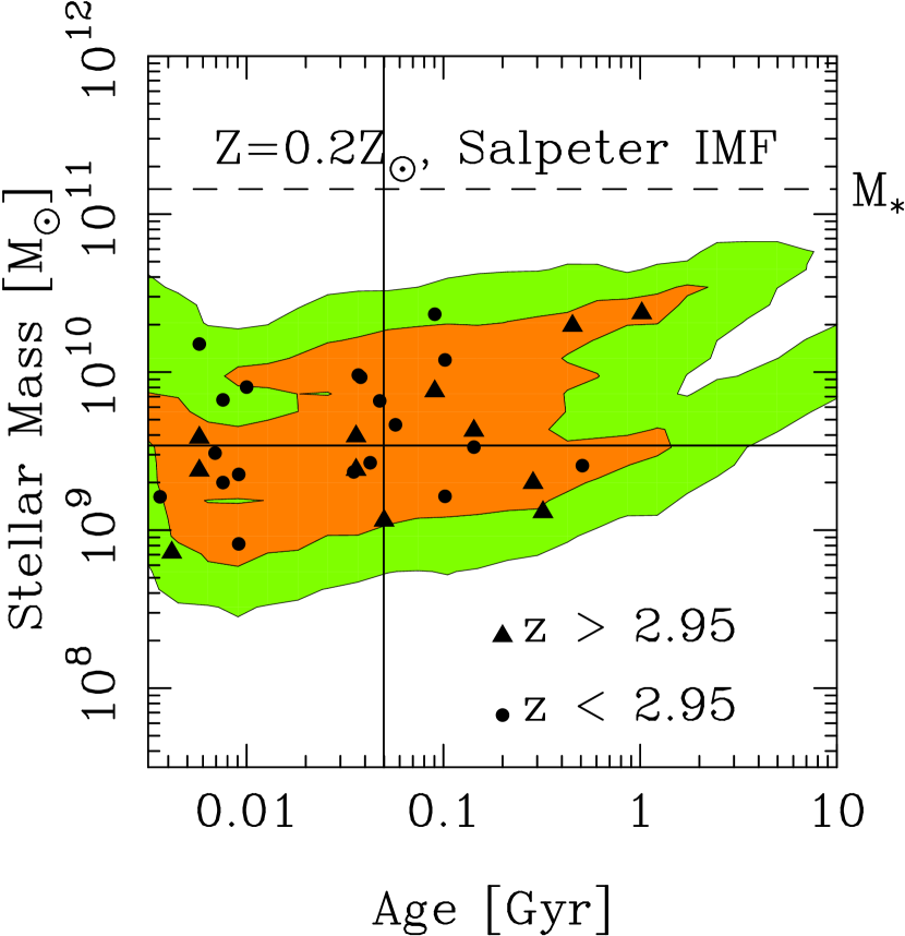
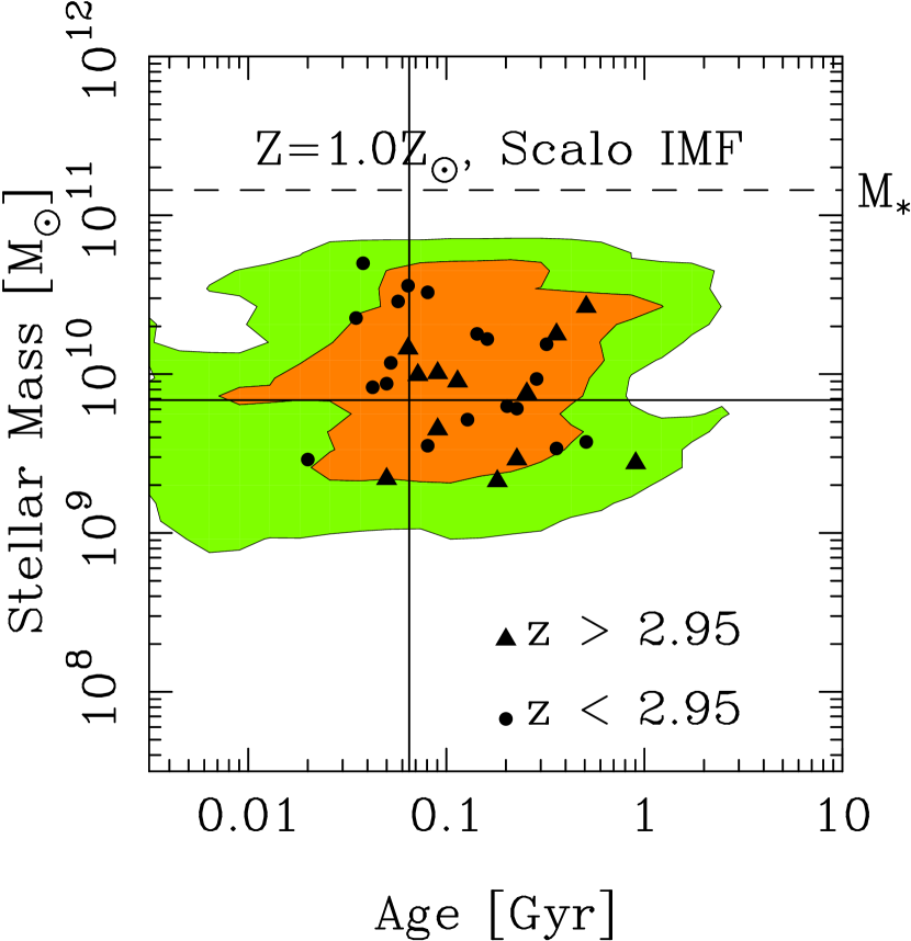
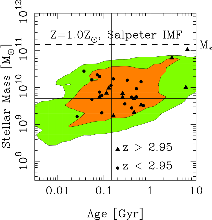
Figure 20: Composite probability distributions for the model parameters of stellar mass versus population for the LBG sample, assuming the starburst extinction law. The contours and symbols are the same as in Figure 18. The cross hairs show the (geometric) mean value for the distribution. combination.

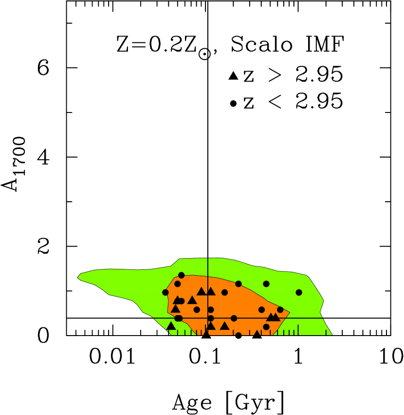
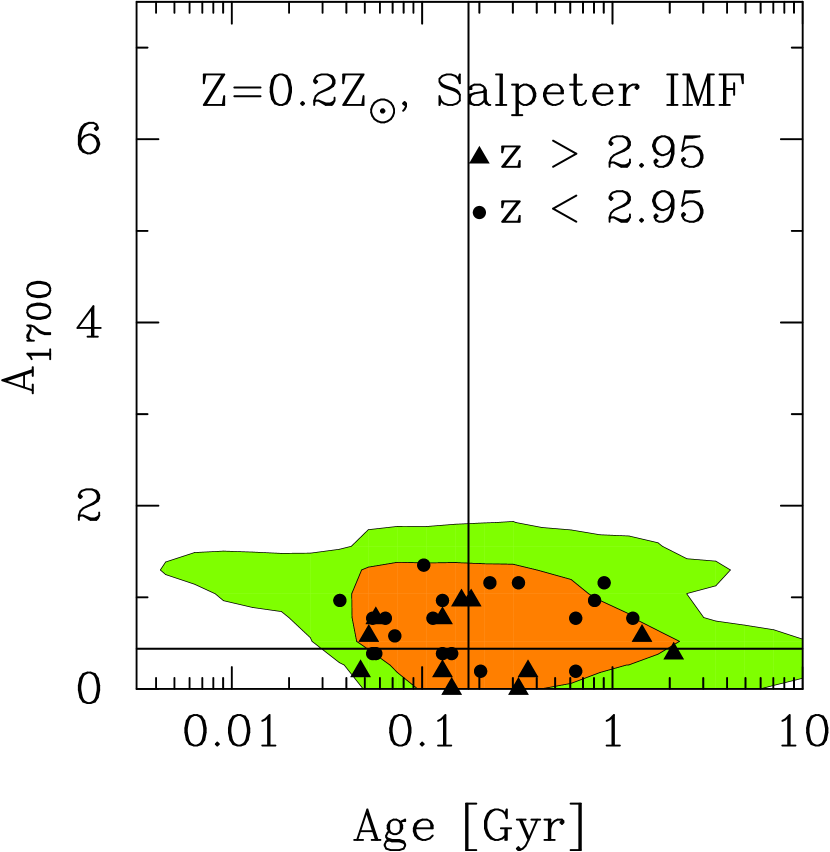
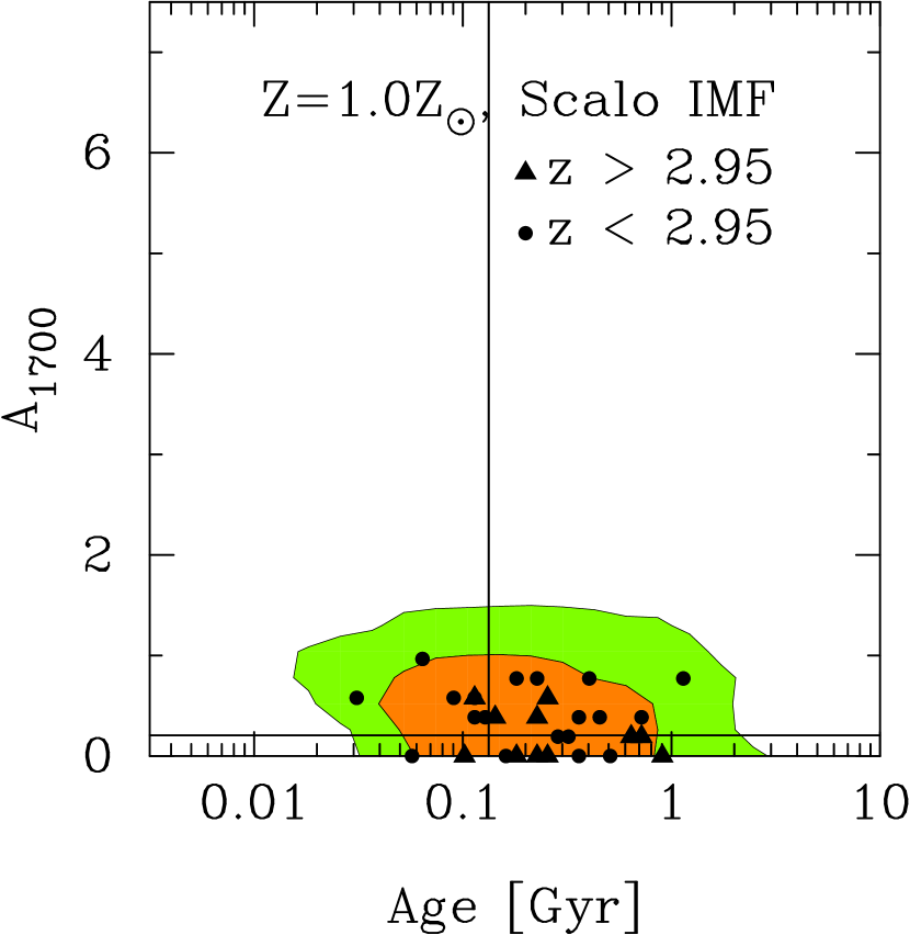
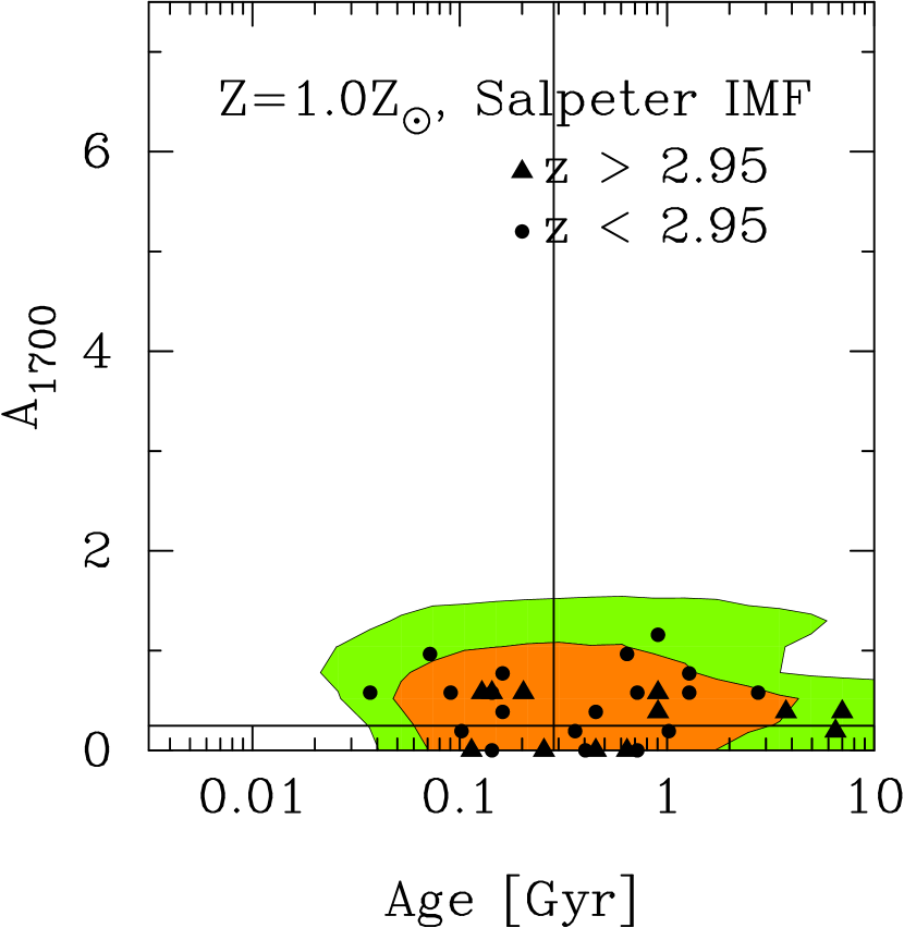
Figure 21: Same as Figure 18, but using the SMC–like dust extinction law.

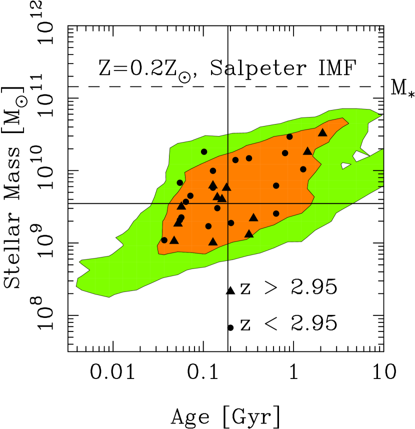
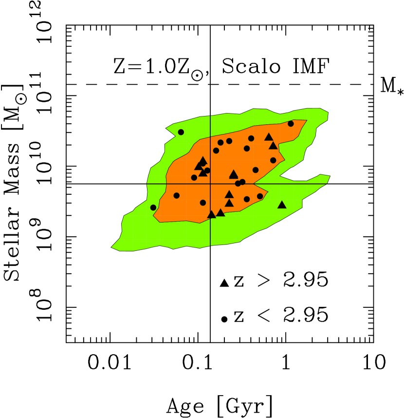
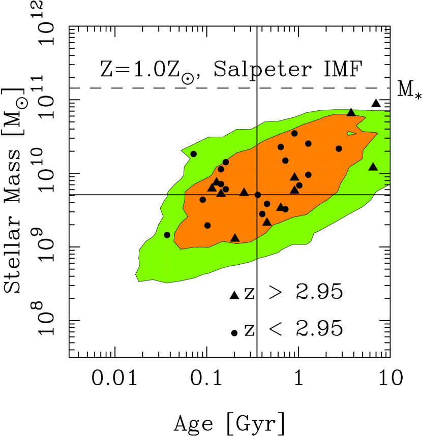
Figure 22: Same as Figure 20, but using the SMC dust extinction law.

5 Discussion

The constraints on the LBG, stellar–population parameters span a wide proportion of the available multi–dimensional parameter space. The intersection of the confidence intervals of all the LBGs in the sample generally shows that there is no region common to all the objects with any significance. There is some small overlap in the age–extinction confidence region (a compactification of the larger parameter space), which is common to all the LBGs, albeit with a very small likelihood (order of a few percent). Even so, the corresponding star–formation histories for these models vary for each object. We also note that genuine object–to–object variation is suggested from the large range of observed LBG SED colors, which is beyond what is expected from the photometric uncertainties and from simply varying only the dust content in the galaxies. Thus, this seems to suggest that there is genuine variation in the objects’ stellar–population properties. However, it is difficult (if not impossible) to prove genuine variation robustly amongst the LBGs in our sample given the current data. In this section, we use the general constraints on stellar population parameters for the LBG sample, which we use to investigate the assembly history of LBGs.

5.1 Properties of the LBG Stellar Populations

In Figures 18-22, we show combined confidence intervals for the entire sample of LBGs (excluding objects 989 and 782 for reasons given above). These plots were constructed by averaging the likelihood distributions on the fitting parameters for the individual galaxies, and thus show the favored (and disfavored) regions of the parameter space among the entire population. The best–fit values of the parameters for individual galaxies are marked by points. Different symbols code galaxies at redshifts below and above $z=2.95$. For the higher redshift objects, the 4000 Å break and 3646 Å Balmer break move through the NICMOS F160W filter bandpass, leaving only the lower–$S/N$, $K_{s}$–band data to sample rest–frame optical light, and thus making the stellar–population constraints more uncertain. In the sections that follow, we discuss the implications of the model fitting for the stellar population properties of the LBGs.

5.1.1 Initial Mass Function

The best–fitting models using any of the IMFs (Salpeter, Miller & Scalo, and Scalo) are consistent with the data. The best–fit models using the Scalo and Miller–Scalo IMFs tend to favor younger ages and slightly lower attenuation values because the steeper slope at the high mass end of these IMFs results in spectra that are inherently redder. In a detailed spectral analysis of the gravitationally lensed galaxy cB–58 ($z=2.7$), Pettini et al. (2000) show that the P Cygni profile of the C IV $\lambda$1549 line requires a significant population of stars with masses $\geq 50$ $\mathcal{M}_{\odot}$, and is inconsistent with a truncated IMF or one with a very steep high–mass slope, such as the Miller–Scalo form.

Varying the IMF lower mass cutoff would also change the derived stellar masses. The BC2000 models used here assume upper and lower mass cutoffs of $\hbox{$\mathcal{M}$}_{u}=100$ $\mathcal{M}_{\odot}$ and $\hbox{$\mathcal{M}$}_{l}=0.1$ $\mathcal{M}_{\odot}$. For a Salpeter IMF, stars with masses less than 2 $\mathcal{M}_{\odot}$ contribute typically less than $\sim 1$% of the 1700 Å luminosity. For fixed 1700 Å luminosity and fixed upper mass cutoff, the total stellar mass varies with the IMF lower mass cutoff and slope $x$, [$N(\hbox{$\mathcal{M}$})\propto\hbox{$\mathcal{M}$}^{-x}\;d\hbox{$\mathcal{M}$}$] as

$$\hbox{$\mathcal{M}$}_{\mathrm{tot}}\propto\left\{\begin{array}[]{ll}(2-x)^{-1}(\hbox{$\mathcal{M}$}_{u}^{2-x}-\hbox{$\mathcal{M}$}_{l}^{2-x})&x\neq 2\\ \ln(\hbox{$\mathcal{M}$}_{u}/\hbox{$\mathcal{M}$}_{l})&x=2.\end{array}\right.$$ (7)

So, for example, for a Salpeter IMF ($x=2.35$) with $\hbox{$\mathcal{M}$}_{l}=1$ $\mathcal{M}_{\odot}$, the total stellar mass would be 39% the mass derived with $\hbox{$\mathcal{M}$}_{l}=0.1$ $\mathcal{M}_{\odot}$.

5.1.2 Metallicity

Increasing the metallicity reddens the model SEDs. This can arise due to the combination of several effects. Higher metallicity stars have shorter main sequence lifetimes. Also, for a fixed age, higher metallicity populations have lower effective temperatures, and have stronger metallic absorption features. In general, the broad–band photometry provides little constraint on the LBG metallicities. However, the choice of metallicity can have a significant impact on the other derived parameters. As can be seen from Figures 18 and 20, increasing the model metallicities from $0.2$ $Z_{\odot}$ to $1.0$ $Z_{\odot}$ has the effect of decreasing the required extinction while increasing the population age. This effect is seen across the entire range of metallicities we have explored, $Z=1/200$ to 3 $Z_{\odot}$. As described in §4.3 above, there is some degeneracy between age and extinction when fitting the models to the photometry. In this context, it appears that there is an interplay between the effects of metallicity, age, and extinction on the galaxy colors. The choice of metallicity changes the color of the model SED at fixed age, and the best–fitting models required to fit the photometry of a particular galaxy then tend to slide along the age–extinction anticorrelation. We caution again that the theoretical stellar model atmospheres used by the BC2000 models are relatively uncalibrated by observational data at low metallicity, and therefore any results that show a strong metallicity dependence should be regarded with caution. We also note that this age–extinction degeneracy is strong for models using the starburst extinction law, but is much weaker when the SMC law is used.

5.1.3 Star Formation History

The past star–formation histories for individual galaxies are only loosely constrained by the current data set, (see the age–$\tau$ panels in Figures 5b–7b, and also Figure 17). Generally, a large region of the parameter space is consistent with the data, especially for $t/\tau\lesssim 1$, where the SFR is roughly constant and most values provide good fits. In Figure 19, we show the mean age–$\tau$ confidence region for the LBG population. In most cases, models with $t\gg\tau$, where the current SFR is much smaller than the past average, are strongly disfavored, although a few galaxies can be fit by “post–starburst” models with ages $\sim$100 Myr (see §5.1.6). In other words, the LBGs do not appear to be UV–bright objects due to a relatively small, residual tail of on–going star formation in an older galaxy, but rather are seen when they are still in the process of forming a significant fraction of their stellar content. This result may, in part, be due to the choice of exponential, monotonically decreasing or constant star–formation histories; we consider other possible star–formation histories in §5.2 below. Although for most LBGs the star–formation timescales are only poorly constrained, we do note that for all combinations of metallicity and IMF there are a number of galaxies that are best fit by short timescale “bursts” (see Figure 19).

5.1.4 Dust Extinction

For models using the Calzetti et al. (2000) starburst extinction law, there is some degeneracy in the attenuation–age parameter confidence regions (see discussion below). For individual LBGs, the 68% confidence region typically spans $\Delta A_{1700}\sim 1.5-2$ mag, which corresponds to a range of allowable flux corrections that vary by a factor $\sim 6$ at 1700 Å. For the population as a whole (see Figure 18), the distribution of best–fit values spans $\hbox{$A_{1700}$}\simeq 0-4$ mag ($\simeq 0-3$ mag) for $Z=0.2$ $Z_{\odot}$ (1.0 $Z_{\odot}$), with only a mild dependence on the chosen IMF, but with notable sensitivity to metallicity. For low metallicity models, a number of galaxies are best fit with young ages and heavy reddening, but this is not seen when solar metallicity models are used. The probability–weighted mean UV attenuation for the LBG sample is $\langle\hbox{$A_{1700}$}\rangle=1.6$ mag (1.2 mag) for $Z=0.2$ $Z_{\odot}$ (1.0 $Z_{\odot}$). The average and range of $A_{1700}$ values derived here are similar to those derived by Steidel et al. (1999) and Adelberger & Steidel (2000) based on optical photometry for a large data set of several hundred LBGs, using the same dust attenuation law but simpler stellar population assumptions. However, the luminosity–weighted average UV–flux correction (i.e., the ratio of intrinsic to emitted luminosity summed over the whole sample) is considerably larger, a factor of $\simeq 13.8$ (4.6) for $Z=0.2$ $Z_{\odot}$ (1.0 $Z_{\odot}$) and a Salpeter IMF (and similar for the Scalo IMF). This reflects the tendency for LBGs with the largest fitted dust corrections to have the highest intrinsic UV luminosities and SFRs, a point emphasized by Meurer et al. (1999) and Adelberger & Steidel (2000). Those authors argue that this is a real trend among LBGs, and not an artifact of the extinction correction process.

If the SMC extinction law is adopted instead, the anticorrelation between age and attenuation largely disappears (Figure 21), and the tail of young and high–extinction models found with the “grey” starburst dust attenuation is absent. The allowed model extinction at 1700 Å is $\lesssim 1.5$ mag regardless of IMF and metallicity, and any correlation with population age is weak at best. Most galaxies are well fit by stellar population ages $\gtrsim 40$ Myr.

Regardless of metallicity, IMF, and dust model assumptions, models with very young ages and low dust content are strongly disfavored. Very young, unreddened star–forming regions, particularly those with low metallicity, should have UV spectra that rise (in $f_{\nu}$ units) toward shorter wavelengths. In practice, this is never observed among the LBGs: even the youngest galaxies apparently contain significant amounts of dust at these redshifts. This may suggest that the LBGs have experienced metal enrichment from a previous stellar generation, and therefore the LBG population probably are not “first–generation” objects (unless the spectra of young, low metallicity, dust–free objects are sufficiently different from the models used here). Such first–generation objects must be quite rare at these redshifts, or must pollute themselves with dust on very short timescales. Alternatively, perhaps the SFRs (and hence luminosities) of such objects are too low to allow them to be detected in the the HDF images.

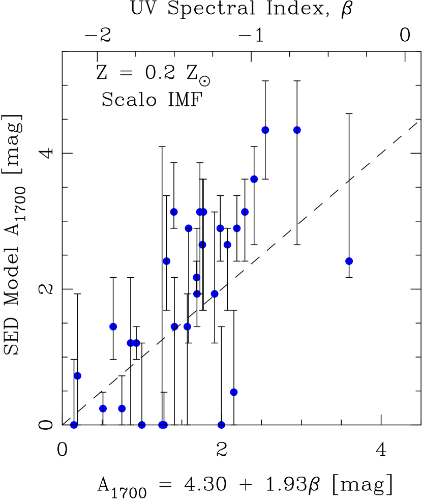
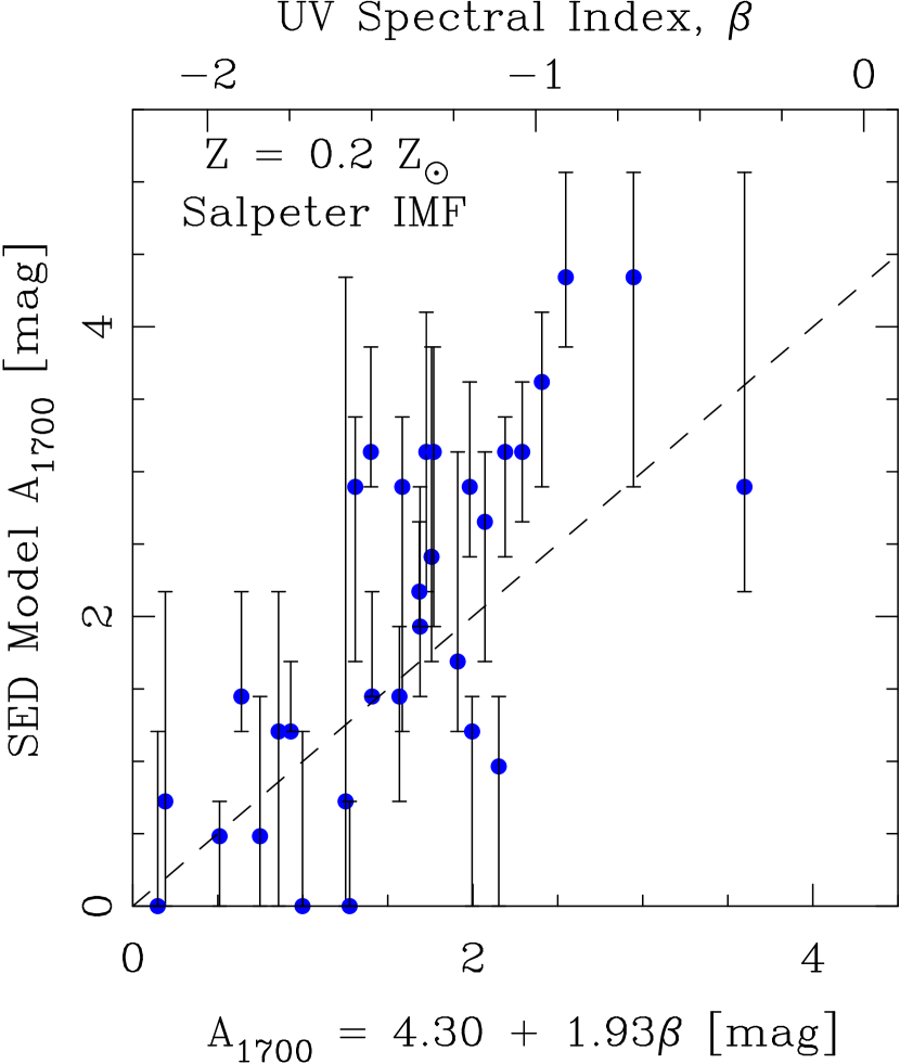
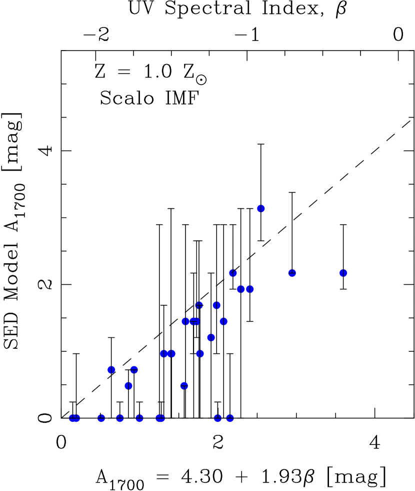
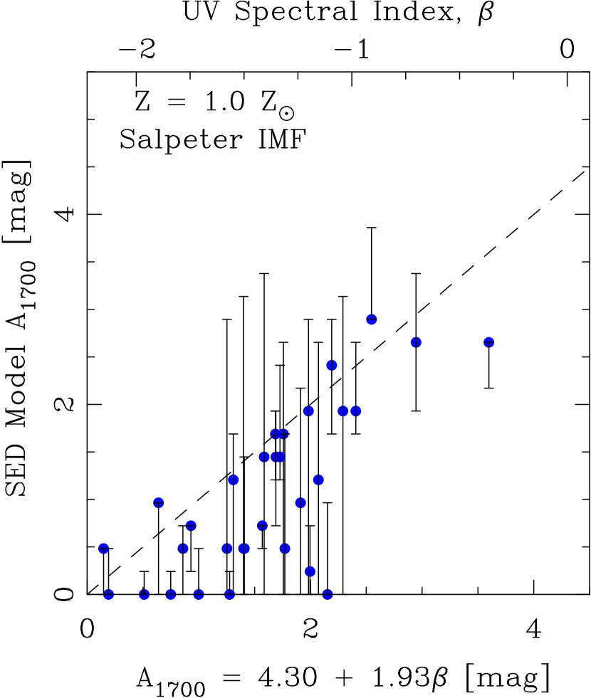
Figure 23: Comparison of the fitted SED model extinction (using the starburst attenuation law), in magnitudes at 1700 Å, with the attenuation inferred from the U–spectral index, $\beta$, alone ($f_{\lambda}\propto\lambda^{\beta}$) using the relation from Meurer et al. (1999). The $\beta$ values measured from the WFPC2 photometry are indicated along the top axis. The points and error bars in the ordinate show the best–fit values and 68% confidence intervals on dust attenuation from the population synthesis models fit to the optical–to–infrared photometry.

The extinction correction factors that we derive from the model fitting differ somewhat from those obtained by other authors using various techniques. Modelling many of the same HDF–N galaxies using ground–based NIR photometry, Sawicki & Yee (1998) find SED fits with somewhat higher median UV–flux–suppression factors, $\langle A_{1700}\rangle\simeq 2.7$ mag for $Z=0.2$ $Z_{\odot}$ models (accounting for small differences in the forms of the starburst attenuation law). The two analyses are in closer agreement at solar metallicity, where Sawicki & Yee find $\langle A_{1700}\rangle\simeq 1.4-1.9$ mag, depending on the assumed star–formation history. The differences between these analyses may be due to several factors, including the improved sensitivity of our NICMOS photometry, more accurate matching of optical to infrared photometry, allowance for a wider range of possible star–formation histories (Sawicki & Yee considered only $\delta$–function bursts and continuous star–formation models), and the use of a larger galaxy sample. Meurer et al. (1997) also found large UV–attenuation values ($\sim 15-20$) by fitting the the UV slopes of a sample of HDF–N LBGs to the starburst extinction law from Calzetti et al. (1994). However, using a revised method of a locally calibrated UV slope to far–infrared (FIR) distribution, Meurer et al. (1999) derive more modest mean extinction of factors $\simeq 5$. As noted above, the attenuations we derive are similar to those found by Adelberger & Steidel (2000) using UV rest–frame data for a larger LBG sample. Overall, the fact that the derived UV–flux attenuation depends so strongly on parameters on which we have little reliable information, such as stellar–population metallicity, leads us to believe that one must regard the quantitative results of such analyses with considerable caution, but the necessity for significant dust attenuation in many or most LBGs seems secure.

In local, UV–bright starburst galaxies, the UV–spectral slope $\beta$ ($f_{\lambda}\propto\lambda^{\beta}$) correlates with the flux emitted at far infrared wavelengths (8-1000 µm), demonstrating a close relation between UV extinction and dust reprocessing. Meurer et al. (1999) calibrate this relationship as $\hbox{$A_{1700}$}=4.30+1.93\beta$ (where we have adjusted their parameters slightly to account for a small shift in the reference UV wavelength). In Figure 23, we compare the attenuation derived from the UV–through–optical rest–frame SED model fitting to that computed from the UV slope $\beta$ alone, using the prescription of Meurer et al. (1999) to convert $\hbox{$V_{606}$}-\hbox{$I_{814}$}$ colors to $\beta$. For a given set of IMF and metallicity assumptions, there is considerable scatter ($\simeq 1$ mag) in the comparison of attenuation values. This is appreciably larger (by approximately a factor of two) than uncertainty that results from random and systematic errors in deriving $\beta$ from UV–to–FIR flux ratios (see Meurer et al. 1999). The uncertainty in $A_{1700}$ can produce substantially differing UV–flux correction factors (by an order of magnitude in flux), which directly affects the inferred SFRs (see discussion below). In some cases, galaxies with $\beta$ values that predict $\hbox{$A_{1700}$}\simeq 0.5-2.5$ mag can be fit by models requiring negligible extinction. For these objects, the full–SED model fitting would suggest that the UV–spectral slope is due to an aging stellar population rather than dust. There are also systematic offsets in the derived attenuations, depending mainly on the choice of metallicity for the population synthesis models. The lower metallicity models are bluer, and thus require more reddening to match the observed colors. On average, the best–fit values of $A_{1700}$ for the $Z=0.2$ $Z_{\odot}$  synthesis models are greater than those predicted from the UV slope alone by $\delta(\hbox{$A_{1700}$})\simeq 0.35$ mag (0.20 mag) for Salpeter (Scalo) IMF, while the solar metallicity models nearly always result in attenuation values lower than the $\beta$ predictions by $\simeq 0.6$ mag for both Salpeter and Scalo IMFs. Therefore, we emphasize that while it may be justifiable to apply an average flux correction to a galaxy ensemble, there are very likely large uncertainties, both random and systematic, when making extinction corrections to individual objects.

5.1.5 Stellar Population Age

As we have already noted, there is some degeneracy between age and extinction when fitting models to the broad–band LBG photometry (see, e.g., §4.3 and Figures 5a and 7a). A similar trend is seen for the composite distribution in Figure 18. It is not clear how much of this anticorrelation can be explained by the combined effect of the parameter degeneracies for individual galaxies, or whether there is some real tendency for younger galaxies to have more extinction. This might not be unexpected, because young star formation within our own Galaxy tends to be highly dust–obscured, and at later times, stars may blow away dust or migrate from their dusty birthplaces. On the other hand, one might expect very young galaxies to be relatively free of dust and metals, unless these were produced during previous episodes of star formation, before the birth of the current generation of stars.

As can be seen from the composite probability plots (Figure 18), the best–fit solar metallicity models span an age range of $30\;\mathrm{Myr}\lesssim t\lesssim 1$ Gyr. The upper range of population ages is similar for both low ($Z=0.2$ $Z_{\odot}$) and high (solar) metallicity models, but the low metallicity models exhibit a tail of solutions with very young ages (down to $\sim 4$ Myr) and high extinction, $\hbox{$A_{1700}$}\sim 3$ to 4 mag with the Calzetti et al. dust model. As discussed above in §5.1.2, the low metallicity models are intrinsically bluer, and thus require more extinction to fit the observed colors at a fixed age. It is notable that the fitting solutions with very young ages and high extinction appear only when using the starburst attenuation law, which has a rather “grey” wavelength dependence. Fits with the steeper SMC dust law avoid this young and heavily reddened region of parameter space.

Although the population fitting with low metallicity models allows very young ages ($\lesssim 10^{7}$ yr), these timescales may be somewhat unphysical based on the kinematics and linear size scales observed for LBGs. Nebular–emission–line widths of $\sigma\simeq 60-120$ km s^-1 have been measured for several LBGs (Pettini et al., 1998, 2001; Teplitz et al., 2000a; Moorwood et al., 2000). The objects in our sample typically have physical diameters of $3-10$ kpc. Attributing the emission–line widths to virialized motions, the corresponding dynamical timescales for these galaxies are $t_{\mathrm{dyn}}\sim 10^{7.5-8}$ yr. This may arguably set a lower bound on the time required for star formation to propagate across the galaxies, and thus on the age of their stellar populations. Therefore, these solutions are possibly disfavored even if formally allowed by the SED fits, unless one invokes an unusual geometry in which the star–formation regions and nebular emission lines do not originate in identical regions. In §5.1.6 below, we consider constraints on these solutions from limits on sub–mm emission in the HDF–N.

The geometric mean age for the composite distribution is $\simeq 70$ Myr (120 Myr) for models with metallicity 0.2 $Z_{\odot}$ (1.0 $Z_{\odot}$) and Salpeter IMF. For Scalo IMF models, the distributions have slightly lower mean ages, $\simeq 40$ Myr (70 Myr) for 0.2 $Z_{\odot}$ (1.0 $Z_{\odot}$) metallicity. For the solar metallicity, Salpeter IMF model fits, three galaxies have best–fitting model ages $t\gtrsim 1$ Gyr, resulting from their moderately red $\hbox{$H_{160}$}-K$ colors and model fits implying little or no dust extinction. All three galaxies, however, are at $z>3.2$, where only the $K_{s}$ data reaches rest frame $\lambda>4000$ Å, and for one object (NIC 284, by far the faintest object in the sample), the photometry provides only a weak upper limit to the $K_{s}$ flux. For this reason, the possible older ages for these galaxies must be regarded with caution.

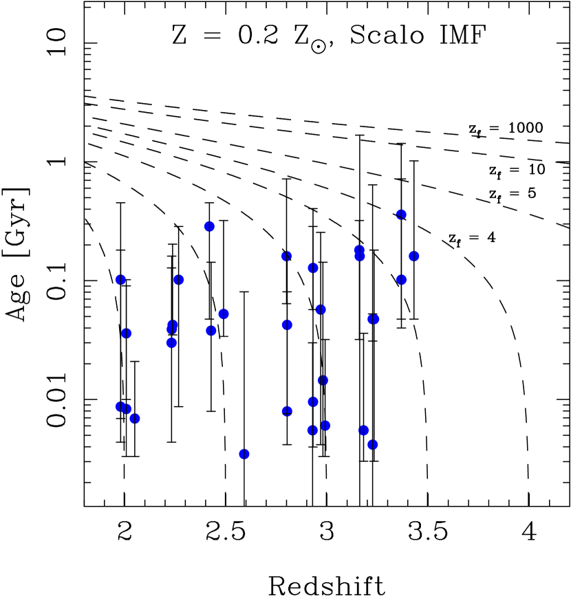
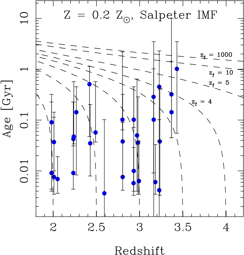
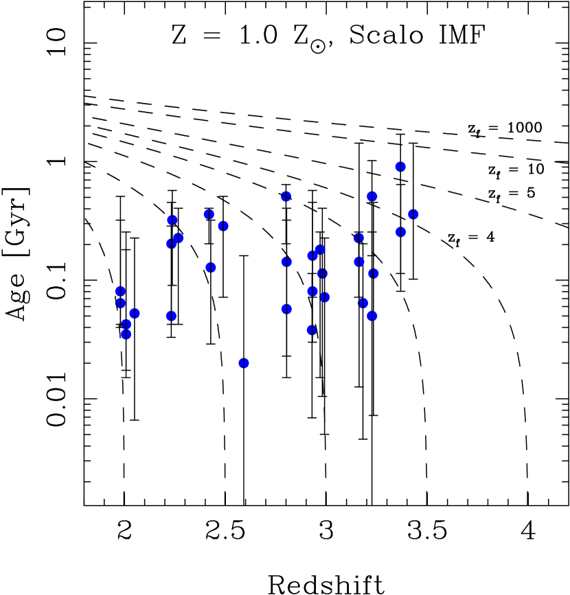
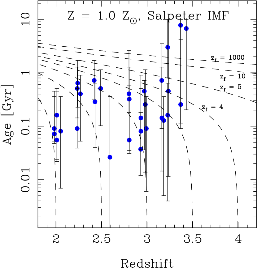
Figure 24: The distribution of LBG stellar population ages as a function of redshift. The data points and error bars show the best–fit ages and their 68% confidence interval from the stellar population synthesis models. The dashed curves show the lookback time from the observed galaxy redshift to constant “formation” redshifts, $z_{f}=2.0$, 2.5, 3.0, 3.5, 4.0, 5.0, 10.0, and 1000 (not all curves are labeled).

Sawicki & Yee (1998) derived upper limits of $t<200$ Myr on the ages of the dominant stellar populations in most HDF LBGs, and concluded that LBGs are dominated by very young populations ($t\sim 25$ Myr). Their models with $\delta$–function star–formation histories have UV luminosities that decline rapidly, mandating young ages for a UV–bright (by definition) LBG population. It is therefore more useful to compare their constant star–formation models to our results. As can been seen from the individual galaxy confidence distributions and the composite age–attenuation plots, many of the LBGs in our sample have allowable models with ages on the order of $t\sim 1$ Gyr. However, it is also true that for the majority of galaxies, our best–fit ages for low metallicity, Salpeter IMF models are also $<200$ Myr, with a weighted mean value of $\sim 70$ Myr, only $\sim 2\times$ the median age found by Sawicki & Yee for $z<3$ galaxies assuming the same metallicity and constant star formation. Adopting more metal rich models or a steeper UV–extinction law shifts the age distribution to larger values, with median or weighted mean values in the range of $100-300$ Myr and a substantial tail extending to $\sim 1$ Gyr or more. Although we generally find somewhat older ages than do Sawicki & Yee, our results do not exclude very young ages of several tens of Myr for many objects, at least not for fits using the low metallicity models.

The ages derived from these best–fit stellar population models are generally much younger than the age of the universe at the LBG redshifts. In Figure 24, we plot the 68% confidence interval on the model ages for each LBG versus the observed galaxy redshift. We also overplot curves showing the lookback times to higher redshifts. The results are somewhat dependent on the particular choices for the IMF and metallicity, and derived ages only apply to the youngest stellar populations under the chosen star–formation histories, which do not necessarily apply to the galaxies as a whole (i.e., the star–formation history for the entire galaxy may indeed be more complex than the simple monotonically decaying models used here). The derived ages from these models generally favor a scenario where most of the galaxies have formed their observed stellar populations (i.e., those stars that dominate the rest–frame UV–to–optical SED) within a rather small redshift interval prior to the redshift at which they are observed, at least for those objects at $z\lesssim 3.0$, where the model age constraints are best. If this is the case, then these LBGs assembled (or, are assembling) their stellar masses relatively rapidly. The LBG sample is devoid of old ($t\gtrsim 1$ Gyr), quiescent galaxies at $2\lesssim z\lesssim 3$, which would be expected to populate the upper–left region of the panels in Figure 24. This might be expected, because the galaxies are selected to be UV–bright, but as we have previously noted, there are few (if any) candidates for old, quiescent galaxies among the NICMOS infrared–selected HDF–N catalog with photometric redshifts $2.0\lesssim z_{\mathrm{ph}}\lesssim 3.5$ (see Figure 1). I.e., there is little evidence for a population of “fading,” post–burst remnants from evolved galaxies formed at $z\gtrsim 3$. However, the presence of older stellar components within the star–forming LBGs, cannot be ruled out. As we will see in §5.2, such older stars could, in principle, provide a significant fraction of the galaxies’ total stellar masses. Under such a scenario, the fitted ages for the young stellar components might not represent the ages of the dominant (by mass) stellar populations.

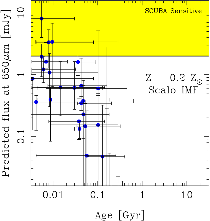
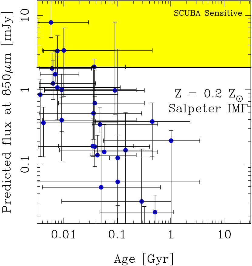
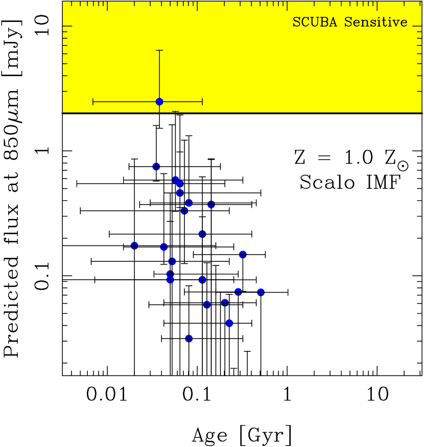
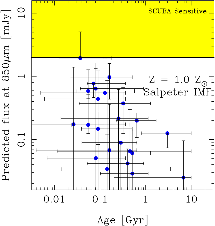
Figure 25: Predicted 850 µm flux densities from the LBGs based on the stellar population and extinction model fitting. The sub–mm fluxes were predicted using the FIR–UV flux density correlation in local starburst galaxies (Meurer et al., 1999; Adelberger & Steidel, 2000), with the dust attenuations derived from the best–fitting models. The four panels correspond to various combinations of IMF and metallicity, as labeled. The yellow shaded region in each panel indicates sensitivity range of the SCUBA 850 µm survey of the HDF–N, $f_{\nu}(850\micron)\gtrsim 2$ mJy (Hughes et al., 1998). For the $0.2$ $Z_{\odot}$ models, one might expect that a few of the youngest, dustiest, and most actively star–forming galaxies could have been detected with SCUBA.

As with extinction, the strong dependence of the derived age distribution on relatively uncertain parameters such as metallicity, the extinction law, and the assumed prior star–formation histories means that one must interpret these results with caution. The question of LBG ages cannot be completely resolved with the available broad–band photometry, and would benefit from a more detailed knowledge and independent data on the chemical enrichment history and dust content of these galaxies, as well as from measurements of starlight at still longer rest–frame wavelengths.

5.1.6 Star Formation Rate

In Table 3, we list the instantaneous star–formation rates for the best–fit models for each LBG. One interesting result is the wide range of SFRs [$10^{-2}\lesssim\Psi/(\hbox{$\mathcal{M}_{\odot}$}\,\mathrm{yr}^{-1})\,\lesssim 10^{3}$] derived for galaxies in the sample, and indeed the wide range even among acceptable models for individual galaxies. The highest derived SFRs mostly correspond to models with young ages (mostly $<15$ Myr) and small $t/\tau$. Most of these are the young, low metallicity, high extinction models discussed above. For ages $\lesssim 10^{7.5}$ yr and small $t/\tau$, the UV luminosity emitted per unit SFR is lower than its asymptotic value at later times because the OB stars that produce most of the UV light are still building up on the main sequence. At later times, their birth and death rates equilibrate, and the UV luminosity per unit SFR stabilizes. This, combined with the large extinction implied for these models, results in model SFRs that are substantially larger than those which would be derived from the UV–luminosity calibrations generally used in the literature (e.g., Madau, Pozzetti & Dickinson, 1998). The large SFRs are required in order to produce the inferred stellar mass on such short timescales. Conversely, a few galaxies can be fit with negligible amounts of ongoing star formation. These are “post–starburst” models with $t\gg\tau$ and ages 90–150 Myr, where the UV light primarily originates from B stars that have not yet left the main sequence.

For the young, low metallicity models with high extinction, the derived instantaneous SFRs are extremely high, ($\mathrm{SFR}\gtrsim 1000$ $\mathcal{M}_{\odot}$ yr^-1). With this combination of high SFRs and extinction, one would expect that most of the energy from star formation should be absorbed by dust and reradiated in the far–infrared, perhaps with significant emission at mid–infrared and radio wavelengths as well. To date, however, there have been no robust detections of LBGs in the HDF–N at mid–IR, far–IR or sub–mm wavelengths (Goldschmidt et al., 1997; Hughes et al., 1998; Downes et al., 1999,  although there are two possible radio detections, Richards 1998). Therefore we can potentially use these surveys to constrain the intrinsic SFRs of these LBGs.

In particular, we considered the SCUBA 850 µm observations of the HDF–N (Hughes et al., 1998), because sub–mm observations are, in principle, quite sensitive to star formation in galaxies from $z\sim 1-10$ due to the strong negative $k$–correction. Using the relations given by Adelberger & Steidel (2000), we predicted LBG flux densities for SCUBA at 850 µm from the observed LBG (rest–frame) UV luminosity and the dust attenuations from the best fit models. Figure 25 shows the predicted 850 µm SCUBA flux density as a function of the LBG stellar population age. For the solar metallicity models, all of the LBGs have predicted 850 µm flux densities that are below (or very close to) the 2 mJy limit of the HDF–N SCUBA observations. For the $Z=0.2$ $Z_{\odot}$ models, however, a few of the galaxies would have predicted 850 µm flux densities $>2$ mJy. In most cases, the predicted sub–mm emission is only slightly above the SCUBA detection threshold. Given the range in the allowable $A_{1700}$ values for each galaxy, the lack of SCUBA detections may not conclusively rule out any particular model. Moreover, recent mm and sub–mm observations of gravitationally lensed high redshift galaxies (van der Werf et al., 2000; Baker et al., 2001) apparently find less far–IR emission than predicted from the far–IR/UV correlations derived at $z=0$. Conversely, Meurer et al. (2000) find that the UV–FIR correlation for local starbursts substantially underpredicts the far–infrared emission from nearby ultraluminous infrared galaxies. At this time, then, it seems difficult to set additional constraints on the SFRs derived from our SED model fitting. Ultimately, if the SFR can be constrained from observations in the FIR, then this could constrain the viable population synthesis models for each LBG.

5.1.7 Stellar Mass

Figures 20 and 22 show the distribution of best–fitting stellar–mass estimates for the spectroscopic LBG sample, under the assumption of the Calzetti and SMC extinction laws, respectively. Recall that due to the simple nature of the star–formation histories of the models, we treat these stellar mass derivations strictly as lower limits; we will consider upper limits to the stellar masses below (§5.2). It is also important to note that this is not a complete sample of galaxies, and certainly not a mass–limited one. The distribution of masses reflects this fact, e.g., in terms of the lower mass limit for the sample.

The (geometric) mean stellar mass of the composite distribution is $\simeq 3(6)\times 10^{9}$ $\mathcal{M}_{\odot}$ for the $Z=0.2$ $Z_{\odot}$ (1.0 $Z_{\odot}$) metallicity and Salpeter IMF models, assuming the starburst extinction relation. Using a Scalo IMF shifts this value to $\simeq 7\times 10^{9}$ $\mathcal{M}_{\odot}$  (insensitive to metallicity). The 68% confidence range of our composite model mass distribution spans the interval $\hbox{$\mathcal{M}$}\sim 10^{9-11}$ $\mathcal{M}_{\odot}$, similar to the range of best–fit values for individual LBGs. The inferred stellar mass would be quite sensitive to the lower mass cutoff of the IMF, a parameter that we do not vary here (see §5.1.1). Thus, our conclusions are based on the assumption that this cutoff does not change from galaxy to galaxy. There is a weak correlation between the stellar mass and the population age for the Salpeter IMF models (no correlation is apparent for either the Scalo or Miller & Scalo IMF models). The distribution of stellar masses for the LBG sample is nearly independent of the assumed dust–extinction law (cf. Figure 20 and Figure 22). We attribute this primarily to the high–quality near–infrared data, which are sensitive to the later–type stars that constitute the bulk of the stellar mass, and where the effects of dust extinction are reduced. The LBG stellar masses are nearly all smaller than those of present–day, $L^{\ast}$ galaxies ($1.4\times 10^{11}h_{70}^{-2}$ $\mathcal{M}_{\odot}$  for a Salpeter IMF, Cole et al. 2001), but are similar to that of the Galactic bulge, $\sim 10^{10}$ $\mathcal{M}_{\odot}$ (Rich, 1999). Sawicki & Yee (1998) estimated similar median masses, $3-8\times 10^{9}$ $\mathcal{M}_{\odot}$, for $Z=0.2$ $Z_{\odot}$, Salpeter IMF models (transforming to our assumed cosmology). In a new, infrared photometric study of a sample of more luminous (mostly $L>L_{UV}^{\ast}$) LBGs, Shapley et al. (2001) derive median stellar masses (for $Z=\hbox{$Z_{\odot}$}$, Salpeter IMF models) that are $\sim 4\times$ larger than those of our fainter HDF objects.

Somerville, Primack, & Faber (2001) have considered various models for the nature and evolution of high redshift galaxies. In particular, they present distributions of stellar ages and masses for “mock–HDF” catalogs derived using their “collisional starburst” model, where high redshift star formation is driven primarily by mergers and tidal interactions. For bright ($\hbox{$V_{606}$}\leq 25.5$) galaxies in the redshift interval $2.0\leq z\leq 3.5$, Somerville et al. predict a broad range of stellar masses, $10^{8}\lesssim\hbox{$\mathcal{M}$}/\hbox{$\mathcal{M}_{\odot}$}\lesssim 10^{11}$, with a median value of $\hbox{$\mathcal{M}$}\approx 8\times 10^{9}$ $\mathcal{M}_{\odot}$ (for $h=0.7$). This is somewhat larger than the mean value (for Salpeter IMF models, as adopted by Somerville et al.) from our small HDF–N sample, but the comparison is not precise because our sample is not complete and magnitude limited at $\hbox{$V_{606}$}\leq 25.5$. The Somerville et al. models include a small tail of objects with masses greater than those of present–day $L^{\ast}$ galaxies, $\hbox{$\mathcal{M}$}\gtrsim 10^{11}$ $\mathcal{M}_{\odot}$, which are not seen in the HDF–N sample. However, this may simply be due to small number statistics of the HDF–N itself. More notably, the collisional starburst model also predicts a significant number of bright ($\hbox{$V_{606}$}\leq 25.5$), low–mass ($10^{8}\lesssim\hbox{$\mathcal{M}$}/\hbox{$\mathcal{M}_{\odot}$}\lesssim 10^{9}$) galaxies, which are also not found in our LBG sample. These are presumably small galaxies that have recently experienced a massive episode of star formation, which pushes them above the optical magnitude limit. They could also be young, dust–free objects, which are also not found in our SED analysis. A comparison with HDF–N LBGs selected from a $V_{606}$–based catalog shows that none with $\hbox{$V_{606}$}\leq 25.5$ are missed in the NICMOS–selected sample. Therefore, given that the colors and fluxes of our spectroscopically selected LBGs are representative of all galaxies with photometric redshifts in this interval in the HDF–N (see Figure 1), the absence of optically bright but low–mass LBGs may point to a discrepancy with the collisional starburst models.

Figure 26: LBG stellar masses versus observed, rest–frame UV luminosity. The different panels show results from exponential star–formation history models with various metallicity and IMF assumptions, and all assuming the Calzetti et al. (2000) starburst extinction law. The points mark the best–fit masses, with error bars indicating the 68% confidence interval. The UV luminosity is given as an absolute magnitude at 1700 Å on the AB scale. The characteristic UV luminosity $\hbox{$L^{\ast}$}_{1700}$ for LBGs at $z\approx 3$ from the luminosity function of Steidel et al. (1999) corresponds to $M^{\ast}_{1700}=-21.0$, marked by a vertical dashed line, while the stellar mass of a present–day $L^{\ast}$ galaxy is indicated by the horizontal dashed line. In each panel, the diagonal dashed line corresponds to a constant mass–to–light ratio $\hbox{$\mathcal{M}$}/L_{\mathrm{UV}}$. The solid lines show a least squares fit of a straight line to the the data.

Figure 27: Same as Figure 26, but using the SMC extinction law.

We find a fairly good correlation between the derived stellar masses and the rest–frame UV luminosity in these galaxies (see Figures 26 and 27). This result is somewhat surprising, because the UV light is generally expected to trace the instantaneous SFR but not necessarily the stellar mass. The scatter of the best–fit values in this correlation is $\sigma(\log\hbox{$\mathcal{M}$}/L_{\mathrm{UV}})\simeq 0.3$ dex, regardless of IMF and metallicity. This correlation could be misleading if the full range of HDF–N galaxies with $2.0\lesssim z_{\mathrm{ph}}\lesssim 3.5$ do not follow this trend. This would require that the low–mass end of the photometric redshift galaxy sample contain a large population of old or highly extincted galaxies, which would produce larger $\hbox{$V_{606}$}-\hbox{$H_{160}$}$ colors at fainter magnitudes. There is no indication of any such population; indeed, if anything the LBG color–magnitude diagram, Figure 1, shows that most of the redder LBGs are brighter. In the next section, we will consider limits on “hidden” stellar mass from previous generations of star formation, and it may be that the apparent $L_{UV}$–mass correlation would be weakened if such mass were indeed present.

The stellar masses of the brighter LBGs, with UV luminosities near the $L^{\ast}$ value from Steidel et al. (1999), are of order $10^{10}$ $\mathcal{M}_{\odot}$. It is interesting to compare this with kinematically estimated masses based on measurements of nebular–emission–line widths for LBGs (see §5.1.5). A naive application of the virial theorem combining these line widths and the typical half–light radii for LBGs suggests masses that are also $\sim 10^{10}$ $\mathcal{M}_{\odot}$. Thus, the stellar masses that we infer for $\sim\hbox{$L^{\ast}$}$ LBGs can account for most or all of the kinematically estimated mass. In fact these stellar–mass estimates are, if anything, lower limits, measuring only the mass of the “young,” actively star forming component of the galaxy. Furthermore, as described in §5.2 below, the total stellar mass could be larger if a maximal old stellar population were present. As Pettini et al. (1998, 2001) have emphasized, the nebular emission lines probably originate in the UV–bright, central regions of the galaxies, and thus may not sample the full gravitational potential well. It is therefore unclear whether these virial estimates really measure the total mass of the LBG dark matter halos. Unless the ratio of dark to luminous matter in LBGs is much smaller than that in present–day galaxies, it appears that the simple virial mass calculations based on the nebular line widths must significantly underestimate the total masses of the dark–matter halos in LBGs.

5.2 Constraints on old stellar populations at $2\lesssim z\lesssim 3.5$

The masses computed from the best–fitting SEDs represent the integrated stellar mass for the stellar population that dominates the rest–frame UV–to–optical light of the galaxy. Strictly speaking, these estimates constitute only a lower limit to the total integrated stellar mass. We may speculate about the existence of older stars in these galaxies that do not substantially contribute to the observed light, but which might contain a significant fraction of the total stellar mass. Observations of star clusters in the Galactic bulge (e.g., McWilliam & Rich 1994, Ortolani et al. 1995) have shown that ages of their stellar populations are consistent with the age of the Universe, implying very early formation epochs (see also Renzini 1999). In principle, a significant mass fraction of old stars could be present in LBGs, but invisible at UV to optical wavelengths, hidden under the glare of younger stars.

In §2 we noted that nearly all infrared–selected HDF–N galaxies with spectroscopic or photometric redshifts in the range $2<z<3.5$ have blue optical–to–infrared colors, suggesting the presence of on–going star formation, and that there were few, if any, candidates for red, non–star–forming, old galaxies at these redshifts. Could old objects with $z\sim 3$ have faded past the NICMOS HDF–N detection limits? For a non–star–forming, passively evolving galaxy at $z=2.7$ with ages of $t=0.5$, 1.0, 2.0, and 2.4 Gyr (the latter being the age of the Universe for the chosen cosmology), and assuming negligible dust extinction, the stellar masses corresponding to the $\hbox{$H_{160}$}=26.5$ limit of the NICMOS HDF–N image are $\hbox{$\mathcal{M}$}\simeq 0.2$, 0.5, 1.0, and $1.3\times 10^{10}$ $\mathcal{M}_{\odot}$, while the corresponding $\hbox{$V_{606}$}-\hbox{$H_{160}$}$ colors are 3.7, 6.1, 7.3, and 7.4 mag, respectively. Many of the LBGs in our sample have derived stellar masses that are greater than these limits. If old objects with comparable mass exist at these redshifts, then they should be detected in the deep, NICMOS data. Similarly, the luminosities of LBGs from our sample at $3\lesssim z\lesssim 3.5$ are large enough that even if their star formation were truncated at the observed epoch, they would still be detectable above the $\hbox{$H_{160}$}<26.5$ limiting magnitude $\sim 1$ Gyr later at $2.0\lesssim z\lesssim 2.5$. While these hypothetical old objects would be too red to meet the LBG selection criteria, we would expect photometric redshift techniques to identify them as high redshift, early–type–galaxy candidates. The “$J$–dropout” HDF-N–JD1 might be such an object, but there are few other examples. In general, there is little difference in the color distribution between the spectroscopically confirmed HDF–N galaxies with $2.0\lesssim z\lesssim 3.5$, and those with photometrically defined redshifts in the same range, and thus we conclude that there are few (if any) massive, old, non–star–forming objects in the HDF–N in this redshift interval.

Although there are few candidates for red, non–star–forming galaxies in this redshift range, there could still, in principle, be a significant mass component of old stars underlying the active star formation in the UV–bright LBGs. The infrared photometry sets an upper limit to the allowable total mass of the combined young and old populations, and the fit to the full UV–to–optical SED sets a maximum mass ratio of old to young stars, or else the observed colors become too red.

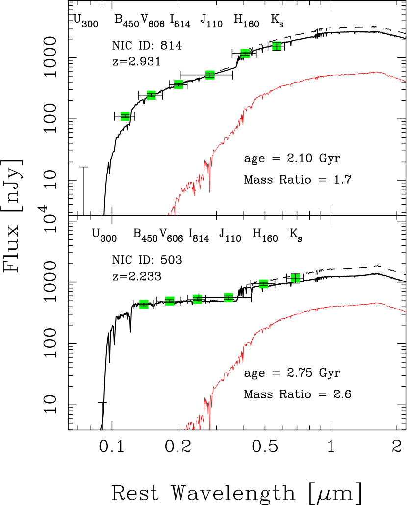
Figure 28: Schematic illustration showing the effect of adding a maximally old stellar population on the best–fitting SEDs of LBGs NIC 503 (HDF 2-903.0) and 814 (HDF 3-93.0). For each object, the data points show the measured photometry with flux uncertainties and bandpass widths indicated by error bars. The solid black line shows the best–fitting “young” model SED for the $Z=0.2$ $Z_{\odot}$ and Salpeter IMF models from Table 3. The red line shows the maximum allowable contribution to the SED from an additional, old stellar population whose age is that of the universe at the galaxy redshift. The mass ratios of the old–to–young stellar populations are given in the panels. The dashed black line shows the superposition of the two components.

To set limits on the LBG mass contribution from old stars, we considered a simple, two–component star–formation–history model. The “young” light from ongoing star formation is represented by the generic suite of models with monotonically decreasing or constant star–formation histories from §4.1 (but restricted here to the Salpeter IMF and metallicities $Z=0.2$ and 1.0 $Z_{\odot}$). We then added a second component to the SED from an old stellar population, formed in a $\delta$–function burst that evolves passively without further star formation. We assumed that this component formed at $z=\infty$, thus maximizing its age ($1.75-3.15$ Gyr for our adopted cosmology) and mass–to–light ratio. The superposition of the two–component SEDs increases the galaxy luminosity predominantly for rest–frame wavelengths, $\lambda_{0}\gtrsim 4000$ Å, as shown for two fiducial LBGs in Figure 28. We then refit each LBG with the full suite of two–component models using the same LBG photometry and uncertainties as in §4. This two component model lets us set an upper limit to the LBG stellar mass, using a stellar population with maximal $M/L$ while still matching the observed UV–to–optical SED.

In order to gauge the fit improvement due to adding a model component from an older stellar population, we applied an $F$–test on the minimum values of $\chi^{2}$ per degree of freedom derived for each galaxy using the two sets of models (the single–component and two–component star–formation histories). For most galaxies, the $F$–test indicates that both models fit the data equally well. However, for a small fraction of the LBG sample, the addition of an old stellar component does improve the goodness–of–fit. Moreover, because the additional model constraint does not significantly degrade the fit to any of the LBGs in the sample, this may actually imply older stellar populations from previous star–formation episodes are indeed present (or at least for some objects). However, based on the limited statistics, it is difficult to assign a significance to this hypothesis. One reasonable conclusion from this test is simply that there is not clear evidence for an absence of old stellar populations underlying the active star formation in LBGs in this sample.

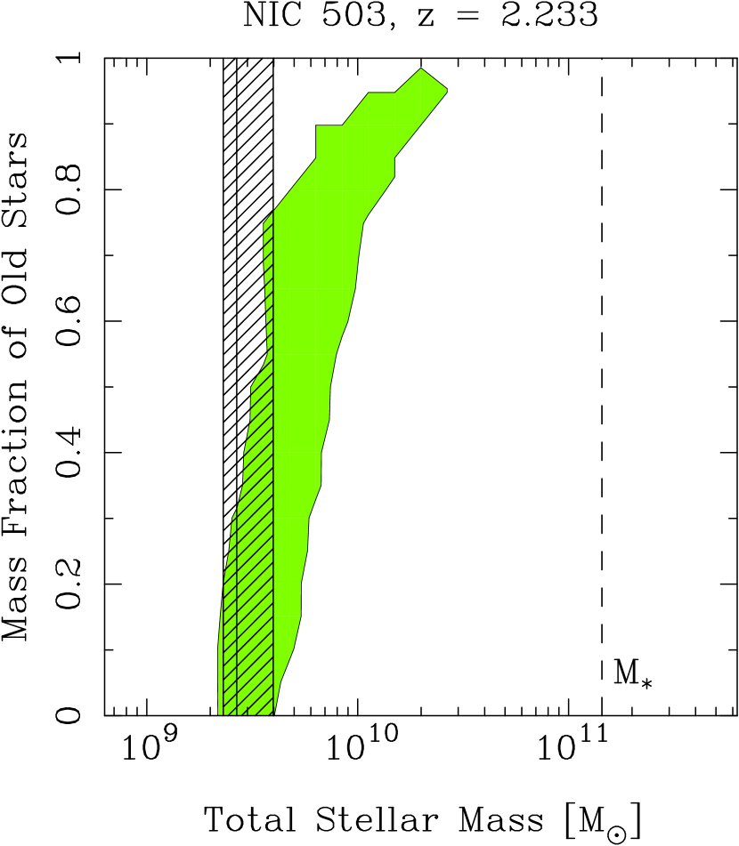
Figure 29: Constraints on the fraction of stellar mass in a hypothetical, old stellar component for two fiducial LBGs. The solid line and the hatched region show the best fitting value and 68% confidence region for the total stellar mass from the single component, “young” models with Salpeter IMF and $Z=0.2$ $Z_{\odot}$. The green shaded region shows the approximate 68% confidence region for the additional stellar mass allowable from a maximally old stellar population, in terms of the mass fraction $\equiv\hbox{$\mathcal{M}$}(\mathrm{Old\;Stars})/[\hbox{$\mathcal{M}$}(\mathrm{Old})+\hbox{$\mathcal{M}$}(\mathrm{Young})]$, as a function of the total stellar mass, $\hbox{$\mathcal{M}$}(\mathrm{Old})+\hbox{$\mathcal{M}$}(\mathrm{Young})$, for best fitting, two component models. The vertical dashed line indicates the mass of a present–day $L^{\ast}$ galaxy.

The two–component models generally favor a slightly different range of parameters than those that best fit the single–age models. The best–fitting ages of the young stellar component from the two–component models are generally somewhat smaller than those derived in §5.1, with correspondingly higher dust extinction. The mean values for the LBG sample are $t\approx 15$ Myr (30 Myr), and $\hbox{$A_{1700}$}\approx 2.4$ mag (1.6 mag) for $Z=0.2$ $Z_{\odot}$ (1.0 $Z_{\odot}$). This is simply a result of the “decomposition” of the observed SEDs into two components, where the “old” component influences the SED only past $\sim 4400$ Å, with only a small amount of recently formed stars in the “young” component, which dominate the UV portion of the SED.

The total stellar masses derived for these two–component models are larger than those from §5.1. This is due to the presence of the older stellar component, which has a large mass–to–light ratio and does not contribute substantially to the light, but do contribute significantly more mass than do the younger stars. Figure 29 shows the relative mass fraction of old stars as a function of the total stellar mass (old + young stars) for the same two fiducial LBGs shown in Figure 28. For these galaxies, and indeed for most of the LBGs, there are viable models where the old stellar populations contain $\gtrsim 90$% of the total stellar mass, while a minority population of young stars dominate the observed SED. However, for most galaxies, the total stellar masses (old and young stars) increase only by factors of a few over the estimates derived using the single–components models. In Figure 30, we compare the best–fitting stellar masses from one– and two–component star–formation history models. On average, the stellar masses from the two–component models are $\approx 3\times$ the masses derived from the single–component models. The (68%) upper mass limits from the two–component models can be $\approx 6-8\times$ the best–fit single–component masses, with these old stars contributing $\lesssim 20$% of the light at rest–frame optical wavelengths. The fraction of mass that can be “hidden” in an older stellar population increases with redshift as the observed bandpasses shift blueward, especially for $z\gtrsim 3$ where the Balmer break shifts through the F160W bandpass. These “maximal $\hbox{$\mathcal{M}$}/L$,” two–component star–formation history models set an upper bound to the total stellar mass, and the results from the one– and two–component models bound the allowable range of LBG stellar masses for a given choice of IMF. Tighter constraints on the total stellar mass will require future observations at still longer rest–frame wavelengths. Deep observations with the SIRTF IRAC instrument will be able to measure the rest–frame $K$–band luminosities of LBGs, at these redshifts, and should provide the best census of LBG stellar mass at these redshifts.

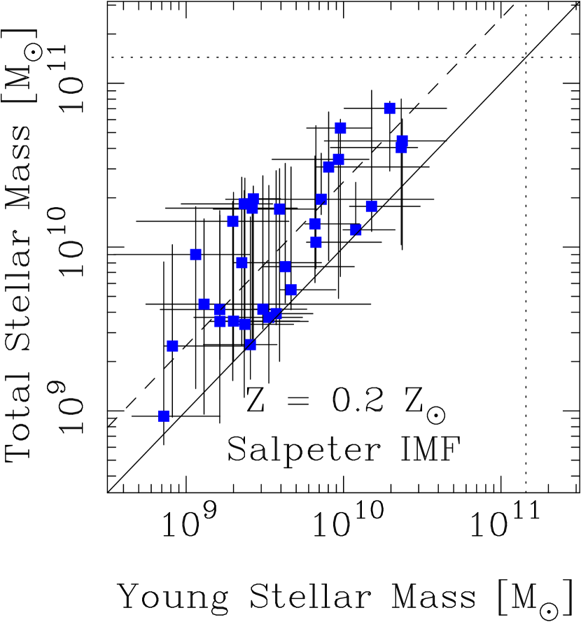
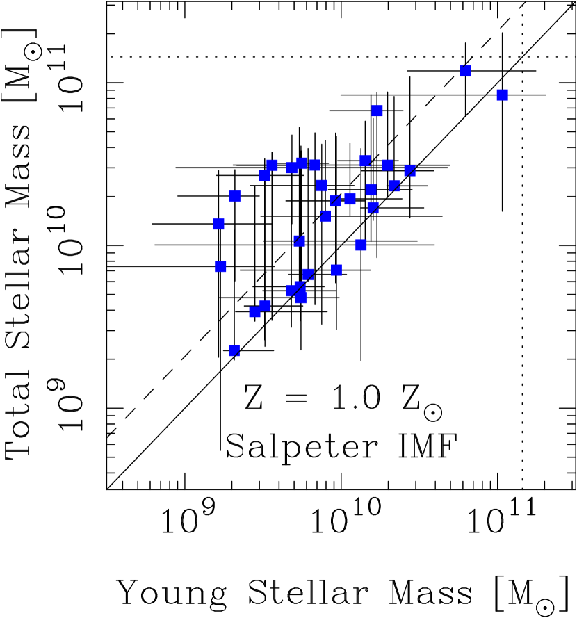
Figure 30: The best–fitting total stellar mass [$\equiv\hbox{$\mathcal{M}$}(\mathrm{Old\;Stars})+\hbox{$\mathcal{M}$}(\mathrm{Young\;Stars})$] for each LBG, plotted against the mass from the single–component models. Each data point shows the range of total stellar mass from the two–component models as a function of the range of stellar masses from the single–component model fits. The error bars correspond to the 68% confidence range on each set of models. The solid line shows a one–to–one mass ratio, while the dashed line indicates the average mass ratio, $X$, of the best–fit values for the LBGs, where $X=(2.9,\;3.1)$ for the $Z=(0.2,\;1.0)$ $Z_{\odot}$ models, respectively. The dotted lines mark the stellar mass of a present–day $L^{\ast}$ galaxy.

5.3 Evolution of Lyman Break Galaxies

The question remains, how do the LBGs fit into the history of galaxy formation and evolution, and what is their fate at $z=0$? As discussed in the introduction, several evolutionary scenarios have been proposed for LBGs. Regardless of the physical parameters that regulate star formation in these objects, these different scenarios predict substantially different end products for their evolution. The clustering observed for LBGs indicates that these galaxies are strongly biased relative to the overall mass distribution in the universe (Giavalisco et al. 1998, Adelberger et al. 1998). This suggests that they are hosted by the most massive dark matter halos at these redshifts, and that they will ultimately become parts of fairly massive galaxies today. In this scenario, the LBGs may plausibly represent the formation stages of the bulges and spheroidal components of massive, present–day galaxies. In contrast, from their analyses of HDF–N LBGs, Sawicki & Yee (1998) concluded that the LBGs will form only a small fraction ($\sim 5$%) of the stellar mass contained in a typical, $L^{\ast}$ galaxy today. That scenario is also consistent with one of the models suggested by Lowenthal et al. (1997), in which the LBGs could be small, sub–galactic clumps that will fade by the present day to represent present–day dwarf elliptical/spheroidal galaxies. This question hinges on our understanding of the fraction of stellar mass that formed has formed at these high redshifts.

By fitting population synthesis models, we have found a range of star–formation histories that adequately match the observed photometry for each galaxy in our sample. If we assume that models were to continue forming stars without change or interruption after the time at which the galaxies are observed, we may predict the subsequent evolution of these galaxies at lower redshifts. For each LBG, we selected all models within the 68% confidence region of the parameter space, i.e., those which best fit the photometric data. Because a range of different models provides acceptable fits to the photometry, there is therefore a wide range of possible end–product masses. Star–formation models with $t\gtrsim\tau$ have already produced the bulk of their stellar populations by the redshift where the galaxy is observed. The colors and luminosities of these models at later times evolve essentially passively, and the stellar masses remain roughly constant, although some of the mass becomes locked up in stellar remnants or is returned to the interstellar medium as stars burn off the main sequence. Alternatively, models with $t\ll\tau$ continue to build stellar mass over their $e$–folding timescale, $\tau$, growing by factors of $\sim\tau/t$ over their lifetimes. For most of the LBG sample, the best–fitting model remains significantly less massive than a present–day $L^{\ast}$ galaxy. However, it is also true that nearly every galaxy has possible models (in the sense that they provide acceptable fits to the observed photometry) that will result in final stellar masses that are greater than those of $L^{\ast}$ galaxies today. Clearly, galaxies cannot continue to form stars continuously at high rates in this fashion for long, because it is unlikely that they have sufficiently large gas reservoirs to fuel such star formation indefinitely.

Although the best–fit stellar masses for nearly all of the HDF–N LBGs are significantly smaller than that of a present–day $L^{\ast}$ galaxy, it is important to remember that most of these galaxies are also fainter than the “typical” $z\approx 3$ LBGs studied in the ground–based survey of Steidel et al.  This can be seen in Figures 26 and 27, where the masses are plotted against the UV luminosities of the galaxies. The characteristic $L^{\ast}$ luminosity at 1700 Å for LBGs from Steidel et al. (1999) is approximately $M_{1700}=-21.0$, which is brighter than most of the HDF–N LBGs. Giavalisco & Dickinson (2001) have found that the fainter HDF–N LBGs cluster less strongly than do their brighter counterparts from the ground–based surveys, suggesting that they are generally associated with less massive dark matter halos. As a result, it might not be surprising if many of them are not in fact destined to become $L>\hbox{$L^{\ast}$}$ galaxies today. The stellar masses plotted in Figures 26 and 27 scale roughly linearly with the UV luminosity, and the intercept at $M_{1700}=-21$ is roughly $10^{10}\hbox{$\mathcal{M}_{\odot}$}$, or $\sim 1/10$th the mass of a present–day $L^{\ast}$ galaxy. As discussed in §5.2, we cannot discount the possibility that LBGs may have a component of older stars from previous episodes of star formation. This could, in principle, significantly boost their stellar masses with little effect on their observed luminosities, but unless all LBGs have the maximum permissible amount of old stellar mass (i.e., unless they actually formed most of their stars at extremely high redshift, $z\gg 3$), then it seems that LBGs with $L^{\ast}$ UV luminosities must generally have smaller stellar masses than their present–day $L^{\ast}$ descendents.

For our adopted cosmology, the co–moving HDF–N volume between $z=2$ and 3.5 is approximately 27000$h_{70}^{-3}$ Mpc³. From the $K$–band luminosity function of Cole et al. (2001), we would expect an average of 23 galaxies with luminosities $L\geq\hbox{$L^{\ast}$}_{K}$ within such a volume in the local universe. Modulo variations due to clustering, their progenitors must be present within this redshift range in the HDF–N, at some earlier stage of evolution – perhaps in many smaller pieces, or even as yet uncollapsed. Of the galaxies that we have analyzed here, only a few have best–fitting star–formation histories that, if extrapolated forward without change to $z=0$, would produce all the stars found in an $L^{\ast}$ galaxy today. There are many other HDF–N LBGs without spectroscopic redshifts (mostly fainter objects, see Figure 1) that we have not analyzed here, and some fraction of these may also grow to comparable masses at $z=0$. In general, then, we can say that the best–fitting stellar population models for HDF–N LBGs have masses smaller than those of $L^{\ast}$ galaxies today, and that most LBGs are likely to remain sub–$L^{\ast}$ without further episodes of star formation (perhaps fueled by gas infall) or substantial merging at lower redshifts. These HDF–N LBGs are less luminous, and thus arguably less massive, than their counterparts from the larger ground–based surveys, and it is unclear whether or not there are enough objects that could “passively” evolve to produce the massive end of the present–day galaxy population without additional star formation or merging. However, these histories are not definitive: for nearly every LBG, there exist allowable models capable of producing (or even overproducing) the total stellar mass of a present–day, $L^{\ast}$ galaxy.

An interesting puzzle results from the fact that the ages of the $2.0<z<2.5$ sub–sample of LBGs are generally much shorter than the span of cosmic time across the redshift range of our entire sample [$t(2<z<3.5)\simeq 1.5$ Gyr]. Because the masses derived for LBGs at $z\sim 3-3.5$ are comparable to those at $z\sim 2-2.5$, we might expect to find a population of old, quiescent galaxies among the many HDF–N objects with (photometrically estimated) redshifts $2.0\lesssim z\lesssim 2.5$. Indeed, given the lifetimes we estimate for the LBG star–formation episodes (with median stellar population ages $t\sim 0.1$ Gyr), such “old” galaxies should outnumber the observed LBGs by a factor of $\sim 1.5\;\mathrm{Gyr}/0.1\;\mathrm{Gyr}=15$. We do not see such a population of old, high–redshift objects, given the narrow range colors observed for galaxies at these redshifts (see Figure 1) to the flux limits of the NICMOS data. Moreover, Steidel et al. (1999) find that the UV luminosity functions of LBGs are indistinguishable (at least for luminosities around $L^{\ast}$) at $z\sim 3$ and $z\sim 4$. The $z\sim 4$ objects must evolve into something, but again there is no evidence for a population of faded remnants at $z<3.5$. Thus the fate of the the $z\sim 3$ LBG population remains somewhat enigmatic.

One possible solution may be found if the simple star–formation prescription (i.e., constant or declining SFR with time) used in our models is incorrect for most objects. Galaxies might maintain a youthful appearance, despite long star–formation timescales, if the SFRs generally increased with time over this redshift range. This, however, may be difficult to reconcile with the apparent lack of evolution in the UV luminosity function between $z=3$ and 4. Alternatively, multiple star–forming episodes with a duty cycle of $t_{d}\lesssim 1$ Gyr might be the norm. In this way, the stars from high redshift LBGs are incorporated into their lower redshift counterparts, with intermittent episodes of star formation to rejuvenate the emergent UV–to–optical spectrum in order to avoid overproducing galaxies with red colors or old SED ages. Interestingly, when we fit LBGs using the two–component models (ongoing star formation plus a maximally–old stellar component, see §5.2), we frequently derive quite small ages for the “young” component (often $t\lesssim 30$ Myr), which may also be an indication that short bursts are the normal mode for star formation at these epochs.

This complex, stochastic evolutionary history is reminiscent of the collisional starburst models of Somerville et al. (2001), although in detail their model appears to predict too broad a range of LBG stellar masses compared to the values we derive. In the general context of hierarchical models for galaxy formation, one might naturally expect that young galaxies are the sites of vigorous merging activity and gas accretion, which can trigger episodic (but frequent) star formation. The total stellar masses resulting from these complex star–formation histories should be bounded at the minimum by the single–component models we have used in this paper, and at the maximum by the two–component models with a maximally old stellar population.

6 Summary

Using WFPC2 ($U_{300}$$B_{450}$$V_{606}$$I_{814}$), NICMOS ($J_{110}$$H_{160}$), and ground–based $K_{s}$–band data, we have investigated the stellar populations of 33 HDF–N LBGs with redshifts $2.0\lesssim z\lesssim 3.5$, reaching the following conclusions:

1. The LBGs have rest–frame UV–to–optical SEDs that are dissimilar to present–day, “Hubble Sequence” spiral and elliptical galaxies, but are comparable to those of local starburst galaxies with modest amounts of dust extinction. Examining complete galaxy samples based on photometric redshifts, we find little evidence for a substantial population of galaxies with redder colors at similar redshifts.

2. By comparing the LBG data in seven broad–bands to stellar population synthesis models, we derive good constraints on the total stellar masses for the LBGs in our sample. The minimum value is derived using single–component star–formation histories, with mean values that range from $3\;(6)\times 10^{9}$ $\mathcal{M}_{\odot}$ for $Z=0.2$ $Z_{\odot}$ (1.0 $Z_{\odot}$) and a Salpeter IMF to $7\times 10^{9}$ $\mathcal{M}_{\odot}$ using a Scalo IMF (for both low and solar metallicity models). For galaxies with $L^{\ast}$ UV luminosities, the inferred masses are $\sim 10^{10}$ $\mathcal{M}_{\odot}$, or roughly 1/10th that of a present–day, $L^{\ast}$ galaxy. Furthermore, we constrain the maximum LBG masses by including a second model component, corresponding to a maximally–old (and hence maximum $M/L$) stellar population hidden in the glare of the ongoing star–formation. We find, on average, that a hypothetical old stellar population could in principle contain up to $\approx 3-8\times$ the stellar mass of the young stars that dominate the observed SED. The stellar masses we derive are comparable to the simple kinematic estimates for LBG masses from nebular–line widths, suggesting that those measurements underestimate the total mass of the LBG dark matter halos. We find a fairly tight correlation between the derived stellar masses and UV luminosity, with a scatter of $\approx 0.3$ dex.

3. The allowable (68% confidence) SED models generally place only loose constraints on the stellar–population ages, dust attenuation, and prior star–formation history. For solar metallicity models, the best–fitting ages for individual galaxies span a range of 30 Myr to $\sim 1$ Gyr, and have dust attenuation factors of $0-3$ mag at 1700 Å. For models with sub–solar metallicity, however, a number of objects are well fit with very young ages ($\lesssim 10$ Myr) and high extinction ($A_{1700}=2.5-4$ mag). The mean ages and extinctions for our LBG sample thus depend somewhat on the particular choice of IMF and metallicity, with ages of 70 Myr (120 Myr) for 0.2 $Z_{\odot}$ (1.0 $Z_{\odot}$) metallicity and Salpeter IMF, and 40 Myr (70 Myr) for 0.2 $Z_{\odot}$ (1.0 $Z_{\odot}$) metallicity and Scalo IMF. The typical dust attenuation correction at 1700 Å is a factor of 4.4 (3.0) for $Z=0.2$ $Z_{\odot}$ (1.0 $Z_{\odot}$), although the total, luminosity weighted mean flux correction for the sample as a whole is larger, 13.8 (4.6), due to larger fitted extinctions for some galaxies with the largest inferred SFRs. These values are consistent with those from Steidel et al. (1999) based on rest–frame UV observations alone of nearly 1000 LBGs. These average correction factors, while possibly applicable to the LBG population as a whole, are probably not very useful for individual galaxies due to the wide allowable range of parameter space for each LBG. We also find that no galaxy in our LBG sample is well fit by young, dust–free, “first–generation” stellar populations. Such objects must be quite rare at these redshifts, or too faint to meet the LBG color selection criteria, or must have SEDs that are significantly different from those produced by the stellar population models we use here.

4. The extrapolated evolution of the best–fit SED models generally indicates that LBGs will remain sub–$L^{\ast}$–sized galaxies today unless they undergo subsequent merging or gas accretion. However, for nearly all the LBGs, there are allowable (68% confidence) models capable of producing the mass of a present–day $L^{\ast}$galaxy, and in some cases many times that of an $L^{\ast}$–galaxy by $z=0$. Based on the derived mass and age distributions, we suggest that star formation at high redshifts may be driven by discrete, recurrent events, which could result from mergers, tidal interactions, etc. These starbursts must occur with a relatively short duty cycle ($\sim 10^{8}\,\mathrm{Gyr}/10^{9}$ Gyr), and a timescale between star–formation events of $t\lesssim 1.5$ Gyr, in order to keep rejuvenating the galaxy SEDs and explain the apparent absence of non–star–forming, evolved, massive galaxies at $z\sim 2$. The LBGs may indeed represent the building sites of massive present–day galaxies, but the dominant stellar–mass assembly may occur via repeating starburst events rather than quiescent, continuous star formation.

Table 1: Observations of the HDF–N.

		$\lambda_{\mathrm{eff}}$	Exposure Time	$m_{\mathrm{lim}}$	PSF
Camera	Bandpass	$(\mu\mathrm{m})$	(ksec)	(AB)	FWHM
WFPC2	F300W	0.30	153.7	27.0	0$\farcs$14
	F450W	0.46	120.6	27.9
	F606W	0.60	109.1	28.2
	F814W	0.80	123.6	27.6
NIC3	F110W	1.10	012.6	26.5	0$\farcs$22
	F160W	1.60	012.6	26.5
KPNO IRIM	$K_{s}$	2.20	082.4	23.8	1″00

Table 2: HDF–N Lyman Break Galaxy Sample

			RA	DEC
NIC ID	WFPC2 ID	$z$	(s)	(mm:ss.s)	$H_{160}$	$V_{606}-H_{160}$	$H_{160}-K_{s}$	Ref.
162	2-585.2	1.980	49.74	14:15.6	24.46	1.10	$<1.02$	5,8
163	2-585.1	1.980	49.82	14:14.8	22.44	1.82	+0.32	5,8
110	2-449.0	2.005	48.30	14:16.6	22.52	1.21	+0.28	1
109	2-454.0	2.009	48.23	14:18.5	23.49	0.97	+0.08	7
1513	3-875.0	2.050	37.07	12.25.3	23.06	0.94	$-0.09$	8
843	3-118.0	2.232	54.71	13:14.8	23.56	0.92	+0.19	6
503	2-903.0	2.233	55.06	13:47.1	23.94	0.70	+0.34	2
274	2-525.0	2.237	50.09	14:01.1	23.58	1.24	+0.51	6
67	2-82.1	2.267	44.07	14:10.1	23.86	0.67	$-0.12$	2
561	2-824.0	2.419	54.61	13:41.4	24.67	0.63	$<-0.73$	2
97	2-239.0	2.427	45.89	14:12.1	23.99	0.75	+0.69	6
741	2-591.2	2.489	53.18	13:22.7	23.99	0.90	+0.29	6
989	4-445.0	2.500	44.64	12:27.4	22.61	1.55	+0.26	3,8
804	4-639.0	2.591	41.72	12:38.8	24.53	0.47	+0.52	1
1352	4-497.0	2.800	45.74	11:57.3	25.11	0.82	+0.32	8
782	4-316.0	2.801	45.02	12:51.1	23.20	1.17	+0.34	8
1357	4-555.1	2.803	45.41	11:53.1	23.21	1.26	+0.28	1
1358	4-555.2	2.803	45.30	11:52.2	23.49	0.85	+0.45	1
522	1-54.0	2.929	44.10	13:10.8	22.96	1.44	+0.36	6
813	4-52.0	2.931	47.72	12:55.8	23.64	1.29	+0.13	2
814	3-93.0	2.931	47.86	12:55.4	23.65	1.70	+0.40	2
1063	4-289.0	2.969	46.94	12:26.1	25.26	0.18	+0.76	6
1541	4-363.0	2.980	48.31	11:45.8	24.51	0.88	+0.56	2
661	2-643.0	2.991	53.42	13:29.4	24.15	0.79	+0.02	2
273	2-76.11	3.160	45.34	13:47.0	25.24	0.24	+1.23	2
367	2-565.0	3.162	51.19	13:48.8	24.15	1.11	$-0.99$	6
282	2-901.0	3.181	53.58	14:10.2	23.97	0.91	$-0.27$	2
1114	4-858.11	3.220	41.17	12:02.9	25.68	0.53	+0.98	1,2,4,8
1115	4-858.0	3.220	41.26	12:03.0	23.89	0.77	+1.00	1,2,4,8
947	3-243.0	3.233	49.80	12:48.8	25.51	0.55	+1.64	2
284	2-834.2	3.367	52.98	14:08.5	26.53	0.65	$<1.41$	8
516	2-637.0	3.368	52.74	13:39.1	24.88	0.54	+0.38	2
553	2-604.0	3.430	52.40	13:37.8	24.43	0.80	+1.16	2

References. — (1) Steidel et al. 1996; (2) Lowenthal et al. 1997; (3) Cohen et al. 1996; (4) Zepf et al. 1997; (5) Elston et al., private communication; (6) Dickinson 1998; (7) Lowenthal, Simard, & Koo 1998; (8) Cohen et al. 2000

Table 3: Best Fit Stellar Population Synthesis Model Parameters

		$Z$		Age	$\tau$	$A_{1700}$	$\log\mathcal{M}$	SFR
NIC ID	$z$	($Z_{\odot}$)	IMF	(Myr)	(Myr)	(mag)	($\mathcal{M}_{\odot}$)	($\mathcal{M}_{\odot}$ yr-1)	$\chi^{2}_{0}$
(1)	(2)	(3)	(4)	(5)	(6)	(7)	(8)	(9)	(10)
162	1.98	0.2	Salpeter	0009.1	00010	3.1	09.0	00068.900	09.2
		1.0	Salpeter	0090.5	00010	0.5	09.4	00000.035	09.2
		0.2	Scalo	0008.7	00010	3.1	09.4	00201.000	09.1
		1.0	Scalo	0080.6	00020	1.0	09.6	00004.120	09.1
163	1.98	0.2	Salpeter	0090.5	00010	2.2	10.5	00000.392	09.5
		1.0	Salpeter	0071.9	00010	2.2	10.4	00002.330	09.7
		0.2	Scalo	0102.0	00030	2.4	10.7	00057.000	09.1
		1.0	Scalo	0064.1	00010	2.2	10.6	00007.560	09.4
110	2.008	0.2	Salpeter	0037.0	02000	3.1	10.1	00345.000	03.3
		1.0	Salpeter	0161.0	02000	2.4	10.3	00148.000	04.2
		0.2	Scalo	0034.0	00050	2.9	10.4	00585.000	03.5
		1.0	Scalo	0035.0	00010	2.2	10.4	00090.000	04.3
109	2.008	0.2	Salpeter	0007.6	00010	3.1	09.4	00217.000	01.2
		1.0	Salpeter	0055.0	00010	1.2	09.8	00002.750	02.5
		0.2	Scalo	0007.9	00030	3.1	09.9	00810.000	01.2
		1.0	Scalo	0042.5	00010	1.4	10.0	00015.100	02.3
1513	2.05	0.2	Salpeter	0006.9	00010	3.1	09.6	00372.000	01.8
		1.0	Salpeter	0080.6	00010	0.5	010.0	00000.333	05.8
		0.2	Scalo	0006.9	00010	3.1	10.0	01067.000	01.7
		1.0	Scalo	0052.5	00010	1.0	10.2	00007.710	05.5
843	2.232	0.2	Salpeter	0009.1	00010	2.9	09.4	00190.000	01.1
		1.0	Salpeter	0090.5	00030	1.2	09.9	00015.200	00.6
		0.2	Scalo	0030.0	00030	2.4	10.0	00217.000	00.9
		1.0	Scalo	0050.0	00010	1.0	10.0	00007.550	00.5
503	2.233	0.2	Salpeter	0042.5	00010	1.2	09.5	00005.310	03.2
		1.0	Salpeter	0509.0	$\infty$	0.7	09.8	00016.400	04.6
		0.2	Scalo	0039.0	00010	1.2	09.8	00013.400	03.9
		1.0	Scalo	0203.0	$\infty$	0.7	09.9	00039.900	06.4
274	2.237	0.2	Salpeter	0047.5	00010	2.2	09.9	00007.600	00.9
		1.0	Salpeter	0641.0	$\infty$	1.7	10.2	00032.100	02.1
		0.2	Scalo	0042.5	00010	2.2	10.2	00020.800	01.6
		1.0	Scalo	0321.0	$\infty$	1.4	10.3	00059.900	04.0
67	2.267	0.2	Salpeter	0143.0	00300	1.2	09.6	00025.300	00.9
		1.0	Salpeter	0404.0	05000	0.7	09.8	00018.900	01.0
		0.2	Scalo	0102.0	02000	1.2	09.8	00064.600	00.7
		1.0	Scalo	0227.0	03000	0.5	09.9	00032.400	00.8
561	2.419	0.2	Salpeter	0509.0	$\infty$	0.5	09.5	00007.310	04.6
		1.0	Salpeter	0719.0	01000	0.0	09.6	00004.590	04.2
		0.2	Scalo	0286.0	03000	0.2	09.5	00011.400	04.7
		1.0	Scalo	0360.0	$\infty$	0.0	09.6	00011.900	05.2
97	2.427	0.2	Salpeter	0035.0	00010	1.4	09.5	00009.050	06.8
		1.0	Salpeter	0286.0	$\infty$	1.0	09.6	00016.900	07.4
		0.2	Scalo	0038.0	00020	1.4	09.7	00045.600	07.2
		1.0	Scalo	0128.0	00200	0.7	09.8	00034.000	07.7
741	2.489	0.2	Salpeter	0057.1	00010	1.4	09.8	00002.160	02.6
		1.0	Salpeter	0509.0	07000	1.4	10.1	00026.300	02.6
		0.2	Scalo	0052.5	00010	1.4	10.0	00005.540	02.7
		1.0	Scalo	0286.0	00700	1.0	10.1	00034.400	03.0
989	2.5	0.2	Salpeter	0002.5	00010	5.8	10.8	23043.000	07.9
		1.0	Salpeter	0004.8	00020	5.1	10.3	03918.000	08.1
		0.2	Scalo	0002.6	00010	5.3	11.1	42544.000	09.6
		1.0	Scalo	0004.2	00010	5.1	10.8	12250.000	08.6
804	2.591	0.2	Salpeter	0003.6	00020	2.9	09.3	00505.000	02.5
		1.0	Salpeter	0026.3	00010	1.4	09.3	00017.500	01.4
		0.2	Scalo	0003.5	02000	2.9	09.8	01795.000	02.6
		1.0	Scalo	0020.0	00010	1.4	09.6	00057.800	01.5
1352	2.8	0.2	Salpeter	0102.0	00010	0.0	09.3	00000.009	06.0
		1.0	Salpeter	0404.0	00200	0.0	09.5	00003.080	05.2
		0.2	Scalo	0161.0	00050	0.0	09.5	00002.770	06.1
		1.0	Scalo	0509.0	03000	0.0	09.7	00008.460	05.5
782	2.801	0.2	Salpeter	0001.0	00010	5.1	10.6	32518.000	13.8
		1.0	Salpeter	0001.0	00010	5.1	10.4	23486.000	16.8
		0.2	Scalo	0002.5	00010	4.8	10.9	29417.000	14.3
		1.0	Scalo	0001.0	00010	4.8	10.8	56860.000	16.8
1357	2.803	0.2	Salpeter	0007.6	00010	3.6	09.9	00745.000	00.4
		1.0	Salpeter	0055.0	00010	1.7	10.3	00009.480	00.6
		0.2	Scalo	0007.9	00020	3.6	10.4	02588.000	00.5
		1.0	Scalo	0057.1	00020	1.9	10.6	00114.000	00.5
1358	2.803	0.2	Salpeter	0038.0	00010	1.9	10.1	00029.700	01.5
		1.0	Salpeter	0321.0	07000	1.4	10.3	00072.100	02.1
		0.2	Scalo	0042.5	00020	1.9	10.3	00156.000	02.1
		1.0	Scalo	0143.0	07000	1.4	10.3	00162.000	02.9
522	2.929	0.2	Salpeter	0005.8	00200	4.3	10.3	03095.000	01.5
		1.0	Salpeter	0037.0	00010	2.9	10.5	00094.400	02.1
		0.2	Scalo	0005.5	00500	4.3	10.7	09661.000	01.5
		1.0	Scalo	0038.0	00030	3.1	10.8	00806.000	02.0
813	2.931	0.2	Salpeter	0102.0	00010	1.0	10.2	00000.062	03.0
		1.0	Salpeter	0143.0	00010	0.0	10.2	00000.001	01.1
		0.2	Scalo	0128.0	00010	0.5	10.3	00000.006	02.5
		1.0	Scalo	0161.0	00030	0.0	10.3	00003.110	01.3
814	2.931	0.2	Salpeter	0010.0	00010	4.3	10.0	00569.000	01.0
		1.0	Salpeter	0080.6	00010	1.9	10.4	00000.882	00.2
		0.2	Scalo	0009.5	00010	4.3	10.4	01565.000	00.9
		1.0	Scalo	0080.6	00020	2.2	10.6	00036.100	00.2
1063	2.969	0.2	Salpeter	0050.0	00020	0.7	09.2	00007.260	01.1
		1.0	Salpeter	0453.0	10000	0.0	09.4	00006.980	01.1
		0.2	Scalo	0040.0	00020	0.7	09.4	00020.500	01.1
		1.0	Scalo	0181.0	$\infty$	0.0	09.4	00015.500	01.2
1541	2.98	0.2	Salpeter	0036.0	00020	2.4	09.7	00044.900	00.3
		1.0	Salpeter	0255.0	10000	1.7	09.9	00033.200	00.3
		0.2	Scalo	0014.5	00010	2.7	09.9	00190.000	00.4
		1.0	Scalo	0114.0	07000	1.7	10.0	00085.900	00.4
661	2.991	0.2	Salpeter	0005.8	00010	2.9	09.5	00367.000	01.2
		1.0	Salpeter	0080.6	00070	1.7	09.8	00049.600	01.6
		0.2	Scalo	0006.0	00030	2.9	09.9	01247.000	01.2
		1.0	Scalo	0071.9	00700	1.7	10.1	00163.000	01.6
273	3.16	0.2	Salpeter	0286.0	10000	0.5	09.4	00008.670	06.6
		1.0	Salpeter	0641.0	07000	0.0	09.6	00006.560	06.1
		0.2	Scalo	0143.0	00200	0.2	09.5	00014.700	06.8
		1.0	Scalo	0227.0	$\infty$	0.0	09.6	00014.200	06.8
367	3.162	0.2	Salpeter	0090.5	00010	1.0	010.0	00000.118	10.5
		1.0	Salpeter	0114.0	00020	0.5	09.9	00001.580	10.4
		0.2	Scalo	0128.0	00010	0.2	10.1	00000.004	10.0
		1.0	Scalo	0090.5	00010	0.2	10.1	00000.141	10.1
282	3.181	0.2	Salpeter	0005.8	00030	3.1	09.7	00705.000	04.7
		1.0	Salpeter	0128.0	01000	1.9	10.1	00094.100	05.2
		0.2	Scalo	0005.5	00100	3.1	10.2	02340.000	04.7
		1.0	Scalo	0064.1	00500	1.9	10.3	00255.000	05.2
1114	3.226	0.2	Salpeter	0004.2	00010	2.7	09.0	00174.000	03.9
		1.0	Salpeter	0161.0	05000	1.2	09.3	00015.300	04.1
		0.2	Scalo	0004.0	00010	2.7	09.4	00542.000	04.0
		1.0	Scalo	0050.0	$\infty$	1.4	09.4	00056.300	04.2
1115	3.226	0.2	Salpeter	0453.0	$\infty$	1.4	10.4	00063.400	08.2
		1.0	Salpeter	3000.0	$\infty$	0.7	10.9	00032.500	05.5
		0.2	Scalo	0047.5	00010	1.4	10.4	00021.100	08.7
		1.0	Scalo	0509.0	07000	0.5	10.5	00064.500	09.1
947	3.233	0.2	Salpeter	0036.0	00010	1.7	09.5	00009.440	20.8
		1.0	Salpeter	0453.0	07000	1.0	09.8	00016.200	20.9
		0.2	Scalo	0045.0	00300	1.9	09.7	00111.000	21.2
		1.0	Scalo	0090.5	00200	1.2	09.7	00051.300	21.3
284	3.367	0.2	Scalo	0360.0	00200	0.0	09.3	00001.900	01.3
		1.0	Salpeter	6000.0	$\infty$	0.5	10.1	00002.240	02.0
		0.2	Salpeter	0321.0	00100	0.0	09.2	00000.685	01.2
		1.0	Scalo	0905.0	$\infty$	0.0	09.5	00003.350	02.2
516	3.368	0.2	Salpeter	0143.0	00030	0.0	09.7	00001.820	00.7
		1.0	Salpeter	0255.0	00100	0.0	09.8	00006.990	00.6
		0.2	Scalo	0102.0	00020	0.0	09.9	00002.450	00.7
		1.0	Scalo	0255.0	00200	0.0	10.0	00019.600	00.6
553	3.43	0.2	Salpeter	1020.0	$\infty$	1.2	10.5	00031.200	06.5
		1.0	Salpeter	6500.0	$\infty$	0.7	11.1	00022.300	05.4
		0.2	Scalo	0161.0	00030	0.0	10.2	00002.290	06.8
		1.0	Scalo	0360.0	00200	0.0	10.3	00020.000	06.4

References

- Adelberger et al. (1998) Adelberger, K. L., Steidel, C. C., Giavalisco, M., Dickinson, M., Pettini, M., & Kellogg, M. 1998, ApJ, 505, 18
- Adelberger & Steidel (2000) Adelberger, K. L., & Steidel, C. C. 2000, ApJ, 544, 218
- Baker et al. (2001) Baker, A. J., Lutz, D., Genzel, R., Tacconi, L. J., & Lehnert, M. D. 2001, A&A, in press (missingastro-ph/0104345)
- Baugh et al. (1998) Baugh, C. M., Cole, S., Frenk, C. S., & Lacey, C. G. 1998, ApJ, 498, 504
- Bertin & Arnouts (1996) Bertin, E., & Arnouts, S. 1996, A&AS, 117, 393
- Brandt et al. (2001) Brandt, W. M., et al. 2001, AJ, in press (missingastro-ph/0102411)
- Brinchmann & Ellis (2000) Brinchmann, J., & Ellis, R. S. 2000, ApJ, 536, L77
- Bruzual & Charlot (1993) Bruzual, G. A., & Charlot, S. 1993, ApJ, 405, 538
- Bruzual (2000) Bruzual, G. A. 2000, in Proceedings of the XI Canary Islands Winter School of Astrophysics on Galaxies at High Redshift, eds. I. Perez-Fournon, M. Balcells, & F. Sanchez, in press (missingastro-ph/0011094)
- Budavári et al. (2000) Budavári, T., Szalay, A. S., Connolly, A. J., Csabai, I., & Dickinson, M. 2000, AJ, 120, 1588
- Calzetti et al. (1994) Calzetti, D., Kinney, A. L., & Storchi–Bergmann, T. 1994, ApJ, 429, 582
- Calzetti (1997) Calzetti, D. 1997, in The Ultraviolet Universe at Low and High Redshift, eds. W. H. Waller et al. (New York: AIP), 403
- Calzetti et al. (2000) Calzetti, D., Armus, L., Bohlin, R. C., Kinney, A. L., Koornneef, J., & Storchi–Bergmann, R. 2000, ApJ, 533, 682
- Charlot et al. (1996) Charlot, S., Worthey, G., & Bressan, A. 1996, ApJ, 457, 625
- Cohen et al. (1996) Cohen, J. G., Cowie, L. L., Hogg, D. W., Songaila, A., Blandford, R., Hu, E. M., & Shopbell, P. 1996, ApJ, 471, L5
- Cohen et al. (2000) Cohen, J. G., Hogg, D., Blandford, R., Cowie, L., Hu, E., Songaila, A., Shopbell, P., & Richberg, K. 2000, ApJ, 538, 29
- Cohen (2001) Cohen, J. G. 2001, AJ, in press (missingastro-ph/0101251)
- Cole et al. (2001) Cole, S., et al. 2001, MNRAS, in press (missingastro-ph/0012429)
- Coleman et al. (1980) Coleman, G. D., Wu, C.-C., & Weedman, D. W. 1980, ApJS, 43, 393 (CWW)
- Cowie et al. (1996) Cowie, L. L., Songaila, A., Hu, E. M., & Cohen, J. G. 1996, AJ, 112, 839
- Daddi, Cimatti, & Renzini (2000) Daddi, E., Cimatti, A., & Renzini, A. 2000, A&A, 362, L45
- Dickinson (1995) Dickinson, M. 1995, in Fresh Views of Elliptical Galaxies, eds. A. Buzzoni, A. Renzini, & A. Serrano (San Francisco: ASP), 283
- Dickinson (1998) Dickinson, M. 1998, in The Hubble Deep Field, eds. M. Livio, S. M. Fall, & P. Madau (Cambridge, Cambridge Univ. Press), 219
- Dickinson (1999) Dickinson, M. 1999, in After the Dark Ages: When Galaxies were Young, eds. S. Holt & E. Smith, AIP, 122
- Dickinson (2000) Dickinson, M. 2000, Phil. Trans. R. Soc. Lond. A, 358, 2001
- Dickinson et al. (2000) Dickinson, M. et al. 2000, ApJ, 531, 624
- Dickinson et al. (2001) Dickinson, M. et al. 2001, in preparation
- Downes et al. (1999) Downes, D. et al. 1999, A&A, 347, 809
- Dunlop et al. (1996) Dunlop, J., Peacock, J., Spinrad, H., Dey, A., Jimenez, R., Stern, D., & Windhorst, R. 1996, Nature, 381, 581
- Eales et al. (1993) Eales, S., Rawlings, S., Puxley, P., Rocca–Volmerange, B., & Kuntz, K. 1993, Nature, 363, 6425
- Eisenhardt & Dickinson (1992) Eisenhardt, P., & Dickinson, M. 1992, ApJ, 399, L47
- Fernández–Soto, Lanzetta, & Yahil (1999) Fernández–Soto, A., Lanzetta, K. M., & Yahil, A. 1999, ApJ, 513, 34
- Fernández–Soto et al. (2001) Fernández–Soto, A., Lanzetta, K. M., Chen, H. –W., Pascarelle, S., & Yahata, N. 2001, ApJS, in press (missingastro-ph/0007447)
- Folkes et al. (1999) Folkes, S., et al. 1999, MNRAS, 308, 459
- Giavalisco, Steidel, & Macchetto (1996) Giavalisco, M., Steidel, C. C., & Macchetto, F. D. 1996, ApJ, 470, 189
- Giavalisco et al. (1998) Giavalisco, M., Steidel, C. C., Adelberger, K. L., Dickinson, M., Pettini, M., & Kellogg, M. 1998, ApJ, 503, 543
- Giavalisco & Dickinson (2001) Giavalisco, M., & Dickinson, M. 2001 ApJ, 550, 177
- Goldschmidt et al. (1997) Goldschmidt, P. et al. 1997, MNRAS, 289, 465
- Governato et al. (1998) Governato, F., Baugh, C. M., Frenk, C. S., Cole, S., Lacey, C. G., Quinn, T., & Stadel, J. 1998, Nature, 392, 359
- Guhathakurta et al. (1990) Guhathakurta, P., Tyson, J. A., & Majewski, S. R. 1990, ApJ, 357, L9
- Hornschemeier et al. (2000) Hornschemeier, A. E., et al. 2000, ApJ, 541, 49
- Hughes et al. (1998) Hughes, D., et al. 1998, Nature, 394, 241
- Kauffman & Charlot (1998) Kauffman, G., & Charlot, S. 1998, MNRAS, 297, L23
- Kinney et al. (1996) Kinney, A. L., Calzetti, D., Bohlin, R. C., McQuade, K., Storchi-Bergmann, T., & Schmitt, H. R. 1996, ApJ, 467, 38
- Leitherer et al. (2001) Leitherer, C., Leao, J., Heckman, T., Lennon, D., Pettini, M., & Robert, C. 2001, ApJ, in press (missingastro-ph/0012358)
- Lejeune, Cuisinier, & Buser (1997) Lejeune, T., Cuisinier, F., & Buser, R. 1997, A&AS, 125, 229
- Lowenthal et al. (1997) Lowenthal, J. D., et al. 1997, ApJ, 481, 673
- Lowenthal et al. (1998) Lowenthal, J. D., Simard, L., & Koo, D.C. 1998, in The Young Universe: Galaxy Formation and Evolution at High Redshift, eds. S. D’Odorico, A. Fontana & E. Giallongo, (San Francisco, ASP), 110
- Madau (1995) Madau, P. 1995, ApJ, 441, 18
- Madau, Pozzetti & Dickinson (1998) Madau, P., Pozzetti, L., & Dickinson, M. 1998, ApJ, 498, 106
- McWilliam & Rich (1994) McWilliam, A., & Rich, R. M. 1994, ApJS, 91, 749
- Meurer et al. (1997) Meurer, G. R., Heckman, T. M., Lehnert, M. D., Leitherer, C., & Lowenthal, J. 1997 AJ, 114, 54
- Meurer et al. (1999) Meurer, G. R., Heckman, T. M., & Calzetti, D. 1999 ApJ, 521, 64
- Meurer et al. (2000) Meurer, G. R., Heckman, T. M., Seibert, M., Goldader, J., Calzetti, D., Sanders, D., & Steidel, C. C. 2000, in Cold Gas and Dust at High Redshift, ed. D. Wilner, (ASP: San Francisco), in press (missingastro-ph/0011201)
- Miller & Scalo (1979) Miller, G. E., & Scalo, J. M. 1979, ApJS, 41, 513
- Moorwood et al. (2000) Moorwoord, A. F. M., van der Werf, P. P., Cuby, J. G., & Oliva, E. 2000, A&A, 362, 9
- Ortolani et al. (1995) Ortolani, S., Renzini, A., Gilmozzi, R., Marconi, G., Barbuy, B., Bica, E., Rich, R. M. 1995, Nature, 377, 701
- Papovich & Dickinson (2001) Papovich, C., & Dickinson, M. 2001, in preparation
- Pei (1992) Pei, Y. C. 1992, ApJ, 395, 130
- Pettini et al. (1997) Pettini, M., Smith, L. J., King, D. L., & Hunstead, R. W. 1997, ApJ, 486, 665
- Pettini et al. (1998) Pettini, M., Kellogg, M., Steidel, C. C., Dickinson, M., Adelberger, K. L., & Giavalisco, M. 1998, ApJ, 508, 539
- Pettini et al. (2000) Pettini, M., Steidel, C. C., Adelberger, K. L., Dickinson, M., & Giavalisco, M. 2000, ApJ, 528, 96
- Pettini (2000) Pettini, M. 2000, Phil. Trans. R. Soc. Lond. A, 358, 2035
- Pettini et al. (2001) Pettini, M., Shapley, A. E., Steidel, C. C., Cuby, J.–G., Dickinson, M., Moorwood, A. F. M., Adelberger, K. L., & Giavalisco, M. 2001, ApJ, in press (missingastro-ph/0102456)
- Pickles (1998) Pickles, A. J. 1998, PASP, 110, 863
- Renzini (1999) Renzini, A. 1999, in The Formation of Galactic Bulges, eds. C. M. Carollo, H. C. Ferguson, & R. F. G. Wyse, (Cambridge, Cambridge Univ. Press), 9
- Rich (1999) Rich, R. M. 1999, in The Formation of Galactic Bulges, eds. C. M. Carollo, H. C. Ferguson, & R. F. G. Wyse, (Cambridge, Cambridge Univ. Press), 54
- Rich & McWilliam (2000) Rich, R. M., & McWilliam, A. 2000, in Discoveries and Research Prospects from 8–10-Meter-Class Telescopes, Proceedings of the SPIE vol. 4005, ed. J. Bergeron, 150
- Richards et al. (1998) Richards, E. A., Kellermann, K. I., Folmalont, E. B., Windhorst, R. A., & Partridge, R. B. 1998, AJ, 116, 1039
- Salpeter (1955) Salpeter, E. E. 1955, ApJ, 121, 161
- Stanford, Eisenhardt, & Dickinson (1998) Stanford, S. A., Eisenhardt, P. R., & Dickinson, M. 1998, ApJ, 492, 461
- Sawicki & Yee (1998) Sawicki, M., & Yee, H. K. C. 1998, ApJ, 115, 1329
- Scalo (1986) Scalo, J. M. 1986, Fundamentals of Cosmic Physics, 11, 1
- Shapley et al. (2001) Shapley, A. E., Steidel, C. C., Adelberger, K. L., Dickinson, M., Giavalisco, M., & Pettini, M. 2001, ApJ, submitted
- Somerville et al. (2001) Somerville, R. S., Primack, J. R., & Faber, S. M. 2001, MNRAS, 320, 504
- Songalia et al. (1990) Songalia, A., Cowie, L. L., & Lilly, S. J. 1990, ApJ, 348, 371
- Steidel & Hamilton (1992) Steidel, C. C., & Hamilton, D. 1992, AJ, 104, 941
- Steidel, Pettini, & Hamilton (1995) Steidel, C. C., Pettini, M., & Hamilton, D. 1995, AJ, 110, 2519
- Steidel et al. (1996a) Steidel, C. C., Giavalisco, M., Dickinson, M., & Adelberger, K. L. 1996a, AJ, 112, 352
- Steidel et al. (1996b) Steidel, C. C., Giavalisco, M., Pettini, M., Dickinson, M., & Adelberger, K. L. 1996b, ApJ, 462, L17
- Steidel et al. (1999) Steidel, C. C., Adelberger, K. L., Giavalisco, M., Dickinson, M., & Pettini, M. 1999, ApJ, 519, 1
- Teplitz et al. (2000a) Teplitz, H. I., et al. 2000, ApJ, 533, L65
- Teplitz et al. (2000b) Teplitz, H. I., et al. 2000, ApJ, 542, 18
- Thompson et al. (1998) Thompson, R. I., Rieke, M., Schneider, G., Hines, D. C., & Corbin, M. R. 1998, ApJ, 492, L95
- van der Werf et al. (2000) van der Werf, P., Knudsen, K., Labbé, I., & Franx, M. 2000, in Deep Millimeter Surveys, eds. J. Lowenthal & D. Hughes, World Scientific, in press (missingastro-ph/0010459)
- Warren et al. (1987) Warren, S. J., Hewitt, P. C., Irwin, M. J., McMahon, R. G., Bridgeland, M. T., Bunclark, P. S., & Kibblewhite, E. J. 1987, Nature, 325, 131
- Williams et al. (1996) Williams, R. E., et al. 1996, AJ, 112, 1335
- Zepf, Moustakas, & Davis (1997) Zepf, S. E., Moustakas, L. A., & Davis, M. 1997, ApJ, 474, L1