Stellar models in IR calibration

Abstract

For the astronomical community analyzing ISO-SWS data, a first point to assess when judging and qualifying the observational data concerns the flux calibration accuracy. Since the calibration process is not straightforward and since a wrong calibration may lead to an over- or underestimation of the results, knowledge on the full calibration process and on the still remaining calibration problems is crucial when processing the data.

One way to detect calibration problems is by comparing observed data with theoretical predictions of a whole sample of calibration sources. By using an iterative process in which improvements on both the calibration and the theoretical modelling are involved, we will demonstrate that a consistent theoretical data-set of infrared spectra has been constructed. This data-set has been used to derive the OLP10 flux calibration of the ISO-SWS. We will shown that the relative flux calibration accuracy of (high-flux) ISO-SWS observations has reached a 2 % level of accuracy in band 1 and that the flux calibration accuracy in band 2 has improved significantly with the introduction of the memory-effect corrrection and the use of our synthetic spectra for the flux calibration derivation, reaching a 6 % level of accuracy in band 2.

1 INTRODUCTION: SCIENTIFIC GOALS

The modelling and interpretation of the ISO-SWS data requires an accurate calibration of the spectrometers ([Shipman2001]). For this purpose, many calibration sources are observed. In the SWS spectral region (2.38 – 45.2 $\mu$m) the primary standard calibration candles are bright, mostly cool, stars. The better the behaviour of these calibration sources in the infrared is known, the more accurate the spectrometers will be calibrated. ISO however offered the astronomical community the first opportunity to perform spectroscopic observations between 2.38 and 45.2 $\mu$m at a spectral resolving power of $\sim 1500$, not polluted by any molecular absorption caused by the earth’s atmosphere. Consequently the theoretical predictions for these sources are not perfect due to errors in the computation of the stellar models or in the generation of the synthetic spectra or due to the restriction of our knowledge on the mid-infrared behaviour of these sources. A full exploitation of the ISO-SWS data can therefore only result from an iterative process in which both new theoretical developments on the computation of the stellar spectra and more accurate instrumental calibration are involved. Till now, the detailed spectroscopic analysis of the ISO-SWS data in the framework of this iterative process has been restricted to the wavelength region from 2.38 to 12 $\mu$m. So, if not specified, the wavelength range under research is limited to band 1 (2.38 – 4.08 $\mu$m) and band 2 (4.08 – 12.00 $\mu$m).

This paper is organized as follows: in Sect. 2 the method of analysis will be shortly described. An overview of the main results will be given in Sect. 3, while the impact on the calibration of the SWS spectrometers will be elaborated on in Sect. 4. The resultant set of 16 IR synthetic spectra will be compared with the SEDs by Cohen ([Cohen et al.1992], [Cohen et al.1995], [Cohen et al.1996], [Witteborn et al.1999]) in Sect. 5 and in the last section, Sect. 6 we will end with some lessons learned from ISO for future instruments.

2 METHOD OF ANALYSIS

Precisely because this research involves an iterative process, one has to be extremely careful not to confuse technical detector problems with astrophysical issues. Therefore several precautions are taken and the analysis in its entirety enclosed several steps including 1. a spectral cover of standard infrared sources from A0 to M8, 2. a homogeneous way of data reduction, 3. a detailed literature study, 4. a detailed knowledge of the impact of the various stellar parameters on the spectral signature, 5. a statistical method to test the goodness-of-fit (Kolmogorov-Smirnov test) and 6. high-resolution observations with two independent instruments. All of these steps are elaborated on in [*]LD_decin2000 and [*]LD_decin2001_II.

3 RESULTS

Using this method, all hot stars in our sample (i. e. stars whose effective temperature is higher than the effective temperature of the Sun) and cool stars are analyzed carefully. Computing for the first time synthetic spectra in the infrared by using the MARCS-code ([*]LD_gustafsson1975 and subsequent updates) is one step, distilling useful information from it is a second — and far more difficult — one. Fundamental stellar parameters for the sample of calibration sources are a first direct result. In papers III and IV in the series ‘ISO-SWS calibration and the accurate modelling of cool-star atmospheres’ ([Decin et al.2001b] and [Decin et al.2001c]) these parameters are discussed and confronted with other published stellar parameters.

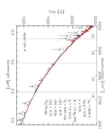
Figure 1: Comparison between the ISO-SWS data of $\alpha$ Cen A (black) and the synthetic spectrum (red) with stellar parameters T_eff = 5830 K, $\log$ g = 4.35, M = 1.3 M_⊙, z = 0.25, $\xi_{t}$ = 1.0 $\rm{km\,s^{-1}}$, $\mathrm{{}^{12}C/^{13}C}$ = 89, $\varepsilon$(C) = 8.74, $\varepsilon$(N) = 8.26, $\varepsilon$(O) = 9.13 and $\theta_{d}$ = 8.80 mas. Some of the most prominent discrepancies between these two spectra are indicated by an arrow.

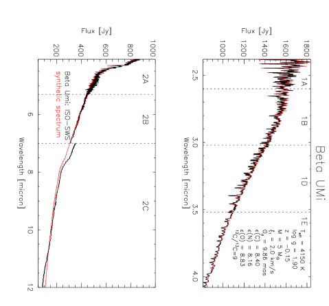
Figure 2: Comparison between band 1 and band 2 of the ISO-SWS data of $\beta$ UMi (black) and the synthetic spectrum (red) with stellar parameters T_eff = 4150 K, $\log$ g = 1.90, M = 5 M_⊙, z = $-0.15$, $\xi_{t}$ = 2.0 $\rm{km\,s^{-1}}$, $\mathrm{{}^{12}C/^{13}C}$ = 9, $\varepsilon$(C) = 8.40, $\varepsilon$(N) = 8.16, $\varepsilon$(O) = 8.83 and $\theta_{d}$ = 9.86 mas.

Far more interesting are however the discrepancies which emerge from the confrontation between ISO-SWS (OLP8.4) and theoretical spectra. A typical example of both a hot and cool star is depicted in Fig. 1 and Fig. 2 respectively. By scrutinizing carefully the various discrepancies between the ISO-SWS data and the synthetic spectra of the standard stars in our sample, the origin of the different discrepancies was elucidated. A description of the general trends in discrepancies for both hot and cool stars can be found in [*]LD_decin2001_II, while the hot stars are discussed individually in [*]LD_decin2001_III and the cool stars in [*]LD_decin2001_IV. A summary of the different kinds of discrepancies and the reason why they arise is given in Table 1.

Table 1: Summary of the origins of the different types of discrepancies found between the ISO-SWS data and the synthetic spectra for the standard calibration sources in our sample.

HOT stars	COOL stars
1. hydrogen lines $\rightarrow$ problems with computation of hydrogenic line broadening	1. CO $\Delta v=2$ lines: predicted as too strong $\rightarrow$ inaccurate knowledge of resolution and instrumental profile + problematic temperature distribution in outermost layers of models
2. atomic features $\rightarrow$ inaccurate atomic oscillator strengths in IR	2. atomic features $\rightarrow$ inaccurate atomic oscillator strenghts in IR
3. band 1B – 1D $\rightarrow$ Humphreys ionization edge	3. OH-lines: predicted as too weak $\rightarrow$ problematic temperature distribution in outermost layers of models
4. 2.38 – 2.4 $\mu$m $\rightarrow$ inaccurate RSRF	4. 2.38 – 2.4 $\mu$m $\rightarrow$ inaccurate RSRF
5. from 3.84 $\mu$m on $\rightarrow$ fringes	5. from 3.84 $\mu$m on $\rightarrow$ fringes
6. band 2 $\rightarrow$ memory-effects + inaccurate RSRF	6. band 2 $\rightarrow$ memory-effects + inaccurate RSRF

4 IMPACT ON CALIBRATION (AND MODELLING)

The results of the detailed comparison between observed ISO-SWS data and synthetic spectra have their implications both on the calibration of the ISO-SWS data and on the theoretical description of the stellar atmospheres. Since we are here discussing the ‘Calibration Legacy of the ISO Mission’, the emphasis will be mainly on the calibration issue.

From the calibration point of view, a first conclusion is reached that the broad-band shape of the relative spectral response function (RSRF) is at the moment already quite accurate in band 1, although some improvements can be made at the beginning of band 1A and in band 2 (see Fig. 3). Also, a fringe pattern is recognized at the end of band 1D. The limited accuracy of our approximation of the instrumental profile may cause the strongest CO lines to be predicted as too strong. The main consequence for the further (OLP10) calibration of ISO-SWS can however be seen from Fig. 3: from this figure, it is clearly visible that an agreement of better than 2 % is reached in band 1. Since the same molecules are absorbing in band 1 and in band 2, these synthetic spectra are supposed to be also accurate in band 2. I. e. a consistent data-set of 16 IR (synthetic) spectra for stars with spectral type going from A0 till M2 has been constructed in the wavelength range from 2.38 till 12 $\mu$m! These spectra were then used to test the recently developed method for memory-effect correction ([Kester2001]) and to rederive the relative spectral response function for bands 1 and 2 for OLP10. In conjunction with photometric data (e.g. of M. Cohen) this same input data-set was then used for the re-calibration of the absolute flux-levels of the spectra observed with ISO-SWS. In this way, both consistency and integrity were implemented.

Moreover, this set of synthetic spectra is not only used to improve the flux calibration of the observations taken during the nominal phase, but they are also an excellent tool to characterize instabilities of the SWS spectrometers during the post-helium mission.

Figure 3: The observed ISO-SWS spectra — processed with the flux calibration as in OLP8.4 — of 4 stars with different spectral types are divided by their synthetic spectrum. This ratio is then rebinned to a resolution of 250. Only at the beginning of band 1A a same trend is visible for all stars, indicating that the broad-band shape of the RSRFs is already quite accurately known for the different sub-bands of band 1, with the only exception being at the beginning of band 1A. The feature arising around 3.85 $\mu$m is an atomic feature mispredicted due to inaccurate atomic oscillatorstrengths.

After summarizing these various calibration problems, it is instructive to compare SWS observations reduced by using an ‘older’ OLP version and the in-test-phase OLP10 reduction tools. The conclusions are illustrated with the AOT01 speed-4 observation of Sirius observed in revolution 689 (see Fig. 4 and Fig. 5). During the reduction of the data, none of the sub-bands has been shifted or tilted.

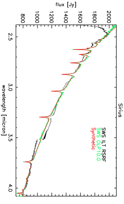
Figure 4: Comparison between the band-1 AOT01 speed-4 observation of Sirius reduced by using the old ILT RSRF’s (black) or the new OLP10 (green) and the synthetic spectrum with stellar parameters T_eff = 10150 K, $\log$ g = 4.30, M = 2.0 M_⊙, z = 0.50, $\xi_{t}$ = 2.0 $\rm{km\,s^{-1}}$, $\mathrm{{}^{12}C/^{13}C}$ = 89, $\varepsilon$(C) = 7.97, $\varepsilon$(N) = 8.15, $\varepsilon$(O) = 8.55 and $\theta_{d}$ = 6.17 mas.

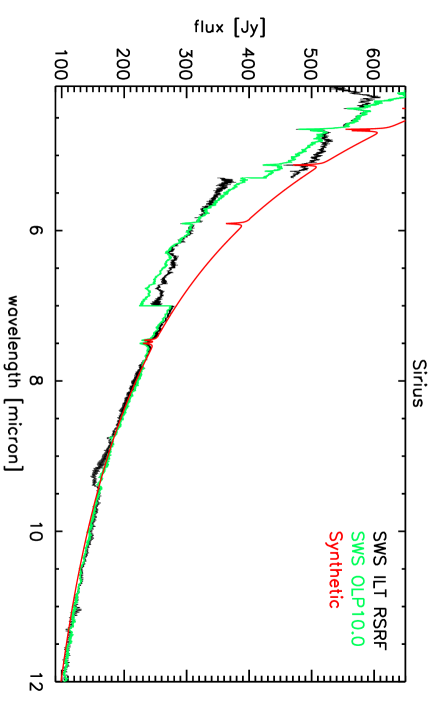
Figure 5: Comparison between the band-2 AOT01 speed-4 observation of Sirius reduced by using the old ILT RSRF’s (black) or the new OLP10 (green) and the synthetic spectrum with stellar parameters T_eff = 10150 K, $\log$ g = 4.30, M = 2.0 M_⊙, z = 0.50, $\xi_{t}$ = 2.0 $\rm{km\,s^{-1}}$, $\mathrm{{}^{12}C/^{13}C}$ = 89, $\varepsilon$(C) = 7.97, $\varepsilon$(N) = 8.15, $\varepsilon$(O) = 8.55 and $\theta_{d}$ = 6.17 mas.

In band 1, the situation is quite clear: Fig. 4 proves that the reduction of ISO-SWS (high-flux) sources has improved seriously during (and after) the ISO-mission. A relative accuracy of better than 2 % is reached in band 1. The discrepancies ($>2\,\%$) still left, e.g. between 3.28 and 3.52 $\mu$m, can be explained by shortcomings of the theoretical predictions.

In band 2, we can see that the calibration has improved w. r. t. previous calibrations, but that still some problems do exist. Due to the new model for memory-effect correction — based on the models of Fouks-Schubert ([Schubert2001]) and developed by Kester ([Kester2001]) — the problems with the memory-effects are now more or less under control, at least when the flux-jump is not too high. Consequently, the RSRFs have changed and improved a lot. The absolute-flux calibration do, however, still predict from time to time a wrong absolute-flux level, especially in bands 2A and 2B, the latter one giving almost consistently across our sample too low a flux level. When concentrating on the relative flux accuracy, one needs to inspect the kind of plots as given for band 2A in Fig. 6 and Fig. 7. The difference between the two figures is situated in the fact that stars are ordered by spectral type in Fig. 6 and by absolute-flux value in Fig. 7. This is necessary to be able to distinguish between problems which are spectral type related — i. e. problems with the theoretical predictions — and problems which are flux, and so memory-effect, related. From an inspection of these figures we can learn that:

• One can clearly see a bump of $\sim 2.5$ % in the wavelength-range from 4.08 – 4.30 $\mu$m. The presence of this bump in hot as well as in cool stars, in low-flux as well as in high-flux sources, is indicative of problems with the RSRF.

• From 4.75 $\mu$m till 4.85 $\mu$m, a slight increase ($\sim 1$ %) is noticeable in both plots. Once more, an indication for a small problem with the RSRFs.

• At the end of band 2A, a quite different behaviour for all the stars emerges. Further inspection indicates that we see a combination of problems with the memory-effect correction, synthetic predictions and, consequently, maybe also with the RSRFs. When we look at Fig. 6, we can recognize a same — increasing — trend for $\beta$ Peg, $\alpha$ Cet, $\beta$ And and $\alpha$ Tau, the coolest stars in our sample and so indicating a problem with the synthetic predictions. This behaviour is however not visible for HD 149447, whose spectral type is in between $\beta$ And and $\alpha$ Tau. An analogous discrepancy is visible for $\delta$ Dra with respect to the stars with almost the same effective temperature. Looking now at Fig. 7, we see that HD 149447 and $\delta$ Dra (together with Vega and $\alpha$ Tuc) have almost the same absolute flux-level in band 2A and show the same trend (decreasing slope) in this plot, indicating a problem with the correction for memory-effects, a statement which is confirmed when we compare the upscan and downscan data.

The majority of discrepancies encountered in bands 2B and 2C are due to still existing problems with the memory-effect correction and smaller problems with the RSRFs. This kind of exercise gives us, however, also an idea on the relative accuracy in band 2: an accuracy of better than 6 % is reached in band 2, which is — taking into account the problematic behaviour of the detectors in band 2 — a very good result! The new extended model for memory-effect correction which is now under development by Kester, in conjunction with a last iteration in the determination of the RSRFs may even improve this number.

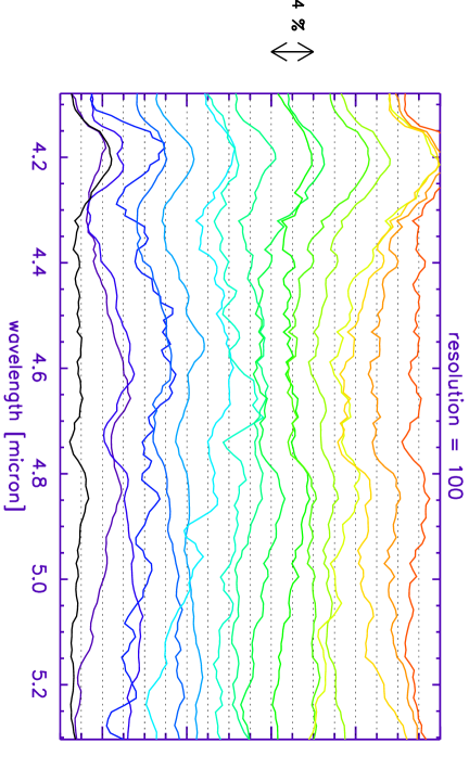
Figure 6: Division between SWS AOT01 data and their theoretical predictions at a resolving power of 100. The synthetic spectra are calculated using as stellar parameters the values determined from the band-1 data. In this figure, the stars are ordered by spectral type. The mean of the different, coloured, divided spectra is given in black at the bottom of the figure.

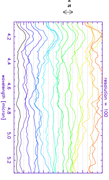
Figure 7: Division between SWS AOT01 data and their theoretical predictions at a resolving power of 100. The synthetic spectra are calculated using as stellar parameters the values determined from the band-1 data. In this figure, the stars are ordered by absolute-flux value. The mean of the different, coloured, divided spectra is given in black at the bottom of the figure.

5 CONFRONTATION WITH THE SEDs OF COHEN

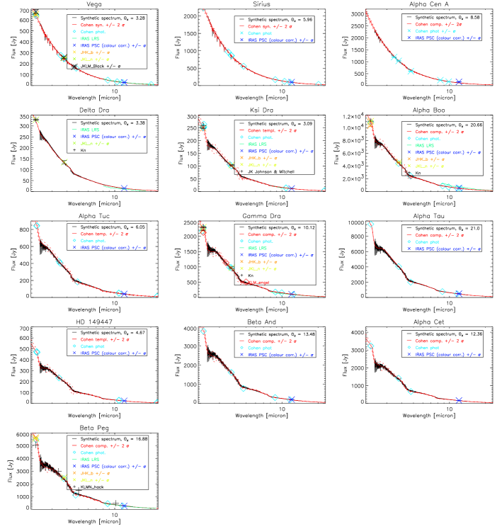
Figure 8: Comparison between the synthetic spectra of the standard stellar sources, their SED of Cohen and various photometric datapoints.

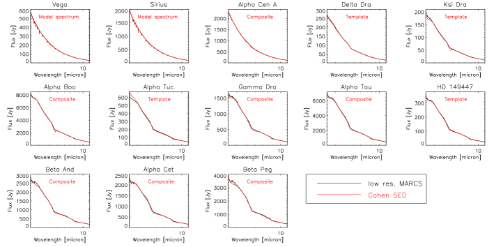
Figure 9: Comparison between the SEDs of Cohen (red) for the standard stellar sources and the synthetic spectra (black) rebinned to the same resolution as the SEDs of Cohen.

Since the SEDs by Cohen ([Cohen et al.1992], [Cohen et al.1995], [Cohen et al.1996], [Witteborn et al.1999]) are used for the calibration of the SWS spectrometers and the synthetic spectra resulting from this project were used to improve the calibration in OLP10, a confrontation between the two sets of data may be instructive. Several stars are in common between the two samples: 1. Vega and Sirius for which Cohen has constructed a calibrated model spectrum; 2. a composite spectrum (i. e. various observed spectra have been spliced to each other using photometric data) is available for $\alpha$ Cen A, $\alpha$ Boo, $\gamma$ Dra, $\alpha$ Tau, $\beta$ And, $\alpha$ Cet and $\beta$ Peg; 3. a template spectrum (i. e. a spectrum made by using photometric data of the star itself and the shape of a ‘template’ star) is built for $\delta$ Dra (template: $\beta$ Gem: K0 III), $\xi$ Dra (template: $\alpha$ Boo: K2 IIIp), $\alpha$ Tuc (template: $\alpha$ Hya: K3 II-III) and HD 149447 (template: $\alpha$ Tau: K5 III). One should notice that for the composite spectrum of $\gamma$ Dra, Cohen didn’t have any spectroscopic data available in the wavelength range from 1.2 $\mu$m till 5.5 $\mu$m. The spectrum of $\alpha$ Tau has therefore been used to construct the composite spectrum of $\gamma$ Dra in this wavelength range. In order to ensure independency of the absolute-flux level of the ISO-SWS data, the angular diameters of the synthetic spectra were determined by using the photometric data of Cohen, JKLM data from Hammersley’s GBPP broad band photometry ([Hammersley2001]), IRAS data and some other published photometric data cited in the IA_SED data-base. A comparison between the (high-resolution) synthetic spectra, SEDs of Cohen and used photometric data is given in Fig. 8. The obtained angular diameters $\theta_{d}$ (in mas) for the stellar sources are mentioned in the legend. To better judge upon the relative agreement of these two data-sets, the synthetic spectra were rebinned to the same resolution as the SEDs of Cohen (see Fig. 9). The most remarkable discrepancies between the two spectra arise in the CO and SiO molecular bands, where the molecular bands are consistently across our sample stronger in the composites of Cohen. Cohen has used low-resolution NIR and KAO data to construct this part of the spectrum. Comparing our synthetic spectra with OLP8.4 ISO-SWS data (whose calibration is not based on our results) and the high-resolution Fourier Transform Spectrometer (FTS) spectrum of $\alpha$ Boo published by [*]LD_hinkle1995 (see Fig. 4.5 in [Decin2000]), we did however see that the strongest, low-excitation, CO lines were always predicted as being somewhat too strong (a few percent at a resolution of 50000 for the FTS spectrum), probably caused by a problem with the temperature distribution in the outermost layers of the theoretical model ([Decin et al.2001c]). Moreover, a comparison between our high-resolution synthetic spectrum of $\alpha$ Boo with its FTS spectrum shows also a good agreement for the high-excitation CO $\Delta v=1$ lines, the low-excitation lines being predicted as too weak. The few percent disagreement between FTS and synthetic spectrum will however never yield the kind of disagreement one sees between the low-resolution synthetic spectra and the SED data. The CO $\Delta v=2$ discrepancy visible in $\gamma$ Dra results from using the $\alpha$ Tau observational KAO data. Since $\alpha$ Tau and $\gamma$ Dra have a different set of stellar parameters, with $\alpha$ Tau having a significant larger amount of carbon, the SED of Cohen for $\gamma$ Dra displays too strong a CO feature. One should also be heedful of this remark when judging upon the quality of the template spectra for $\delta$ Dra, $\xi$ Dra, $\alpha$ Tuc and HD 149447.

As conclusion, we may say that the SED spectra of Cohen are excellent (and consistent) for the absolute calibration of an instrument, but that attention should be paid when using them for relative flux calibration.

6 CONCLUSIONS: LESSONS LEARNED

The purpose of this study was to investigate standard stellar sources observed with ISO-SWS in order to improve the calibration of the SWS spectrometers and to elaborate on new theoretical developments for the modelling of these stars. In spite of the moderate resolution of ISO-SWS, the stellar parameters for the cool giants could be pinned down very accurately from their SWS data. This set of consistent IR synthetic spectra could then be used as input for the OLP10 calibration tools. We could demonstrate that the relative accuracy has by now reached the 2 % level in band 1 and the 6 % level in band 2 for (high-flux) sources observed with ISO-SWS. A comparison with the SEDs of Cohen shows us that this set of 16 synthetic spectra are a necessary completion for an instrumental calibration refined at the highest possible level. This kind of analysis, which has been proven to be very adequate, will be applied to bands 3 and 4 and has opened also new channels of research, not only for other instruments on board ISO, like ISO-CAM, but also for the determination of the sensitivity of future telescopes and satellites, like MIDI and Herschel.

$\alpha$ Lyr,$\alpha$ CMa,$\beta$ Leo,$\alpha$ Car,$\alpha$ Cen A,$\delta$ Dra,$\alpha$ Boo,$\alpha$ Tuc,$\beta$ UMi,$\gamma$ Dra,$\alpha$ Tau,HD 149447, $\beta$ And,$\alpha$ Cet,$\beta$ Peg