Serendipitously Detected Galaxies in the Hubble Deep Field

Abstract

We present a catalog of 74 galaxies detected serendipitously during a campaign of spectroscopic observations of the Hubble Deep Field North (HDF) and its environs. Among the identified objects are five candidate Ly$\alpha$–emitters at $z\raisebox{-0.86108pt}{$\stackrel{{\scriptstyle>}}{{\mbox{\tiny$\sim$}}}$}5$, a galaxy cluster at $z=0.85$, and a Chandra source with a heretofore undetermined redshift of $z=2.011$. We report redshifts for 25 galaxies in the central HDF, 13 of which had no prior published spectroscopic redshift. Of the remaining 49 galaxies, 30 are located in the single–orbit HDF Flanking Fields. We discuss the redshift distribution of the serendipitous sample, which contains galaxies in the range $0.10<z<5.77$ with a median redshift of $z=0.85$, and we present strong evidence for redshift clustering. By comparing our spectroscopic redshifts to optical/IR photometric studies of the HDF, we find that photometric redshifts are in most cases capable of producing reasonable predictions of galaxy redshifts. Finally, we estimate the line–of–sight velocity dispersion and the corresponding mass and expected X–ray luminosity of the galaxy cluster, we present strong arguments for interpreting the Chandra source as an obscured AGN, and we discuss in detail the spectrum of one of the candidate $z\raisebox{-0.86108pt}{$\stackrel{{\scriptstyle>}}{{\mbox{\tiny$\sim$}}}$}5$ Ly$\alpha$–emitters.

1 Introduction

The Hubble Deep Field North (Williams et al., 1996, hereafter W96) ranks among the most thoroughly studied portions of the extragalactic universe. The extremely deep multi–color images obtained with the WFPC2 camera on the Hubble Space Telescope, reaching AB mag $B_{450}\sim 29$ with 0$\stackrel{{\scriptstyle\prime\prime}}{{\mbox{.}}}$1 resolution, have revolutionized our understanding of the faint galaxy population and have yielded diverse new results in observational cosmology. Follow–up observations to the original survey span the electromagnetic spectrum, from the radio (Fomalont et al., 1997; Richards et al., 1998, 2000) to the sub–millimeter (Hughes et al., 1998; Barger, Cowie, & Richards, 2000), to both ground and space–based near infrared (Hogg et al., 1997; Dickinson, 1999, 2000; Thompson, Weymann, & Storrie–Lombardi, 1999) and far infrared (Aussel et al., 1999). Recently, X–ray data have become available (Hornschemeier et al., 2000, 2001), and UV observations with the Space Telescope Imaging Spectrograph are in progress (Gardner, Brown, & Ferguson, 2001). In addition to imaging, numerous groups are pursuing spectroscopic observations of galaxies in the HDF. Cohen et al. (2000) report on a magnitude–limited sample more than 92% complete to Vega mag $R=24$; Steidel et al. (1996a) and Lowenthal et al. (1997) report on color–selected samples of Lyman–break galaxies at $z\sim 3$; while Zepf, Moustakas, & Davis (1997) report on a morphologically selected sample of probable gravitational lenses. See Ferguson, Dickinson, & Williams (2000) for a review of measurements and phenomenology of sources in the HDF across the electromagnetic spectrum.

Consequently, the HDF and the eight adjacent, single–orbit $I_{814}$ Flanking Fields (see W96, Table 2) now constitute a very rich database for the study of galaxy formation and evolution. Early results included the confirmation of a flattening in the slope of the faint elliptical/S0 galaxy number count–magnitude relation (Abraham et al., 1996; Zepf, 1997), as well as the revealed inadequacy of the Hubble sequence as a classification scheme for galaxies fainter than $I_{AB}>24$ mag (Abraham et al., 1996). The selection of four very broad bandpass filters for the WFPC2 observations was driven partly by the desire to identify high–redshift galaxies via the Lyman–break technique. Indeed, this strategy facilitated the discovery of distant galaxies whose Lyman–breaks have been redshifted into the $U$–band (Steidel et al., 1996a; Lowenthal et al., 1997), the $B$–band (Steidel et al., 1999), and beyond (Spinrad et al., 1998; Weymann et al., 1998). The exquisite resolution of the WFPC2 images spurred considerable effort toward quantifying galaxy morphology, leading to the disentanglement of morphological $k$–correction from morphological evolution, and revealing an increase in the fraction of true irregulars at faint magnitudes/high redshift (Bunker, 1999). Most recently, mining of this data–rich field has yielded refined techniques in estimating photometric redshifts (e.g. Fernández–Soto, Lanzetta, & Yahil, 1999) and has produced dramatic implications for the history of star–formation (Madau et al., 1996; Steidel et al., 1999) as well as for the role of dust in the distant universe (Hughes et al., 1998; Ouchi et al., 1999).

We are pursuing a variety of programs to study distant galaxies in the HDF. The primary science from these observations, discussed elsewhere, includes extremely deep ($\sim 10^{\rm h}$) moderate and high–resolution Keck/LRIS spectroscopy of Lyman–break galaxies at $z\sim 3$ aimed at understanding their stellar populations and galactic dynamics (e.g. Bunker et al., 1998), and low–resolution spectroscopy of $B$–band and $V$–band dropouts whose colors suggest a population of galaxies with Lyman–breaks and significant Ly$\alpha$–forest absorption at $z>4$ (Spinrad et al., 1998). In the course of these observations, we have targeted more than 65 galaxies in the HDF and its environs for deep spectroscopy, and in so doing we have serendipitously observed some 125 objects which were located propitiously along the slit of a target. Out of the sample of serendipitous detections, we have determined redshifts for 74 sources, with 25 galaxies in the HDF proper, 30 galaxies in the HDF Flanking Fields, and 19 galaxies beyond but in the vicinity of the Flanking Fields. Thirteen of the detections in the central HDF provided the first ever spectroscopic redshift determinations for those sources.

From the first detection of pulsars to the discovery of the cosmic microwave background, serendipity has historically made significant contributions to astronomy. In extra–galactic astronomy in particular, dramatic serendipitous detections include the discovery of a galaxy cluster at $z=2.40$ (Pascarelle et al., 1996), at least three quasars at $z>4$ (McCarthy et al., 1988; Schneider, Schmidt, & Gunn, 1994; Schneider et al., 2000), and the discovery of the first object at $z>5$ (Dey et al., 1998). Serendipity plays a less dramatic but still significant role in large scale redshift surveys: serendipitous detections make up roughly 8% of the measured galaxies in the complete $K_{s}<20$ mag galaxy sample presented by Cohen et al. (1999). Serendipitous surveys in their own right are efficient, as they require no direct initial allocation of telescope time, and they have proven to be both competitive with and complementary to narrow–band imaging surveys. See Thompson & Djorgovski (1995), Manning et al. (2000), and Stern et al. (2000a) for reports on serendipitous searches for high–redshift Ly$\alpha$ emission.

Though none of the serendipitous detections reported herein constitute singularly momentous discoveries, given the status of the HDF as ranking among the most thoroughly mapped pieces of the extragalactic universe, we would be remiss not to report all galaxy redshifts determined in the course of our observations of this well–studied field. In §2 we discuss the spectroscopic observations and the data reduction. In §3 we describe the redshift determination and the process by which the serendipitously detected galaxies were visually identified. We present the catalog of serendipitously detected galaxies in §4, and we discuss their distribution in redshift space, the comparison between spectroscopic and photometric redshifts, the observed properties of the galaxy cluster at $z=0.85$, the observed properties of the Chandra source at $z=2.011$, and the candidate $z\raisebox{-0.86108pt}{$\stackrel{{\scriptstyle>}}{{\mbox{\tiny$\sim$}}}$}5$ Ly$\alpha$–emitters in §5. Throughout this paper, we adopt an Einstein–de Sitter cosmology with $H_{0}=100\,h_{100}$ km s^-1 Mpc^-1, $q_{0}=0.5$, and $\Lambda=0$. All quoted magnitudes are in the AB system unless otherwise specified.

2 Observations and Data Reductions

Between 1997 February and 2001 February, we obtained deep spectra of photometrically selected high–redshift candidates in the HDF and its environs. The data were taken with the Low Resolution Imaging Spectrometer (LRIS; Oke et al. 1995) at the Cassegrain focus on the 10m Keck I and Keck II telescopes. The camera uses a Tek 2048² CCD detector with a pixel scale of 0$\stackrel{{\scriptstyle\prime\prime}}{{\mbox{.}}}$212 pixel^-1. To maximize observing efficiency, we exclusively used the dual amplifier readout mode. Except for three longslit observations in 1997 February, the data were taken with slitmasks designed to obtain spectra for $\sim 15$ targets simultaneously.

For the vast majority of observations, we used a 150 lines mm^-1 grating blazed at 7500 Å, which produces a $4.8$ Å  pix^-1 dispersion. The spectral coverage with this grating is approximately 4000 Å  to 1 micron, allowing us observe the entire optical window irrespective of the grating tilt or the location of the slit on the slitmask. We used a 300 lines mm^-1 grating blazed at 5000 Å (2.55 Å  pix^-1 dispersion) on one set of observations, a 400 lines mm^-1 grating blazed at 8500 Å (1.86 Å  pix^-1 dispersion) on two sets of observations, and a 600 lines mm^-1 grating blazed at 5000 Å (1.28 Å  pix^-1 dispersion) on one set of observations. For targets within the central HDF (where the astrometric solutions are well–determined), we employed 1$\stackrel{{\scriptstyle\prime\prime}}{{\mbox{.}}}$0 slits, yielding a spectral resolution of $\lambda/\Delta\lambda_{\mbox{\tiny FWHM}}=375$ with the 150 lines mm^-1 grating. For targets outside of the HDF (where the astrometric solutions are less well–determined), we employed 1$\stackrel{{\scriptstyle\prime\prime}}{{\mbox{.}}}$5 slits, yielding a spectral resolution of $\lambda/\Delta\lambda_{\mbox{\tiny FWHM}}=250$ with the 150 lines mm^-1 grating. The minimum set of exposures for any given target was 3 $\times$ 1800s. As the position angle of the slit for a particular target normally changed from observation to observation, only a small number ($\sim 5$) of the serendipitous detections benefited from re–observation.

The most recent set of observations (2001 February) were made with the advent of the LRIS–B spectrograph channel (McCarthy et al., 1998). For these observations, we used the 400 lines mm^-1 grating blazed at 8500 Å in red channel, and a 300 lines mm^-1 grism blazed at 5000 Å (2.64 Å  pix^-1 dispersion) in the blue channel. To split the red and blue channels, we used a dichroic with a cutoff at 6800 Å. Together, the two channels in this set–up afforded a spectral coverage of roughly 3200 Å to 1 micron. Again, we observed the entire optical window, but at almost twice the dispersion of our typical spectrograph configuration.

We used the IRAF package (Tody, 1993) to process both the longslit and the slitmask data, following standard slit spectroscopy procedures. Some aspects of treating the slitmask data were facilitated by a home–grown software package, BOGUS, created by D. Stern, A.J. Bunker, and S.A. Stanford. Wavelength calibrations were performed in the standard fashion using Hg, Ne, Ar, and Kr arc lamps; we employed telluric sky lines to adjust the wavelength zero–point. We performed flux calibrations with longslit observations of standard stars from Massey & Gronwall (1990) taken with the instrument in the same configuration as the relevant multislit observation. However, it should be noted that the absolute scale of the fluxed spectra must be regarded with caution. Not all of the nights were photometric; there may be substantial slit losses in the case of an extended source; small errors in slitmask alignment cause additional light loss; and since the position angle of an observation was set by the desire to maximize the number of targets on a mask, the observations were in general not made at or near parallactic angle. Moreover, in the case of serendipitous detections, it is unlikely that the object is optimally aligned with the slit even when all other parameters are perfect. Fortunately, it is merely the redshift of a given object — not the absolute flux or continuum shape — which is of interest at present.

3 Visual Identifications and Redshift Determinations

3.1 Visual Identifications

A serendipitous detection in spectroscopic data presents two challenges to the observer: (1) to locate on an image of the field the progenitor of the spectroscopic signature, and (2) to determine the nature of the object and, where possible, its redshift. We now address the former problem; we discuss the latter in the following section.

In some respects, the process of cataloguing serendipitous detections proceeds backwards from the usual steps involved in compiling redshifts. Generally, one begins with photometry for a galaxy whose location is known and subsequently obtains a spectrum. In our case, we began with a spectrum and worked backward to the progenitor’s location and photometry. To accomplish this task, we combined what was known about the observation — the location of the target, the dimensions and orientation of the target slit, and the position of the target within the slit — and we reconstructed the position of the slit on the sky. We then mapped the reconstructed slit image to the target field and thereby identified a posteriori the objects which we in fact observed.

In the most favorable cases, the two–dimensional spectra contained multiple serendipitous detections. By comparing the relative spatial separations between continuum detections in the two–dimensional spectra to the separations between sources on the slit image, we could uniquely identify each of the progenitors. Even under unfavorable circumstance, in which the target was too faint to appear in the spectrum or was mis–aligned with the slit, the progenitor of a lone serendipitous detection could be identified by comparing its position on the two–dimensional spectrum to its position in the image relative to the edges of the slit.

To this end, the galaxies in the sample divide into two categories: those within the central HDF, and those without. For galaxies inside of the central HDF, we made the visual identification by mapping the slit image to the remarkably deep, well–resolved central $I_{814}$ images presented in W96. We label the galaxies in Table 2 by their IDs, isophotal magnitudes, and positions as given in that paper. If, on the other hand, the target slit extended outside of the central HDF, we relied on supporting photometry provided by the single–orbit $I_{814}$ Flanking Field images of W96, the deep Hawaii 2.2m $V$, $I$, $H+K$ images of Barger et al. (1999, hereafter B99), or the deep $U_{n}$, $G$, $\cal{R}$ images of Steidel et al. (1996b). Since there is no existing nomenclature for sources beyond the central HDF, we adopted a labeling scheme in Table 3 based on the galaxy positions.

To facilitate this position–based nomenclature for serendipitous observations of galaxies in the Flanking Fields and beyond, we computed an astrometric solution to the Hawaii 2.2m $I$–band image of B99. From a fit to 72 objects in a 10^′  $\times$ 10^′  portion of the digitized POSS–II plates (obtained via the Digitized Sky Survey), we found a platescale of 0$\stackrel{{\scriptstyle\prime\prime}}{{\mbox{.}}}$189 pixel^-1 and an orientation angle of 0.630^∘, both of which are consistent with the values reported by B99. The dispersion in the fit was 0$\stackrel{{\scriptstyle\prime\prime}}{{\mbox{.}}}$22 in the right ascension (RA) direction and 0$\stackrel{{\scriptstyle\prime\prime}}{{\mbox{.}}}$26 in the declination (Dec) direction, giving a total error of 0$\stackrel{{\scriptstyle\prime\prime}}{{\mbox{.}}}$37. This error is comparable to the error reported by B99. As a check to the fit, we compared the RA and Dec positions of 10 objects in the central HDF as given by W96 against our newly computed Hawaii 2.2m $I$–band positions and found a mean absolute offset of 0$\stackrel{{\scriptstyle\prime\prime}}{{\mbox{.}}}$11 in RA and 0$\stackrel{{\scriptstyle\prime\prime}}{{\mbox{.}}}$16 in Dec, for a total mean offset of 0$\stackrel{{\scriptstyle\prime\prime}}{{\mbox{.}}}$20. This error is smaller than the sum in quadrature of the total dispersion in our fit and the accuracy of the W96 absolute astrometry (reported as good to approximately 0$\stackrel{{\scriptstyle\prime\prime}}{{\mbox{.}}}$4), suggesting that our reported RA and Dec positions themselves are good to roughly 0$\stackrel{{\scriptstyle\prime\prime}}{{\mbox{.}}}$4.

In three cases, the serendipitous detection fell outside of the Hawaii 2.2m fields. To visually identify these objects, we utilized our own 70 minute $R$–band image taken with the Echelle Spectrograph and Imager (ESI, Sheinis et al., 2000) on UT 2000 May 05. See Stern et al. (2000b) for a detailed account of the observation and data reduction. The astrometric solution for the position–based nomenclature was determined exactly as described for the Hawaii 2.2m image; $I_{\mbox{\tiny AB}}$ magnitudes are not available for these detections. In five cases, the progenitor of a serendipitous spectroscopic detection was too faint to be detected in any of the supporting imaging. Nonetheless, we were able to estimate a position for the source by extrapolating from the known position of the target and the dimensions and orientation of the target slit. We have indicated such cases on Table 3.

3.2 Redshifts

For each member of the serendipitous catalog, we measured the redshift by visually inspecting the spectrum and noting the wavelengths of spectral features. For objects with multiple strong emission lines, the proper interpretation of the spectral features was unambiguous and the assignment of their rest wavelengths was straightforward. The situation was more difficult for faint objects showing only absorption lines. If such a spectrum did not conform to the standard pattern of Balmer lines and the H$+$K Ca II doublet seen in the vicinity of the 4000 Å–break (D4000), then it was generally impossible to determine a redshift.

The most common type of serendipitous detection involved the presence of a single emission line, the interpretation of which can problematic. In general, a single, isolated line could be any one of Ly$\alpha$, [O II] $\lambda$3727, H$\beta$, [O III] $\lambda$5007, or H$\alpha$, though given sufficient spectral coverage, most erroneous interpretations can be ruled out. For instance, the absence of H$\beta$ or [O III] $\lambda$4959 serves to discount the interpretation of a solo line as [O III] $\lambda$5007. Similarly, lines that are bluer than rest H$\alpha$ cannot be H$\alpha$ themselves, and the presence of H$\beta$ or [O III] $\lambda$5007 would be expected for a solo line redder than rest H$\alpha$ (but see Stockton & Ridgway 1998). Hence, the primary threat to determining one–line redshifts is the potential for mis–identifying Ly$\alpha$ as [O II] $\lambda$3727 or vice versa. Unfortunately, with low dispersion spectra it is often impossible to distinguish between the high equivalent width forms of these emission lines without a pronounced continuum depression or a line asymmetry, both characteristic of Ly$\alpha$. For two accounts of the potential pitfalls associated with one–line spectroscopic redshift identifications, see Stern et al. (2000a) and Manning et al. (2000).

In part to reflect the uncertainty in interpreting solo lines, we divide the serendipitous detections into five spectral categories (SC) based on their general morphology. Table 1 lists the spectral categories with a brief description of each. The spectra of category 1 sources show multiple features which can be uniquely identified, yielding secure redshift determinations. The spectra of category 2 sources show a solo emission line in the presence of strong continuum both redward and blueward of the line. Such lines were identified as [O II] $\lambda$3727, and the redshift determination is considered secure. The spectra of category 3 sources show a solo emission line redward of a strong continuum break. Such lines were identified as Ly$\alpha$ and the continuum breaks were interpreted as the onset of absorption by the Ly$\alpha$–forest (which causes significantly diminished flux shortward of 1216 Å). Of course, especially in star–forming systems, the continuum in the vicinity [O II] $\lambda$3727 can also show a break — the Balmer break at 4000 Å — and in cases of low signal–to–noise, the morphology of the Balmer break alone is not sufficient to distinguish it from the break at Ly$\alpha$. Fortunately, for galaxies at $z\raisebox{-0.86108pt}{$\stackrel{{\scriptstyle>}}{{\mbox{\tiny$\sim$}}}$}4$, the break at Ly$\alpha$ is expected to be of greater amplitude than the largest observed D4000 amplitudes (see Stern & Spinrad, 1999, Fig. 12), so the two features can be easily discerned. At lower redshifts, however, the amplitude of the two breaks may be comparable, and without corroborating spectral features the redshift identification is largely subjective. Of five category 3 sources in this catalog, two are at $z\raisebox{-0.86108pt}{$\stackrel{{\scriptstyle>}}{{\mbox{\tiny$\sim$}}}$}4$, one has a redshift which is confirmed by other authors, and one has supporting photometric redshifts from two other authors; their redshift determinations are considered secure. The redshift of the remaining category 3 source should be considered tentative, as indicated on Table 3. Example spectra for categories 1, 2, and 3 are shown in Figure 1.

The spectra of category 4 objects show an isolated emission in the absence of any continuum, which generally suggests a weak detection of either [O II] $\lambda$3727 or Ly$\alpha$. Clearly, the confidence one can exercise in discriminating between these two cases is a strong function of the robustness of the detection, the resolution of the spectrum, and the availability of supporting imaging. See §5.5 for a detailed discussion of the redshift determination of a typical category 4 source. Example spectra for both interpretations of category 4 sources are shown in Figure 2. The spectra of category 5 sources show a continuum break. Such breaks were classified as either the Balmer break or as Ly$\alpha$–forest absorption according to the strength of the continuum blueward of the break. Example spectra for both interpretations of category 5 are shown in Figure 3. The redshift determinations of both category 4 and category 5 sources are considered secure unless otherwise indicated. Serendipitous detections about which we were unable to attain a reasonable degree of confidence were omitted from the catalog; nearly half of the initial sample of 121 serendipitous detections were rejected for this reason.

To minimize the possibility that we mis–classified the solo emission line of a low–redshift category 4 source as high–redshift Ly$\alpha$, we checked that the source as visually identified in the Hawaii 2.2m $I$–band image of B99 did not also appear in the $\cal{R}$–band image of Steidel et al. (1996b). In this fashion, we ensured that the $\cal{R}$–band flux of the source in question was severely attenuated by the hydrogen forest, consistent with $z\raisebox{-0.86108pt}{$\stackrel{{\scriptstyle>}}{{\mbox{\tiny$\sim$}}}$}4$. We discovered one erroneous redshift determination with this technique: F 36265–1443 was marginally detected in 1999 June such that [O III] $\lambda$5007 appeared in the two–dimensional spectrum as a solo emission line at $\lambda=8136$ Å, and the line was initially mis–classified as high–redshift Ly$\alpha$ at $z=5.691$. However, the presence of the progenitor in the $R$–band image of Steidel et al. (1996b) ruled out the tantalizing high–redshift interpretation, and subsequent targeted spectroscopy revealed a spectrum with [O II] $\lambda$3727, [O III] $\lambda$4959, [O III] $\lambda$5007, H$\beta$, and H$\gamma$ in emission at $z=0.625$.

In the event that a redshift for a serendipitous detection remained undetermined, one possibility is that the object lies in the so–called “redshift desert,” the interval spanning roughly $1.7<z<2.3$. The limits of this interval are set by the fact that at higher redshifts Ly$\alpha$ would fall on the detector, and at lower redshifts the oxygen lines and/or the Balmer lines would fall on on the detector. At intermediate redshifts, however, there is a dearth of prominent spectral features, rendering redshift determination difficult. A second possibility is that the object does have spectral features which are in principle observable, except that the features fall in a region heavily contaminated by night sky emission. As sky subtraction is particularly problematic at $\lambda>7200$ Å for low signal–to–noise, low dispersion spectra, it is reasonable to conclude that at least a few redshifts were lost to this effect.

It should be noted that for the $\sim 5$ cases in which a single galaxy was multiply observed, the agreement in the individual redshifts was excellent. Discrepancies never exceeded $\Delta z=0.004$.

4 The Catalogs

We present the catalog of serendipitously detected galaxies in Table 2 and Table 3. Table 2 contains 25 galaxies located in the HDF proper, identified by their W96 number as described in the preceding section. The $I_{814}$ magnitude is the isophotal magnitude given by W96, and the RA and Dec are J2000 coordinates, also given therein. The spectral category was assigned as described in §3.1; also see Table 1. Table 3 contains 49 galaxies located outside the central HDF, identified by their positions as described in the preceding section. The 30 galaxies located in the HDF Flanking Fields are indicated. The isophotal $I_{\mbox{\tiny AB}}$ magnitudes were determined by running the source extraction algorithm SExtractor (Bertin & Arnouts, 1996) on the Hawaii 2.2m $I$–band image of B99. We estimated the $I_{\mbox{\tiny AB}}$ zero–point by using stars in the central HDF; as such, the uncertainty in the $I_{\mbox{\tiny AB}}$ is $\sim 0.3$ mag. All spectral lines in both tables are emission lines unless otherwise noted.

5 Discussion

The 74 galaxies in the serendipitous catalog span the redshift range $0.10<z<5.77$, with a median redshift of $z=0.85$. The vast majority of the galaxies are emission-line systems; 5% of the sample show only absorption lines. This bias stems from the diminished likelihood of serendipitously detecting an absorption–line system with sufficient signal–to–noise to allow the redshift to be determined.

We estimate that the uncertainty in the most secure redshifts (SC 1) is $|\Delta z|\approx 0.003$. The uncertainty in redshifts based on solo emission lines or continuum breaks (SC 2 to 5) — assuming the identification of the spectral feature is sound — is $|\Delta z|\approx 0.004$. For the 12 galaxies in the central HDF also observed spectroscopically by Cohen et al. (1996), Cohen et al. (2000), Phillips et al. (1997), or Steidel et al. (1996a), we compared our spectroscopic redshift to the published value and found that the agreement was excellent, with a mean deviation of $|\Delta z|=0.001$ and a dispersion of $\sigma_{\Delta z}=0.001$. In all cases, the discrepancy is comparable to our estimated measurement error.

5.1 The Redshift Distribution

The redshift distribution of the serendipitous catalog, compared with a “total sample” consisting of this sample, all published redshifts for galaxies in the central HDF, and 26 published redshifts for galaxies flanking the central HDF, is shown in Figures 4 and 5. Sources for the total sample are Bunker et al. (1998); Cohen et al. (1996); Cohen et al. (2000); Lowenthal et al. (1997); Phillips et al. (1997); Spinrad et al. (1998); Stern & Spinrad (1999); Waddington et al. (1999); and Weymann et al. (1998). The histogram displayed in Figure 4 displays the total range of redshifts of the combined catalogs, $0.089<z<5.77$, with a comparatively coarse resolution of $\Delta z=0.1$. Given the caveat that we are insensitive to galaxies in the redshift range $1.7<z<2.3$ (cf. §3.1), we find that the redshift distribution of the serendipitous sample closely follows that of the total sample.

To investigate the redshift clustering properties of the serendipitous sample, we display the redshift distribution for the galaxies in the range $0<z<1$ with a resolution of $\Delta z=0.01$ in Figure 5. The figure shows clear evidence of clustering in both the serendipitous sample and the total sample. Moreover, the clustering present in the total sample is mirrored almost perfectly by that present in the serendipitous sample. Assuming a fixed number of galaxies per redshift bin (i.e. no evolution in bin membership with redshift), we find a $2.3\sigma$ peak in the serendipitous sample at $z=0.79$, a $3.2\sigma$ peak at $z=0.56$ and $z=0.68$, and a $6.9\sigma$ peak at $z=0.85$. In total, we find that 17 out of the 51 serendipitous galaxies (33%) fall into peaks significant at greater than 97.5% confidence. This figure compares favorably with that of Cohen et al. (1996, hereafter C96), who find that 57 out of 140 (41%) of their sample of spectroscopically observed HDF galaxies fall into redshift peaks. That the locations of our peaks vary somewhat from those in C96 is not surprising. Whereas C96 chose redshift bins of variable centers and widths so as to maximize their significance relative to occurring by chance in a smoothed velocity distribution, we chose fixed bin centers and widths, cf. Phillips et al. (1997). Even so, our peaks centered on $z=0.56$ and $z=0.68$ no doubt reflect the same structures revealed by the peaks in C96 at $z_{p}=0.559$ and $z_{p}=0.680$, respectively. We find no evidence of periodicity in the peak redshifts, as described by Broadhurst et al. (1990).

Beyond the strong evidence of redshift clustering, there are two outstanding features of the redshift distribution of the serendipitous sample. First, there is a relative deficiency of serendipitous detections at $z<0.4$. Second, the redshift peak centered on $z=0.32$ evident in the total sample is not represented in the serendipitous sample. Taken together, these features appear to suggest a selection effect which excludes galaxies at $z<0.4$ from serendipitous detection. However, since this redshift range is perfectly accessible to LRIS via the Balmer lines and by [O II] and [O III] emission, it is likely that the scarcity of low–redshift galaxies in the serendipitous catalog is merely the combined effect of: (1) the increasingly small cosmological volume surveyed at low–redshift, (2) the comparatively small size of the serendipitous catalog, and (3) the fact that the HDF was selected to be devoid of bright galaxies in the first place. At a minimum, these facts make it impossible to comment on the significance of the apparent $z<0.4$ deficiency.

5.2 A Check of Photometric Redshifts

Photometric redshift techniques have become an essential tool of observational cosmology, with applications ranging from determining luminosity functions to selecting high–redshift candidates for spectroscopy. We have utilized our set of spectroscopic redshifts for 23 of the 25 serendipitously detected galaxies in the central HDF to carry out a test of the photometric redshifts presented by Fernández–Soto, Lanzetta, & Yahil (1999), who employ a maximum–likelihood analysis applied to spectral energy distribution–fitting of precise $U_{300}$, $B_{450}$, $V_{606}$, $I_{814}$, $J$ (1.2 $\mu$m), $H$ (1.65 $\mu$m), and $K$ (2.2 $\mu$m) photometry. For two galaxies, HDF 4–402.1 and HDF 4–236.0, no photometric redshift was available, no doubt owing to their faintness: $I_{\mbox{\tiny AB}}=24.96$ and 28.26, respectively. The sample of predicted redshifts was taken from the group’s world wide web site — the University of New South Wales/State University of New York at Stony Brook HDF Clickable Map — which is an interactive version of the catalog presented in the associated paper.

We compare the spectroscopic redshift ($z_{\mbox{\tiny spec}}$) and the photometric redshift ($z_{\mbox{\tiny phot}}$) in a scatter plot of $z_{\mbox{\tiny spec}}$ versus $z_{\mbox{\tiny phot}}$ for redshifts less than 1.5 in Figure 6. There are three obvious errors in the photometric redshifts: (1) HDF 4–639.1, listed with $\mbox{$z_{\mbox{\tiny spec}}$}=2.592$ and $\mbox{$z_{\mbox{\tiny phot}}$}=0.000$, whose spectrum shows Ly$\alpha$ in emission with a strong continuum break (SC 3), and whose $z_{\mbox{\tiny spec}}$ is confirmed by both Steidel et al. (1996a) and Cohen et al. (2000); (2) HDF 2–600.0, listed with $\mbox{$z_{\mbox{\tiny spec}}$}=0.425$ and $\mbox{$z_{\mbox{\tiny phot}}$}=1.800$, whose spectrum shows a strong solo emission line interpreted as [O II] $\lambda$3727 (SC 4); and (3) HDF 4–658.0, listed with $\mbox{$z_{\mbox{\tiny spec}}$}=0.558$ and $\mbox{$z_{\mbox{\tiny phot}}$}=4.320$, whose spectrum shows both [O II] and [O III] emission (SC 1). These outliers comprise 13% of the sample, roughly consistent with the finding of Cohen et al. (2000) that outliers at more than 4$\sigma$ in the $z_{\mbox{\tiny spec}}$–$z_{\mbox{\tiny phot}}$ plane comprised $\sim 10$% of the subset of galaxies at $z<1.5$. The outliers are not shown in Figure 6, as they are off the scale.

The mean and the dispersion of the difference between the predicted photometric redshifts and the measured spectroscopic redshifts are $|\Delta z|=0.380$ and $\sigma_{\Delta z}=0.907$, respectively. However, these values are dominated by the three discrepant points described above. When the discrepant points are omitted, we find a mean deviation of $|\Delta z|=0.098$ and a dispersion of $\sigma_{\Delta z}=0.010$. These errors are consistent with the assessment that cosmic variance (the fact that the model spectra used in determining photometric redshifts represent a finite sample of all possible galaxy spectra) rather than photometric errors is the dominant source of error at small redshift (Fernández–Soto, Lanzetta, & Yahil, 1999). Moreover, these results confirm that — barring catastrophic errors — photometric redshifts are capable of producing reasonable predictions of galaxy redshifts where suitably precise multicolor photometry is available.

5.3 A Galaxy Cluster at $z=0.85$

We report the serendipitous discovery of ClG 1236+6215, a galaxy cluster with redshift $z=0.85$ nominally centered at $\alpha=$12^h36^m39$\stackrel{{\scriptstyle\prime\prime}}{{\mbox{.}}}$6, $\delta=+$62^∘15^′54^′′ (J2000). The cluster was initially identified as an over–density of centrally concentrated red objects in a small region to the northwest of the HDF in the deep Hawaii 2.2m $V$ and $I$ images of Barger et al. (1999). In a circle of radius 45 arcsec centered on the cluster position, the density of objects with $(V-I)_{\mbox{\tiny AB}}>1.5$ is 18 arcmin^-2, versus a density of only 6.5 arcmin^-2 over the rest of the 90 arcmin² Hawaii 2.2m field. We interpreted the $(V-I)_{\mbox{\tiny AB}}$ color of the concentration to be the result of the 4000 Å break redshifted into the $I$–band, and we targeted five of the reddest members for spectroscopy. All five of the targets proved to have redshifts very near to $z=0.85$. We added three more redshifts by selecting objects from the redshift catalog of Cohen et al. (2000) which had $(V-I)_{\mbox{\tiny AB}}>1.5$ and $0.84<z<0.86$, and which were located within 45 arcsec ($0.17\,h_{100}^{-1}$ Mpc) of the cluster center. Together, the eight spectroscopic members of ClG 1236+6215 yield a mean redshift for the cluster of $z=0.849\pm 0.004$. The properties of the spectroscopic members of ClG 1236+6215 are summarized in Table 4.

Following the prescription of Harrison (1974) for properly considering the contributions to measured redshifts due to the radial component of the motion of our Galaxy with respect to the Local Group, to the cosmological expansion between comoving observers at our Galaxy and at the galaxy cluster, and to the radial component of the peculiar velocity of the galaxy within the cluster, we calculated an estimate of the corrected line–of–sight velocity dispersion $\sigma_{\mbox{\tiny$\parallel$}}$ in ClG 1236+6215. We followed the treatment of Danese, De Zotti, & di Tullio (1980) to account for the spurious systematic contribution to $\sigma_{\mbox{\tiny$\parallel$}}$ from measurement errors in the member redshifts. Assuming an underlying Gaussian distribution for the galaxy velocities, we found $\mbox{$\sigma_{\mbox{\tiny$\parallel$}}$}=610\pm 190$ km s^-1 (68% confidence); this value should be treated with caution due to the small number of spectroscopic members. Beers, Flynn, & Gebhardt (1990) point out that the classical standard deviation estimator for cluster velocity dispersions is neither resistant to the presence of outliers nor robust for non–Gaussian underlying populations. However, employing the “gapper” method as implemented in their ROSTAT package yields a correction which is less than our estimated uncertainty.

In the limiting isothermal model, the calculated velocity dispersion translates to a mean cluster mass within a 45 arcsec ($0.17\,h_{100}^{-1}$ Mpc) radius of the cluster center of $M(r<0.17\,h_{100}^{-1}\mbox{ Mpc})=2.6\times 10^{13}\,h_{100}^{-1}\,M_{\odot}$. For comparison with other authors, the mean mass within the Abell radius is $M(r<1.5\,h_{100}^{-1}\mbox{ Mpc})=2.3\times 10^{14}\,h_{100}^{-1}\,M_{\odot}$. Of perhaps more immediate observational consequence is the X–ray luminosity expected for the given velocity dispersion. Drawing on a sample of 197 galaxy clusters — which constitutes the largest cluster data set used to date for such a study — Xue & Wu (2000) find $L_{X}/(10^{43}\mbox{ erg s}^{-1})=10^{-13.68\pm 0.61}\mbox{$\sigma_{\mbox{\tiny$\parallel$}}$}^{5.30\pm 0.21}$ for the X–ray bolometric luminosity–velocity dispersion relation. This result yields an expected X–ray bolometric luminosity for ClG 1236+6215 of $L_{X}=1.2\times 10^{44}$ erg s^-1, a value which exceeds the expected detection threshold of the upcoming $\approx 1$ Ms Chandra X–ray Observatory (CXO) exposure of the HDF and its environs (Brandt, 2001).

5.4 Optical Spectroscopy of the X–ray Source CXOHDFN J123635.6$+$621424

Optical spectroscopy of faint X–ray sources is the key to determining the poorly understood physical properties of the population responsible for producing the X–ray background. We present the first published optical spectrum and redshift for CXOHDFN J123635.6$+$621424, a well–observed X–ray source identified with a face–on spiral galaxy at $z=2.011$, fortuitously located in the Inner West HDF Flanking Field.

CXOHDFN J123635.6$+$621424 was first detected as a weak radio source (8.15 $\mu$Jy at 8.5 GHz; 87.8 $\mu$Jy at 1.4 GHz) in the sensitive HDF radio surveys of Richards et al. (1998, 2000). The source has a comparatively steep radio spectral index ($S_{\nu}\propto\nu^{-\alpha}$; $\alpha^{\mbox{\tiny 8.4 GHz}}_{\mbox{\tiny 1.4 GHz}}>0.87$), and the radio emission extends across 2$\stackrel{{\scriptstyle\prime\prime}}{{\mbox{.}}}$8. In general, microjansky radio emission from disk galaxies can result from either star formation (e.g. from free–free emission originating in H II regions) or from AGN activity connected with a central engine. Richards et al. (1998, 2000) argued that (1) in the case of a central AGN powering a weak ($P<10^{25}$ W Hz^-1) radio source, the bulk of the radio emission is confined to the nuclear region and is therefore characterized by sub–arcsecond angular scales, and (2) such small scales result in a high opacity to synchrotron self–absorption, yielding flat or inverted spectral indices typically in the range $-0.5<\alpha<0.5$. Hence, the origin of the radio emission in CXOHDFN J123635.6$+$621424 was taken to be extended star–forming regions. This conclusion was ostensibly borne out by an Infrared Space Observatory Camera (ISOCAM) detection of the source (Aussel et al., 1999). If the source were a moderate–to–low redshift starburst galaxy (as suggested by Hornschemeier 2001, owing to the object’s spatial extent), the ISOCAM 15 $\mu$m filter (LW3) would sample rest wavelengths from roughly 6 $\mu$m to 12 $\mu$m; the mid–infrared emission could therefore be plausibly attributed to the unidentified infrared bands (UIB) and to the hot, 200 K dust which typically dominates the spectral energy distribution of starbursts over those wavelengths (Aussel et al., 1999).

In contradistinction to the foregoing conclusions, both the optical and X–ray properties of CXOHDFN J123635.6$+$621424 indicate the presence of AGN activity. The optical spectrum shows moderate–width ($\sim 1000$ km/s), high–ionization emission lines, similar to those of the recently reported quasar II in the Chandra Deep Field South (Norman et al., 2000) and typical of high–redshift radio galaxies (cf. McCarthy et al., 1993; Stern & Spinrad, 1999). We detect Ly$\alpha$, N V $\lambda$1240, Si IV $\lambda$1397, C IV $\lambda$1549, He II $\lambda$1640, C III] $\lambda$1909, [Ne IV] $\lambda$2424, and Mg II $\lambda$2800 (Figure 7). Moreover, the rest frame equivalent widths of the C III] $\lambda$1908 and C IV $\lambda$1548 emission lines ($\sim 13$ Å and $\sim 100$ Å, respectively) are within the ranges found in multiple AGN emission line surveys and optical/radio quasar surveys (see Lehmann et al., 2000, and references therein). We also note that the C IV $\lambda$1549/He II $\lambda$1640 ratio of $\sim 8$ is more typical of quasars than of radio galaxies. Optical and near–IR photometry of CXOHDFN J123635.6$+$621424 corroborates these findings. Hogg et al. (2000) give $({\cal R}-K_{s})=4.74$ for the source, and Hasinger et al. (1999) report that all X–ray counterparts with $(R-K^{\prime})>4.5$ in their ROSAT Ultra Deep HRI Survey are either members of high redshift clusters or are obscured AGN. Finally, CXO observations of the source indicate a comparatively hard X–ray spectrum — the definitive signature of an AGN. The X–ray band ratio, defined as the ratio of hard–band (2 keV to 8 keV) to soft–band (0.5 keV to 2 keV) number counts, is $0.75^{+0.71}_{-0.43}$, corresponding to a photon index of $\Gamma=0.75$ (Hornschemeier et al., 2001).

When re–interpreted in the light of the spectroscopic redshift, even the mid–IR data for CXOHDFN J123635.6$+$621424 actually indicate the presence of an AGN. For the derived redshift of $z=2.011$, the ISOCAM LW3 filter samples rest wavelengths spanning only 4 $\mu$m to 5 $\mu$m. Here, the contribution to the mid–IR spectral energy distribution made by UIB emission and by dust at 200 K is severely attenuated (see Aussel et al., 1999, Figure 1). Hence, the ISOCAM detection of this source is far more plausibly explained by the hot, $\sim 10^{3}$ K dust found in the central region of an AGN (e.g. see Aussel et al., 1998) rather than by star formation alone. The weakness of Ly$\alpha$ in this galaxy substantiates the presence of dust in this system.

Though the canonical wisdom regarding extended radio sources with spectral indices steeper than $\alpha>0.5$ dictates that such sources are driven by starbursts (Richards et al., 1998, 2000; Hornschemeier et al., 2001), the combined weight of evidence from X–ray, optical, and near– and mid–IR observations of CXOHDFN J123635.6$+$621424 is definitively in favor of an obscured AGN. This conclusion is consistent with the trend reported by Hornschemeier et al. (2001): that the high X–ray luminosities and large band ratios of several CXO–detected radio sources previously reported as starburst–type objects strongly suggests the presence of heretofore unidentified AGNs. We are currently pursuing Keck/NIRSPEC spectroscopy of this interesting source in order to further detail its physical properties.

5.5 Galaxies at $z\stackrel{{\scriptstyle>}}{{\sim}}5$

In the course of deep, targeted spectroscopy of photometric high–redshift galaxy candidates, we have identified several serendipitous high–redshift Ly$\alpha$–emitting candidates, including five sources at $z\raisebox{-0.86108pt}{$\stackrel{{\scriptstyle>}}{{\mbox{\tiny$\sim$}}}$}5$. These high–redshift sources are evident in Figure 4, and they are listed in Table 3. The surface density of such sources is sufficiently high that these discoveries are not unexpected (e.g. Dey et al., 1998; Manning et al., 2000). Indeed, slit spectroscopy surveys for high–redshift Ly$\alpha$ emission are fully complimentary to narrow–band searches (e.g. Hu, Cowie, & McMahon, 1998; Steidel et al., 1999; Rhoads et al., 1999): rather than probing a large area of sky for objects over a limited range of redshift, deep slit spectroscopy surveys a small area of sky for objects over a large range in redshift (Pritchet, 1994; Thompson & Djorgovski, 1995). The total area covered by the spectroscopic slits during the course of our study was $\approx 2.2$ arcmin², implying a surface density of $\approx 2.3$ arcmin^-2 Ly$\alpha$–emitters at redshift $z\sim 5$. This value is roughly consistent with the surface density of high–redshift Ly$\alpha$–emitters reported by Cowie & Hu (1998): $\approx 3$ arcmin^-2 (unit–$z$)^-1 at redshift $z\sim 3.4$, for comparable sensitivity to line flux. Of course, one should exercise caution regarding these values, owing to the small number of detections involved.

Each of the high–redshift sources in this catalog are solo emission line sources (SC 4), and as indicated by a handful of cautionary tales (§3.2 herein; also see Stockton & Ridgway, 1998; Stern et al., 2000a), such redshift identifications should be greeted with a degree of circumspection. A detailed discussion of each individual source is beyond the scope of this paper, and a separate manuscript is planned. For now, we restrict the discussion to one likely high–redshift source, F 36246–1511 at $z=5.631$, as illustrative of the situation.

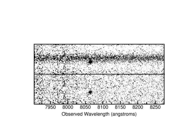
Figure 8: Discovery spectrogram for F 36246–1511, a solo emission line source interpreted as a Ly$\alpha$–emitter at $z=5.631$, lensed by an absorption–line galaxy (F 36247–1510) at $z=0.641$. The top panel shows the raw spectrogram. The bottom panel shows the solo emission line after subtracting a Gaussian fit to the foreground continuum source. The fit was made to the continuum source blueward of the emission line so that after subtraction — assuming a locally flat spectrum for both sources — any remaining flux could be attributed to the solo line–emitter. The total exposure time is 5.4 ks. Each panel is 9$\stackrel{{\scriptstyle\prime\prime}}{{\mbox{.}}}$5 in height. Since the discovery spectrum was obtained, we have targeted F 36246–1511 for an additional $\sim$ 25 ks of spectroscopy. The resulting composite spectrum, which confirms the high–redshift interpretation, will appear in a future work.

F 36246–1511 was discovered in a 5400s exposure obtained on UT 19 February 1998. The source appeared as solo emission line spatially offset by $\sim 2^{\prime\prime}$ from an absorption–line galaxy (F 36247–1510; $z=0.641$). A portion of the two–dimensional spectrogram, centered on the emission line, is shown in Figure 8. The top panel shows the original two–dimensional spectrogram; the continuum of the absorption–line galaxy and the spatially offset emission line can be readily seen. In the bottom panel, we have subtracted a Gaussian fit to the foreground continuum source. The fit was made to the continuum source only blueward of the emission line so that after subtraction — assuming a locally flat spectrum for both sources — any remaining flux could be attributed to the high–redshift candidate. In this fashion we hoped to isolate continuum flux from the high–redshift source and recover a continuum break, which would lend credence to the Ly$\alpha$–interpretation. However, as can be seen in the one–dimensional extracted spectrum (Figure 9), the continuum break is of low significance relative to the noise.

As the emission line itself is not obviously asymmetric, the remaining evidence in favor of the Ly$\alpha$–interpretation is two–fold. To begin, the observed frame equivalent width of the line is $\sim 300$ Å. This value exceeds the largest equivalent widths observed for other likely interpretations: 200 Å for the H$\alpha+$[N II] complex; 100 Å for [O III] $\lambda$5007; and 100 Å for [O II] $\lambda$3727 (Stern & Spinrad, 1999). Additionally, a faint source is visible in the Outer West $I_{814}$ Flanking Field image (W96) located at the correct separation and orientation to be the progenitor of the solo emission line. Unfortunately, as the offset between the foreground continuum source and the high–redshift candidate is only $\sim 2^{\prime\prime}$, ground–based images are insufficient to resolve the two objects. Hence, the only available visual identification of the high–redshift candidate stems from the well–resolved but comparatively shallow single–orbit Flanking Field image.

Since the discovery spectrum was obtained, we have targeted F 36246–1511 for an additional $\sim 25$ ks of spectroscopy. The resulting composite spectrum confirms the $z=5.631$ interpretation and will appear in a future work.

6 Conclusion

In the course of our on–going program to study distant galaxies in the HDF, we have produced as a fringe benefit a deep, serendipitous slit spectroscopy survey sensitive to a wide range of redshifts. Our catalog contains 74 serendipitously detected galaxies, 13 of which are galaxies in the central HDF which had no prior published spectroscopic redshift, 30 of which are galaxies located in the HDF Flanking Fields. Five of the serendipitously detected galaxies are members of a galaxy cluster at $z=0.85$, and an additional five are candidate Ly$\alpha$–emitters at $z\raisebox{-0.86108pt}{$\stackrel{{\scriptstyle>}}{{\mbox{\tiny$\sim$}}}$}5$. The serendipitous sample demonstrates the redshift clustering behavior observed in other high–redshift samples. Moreover, our spectroscopic catalog indicates that photometric redshift techniques generally compare favorably with spectroscopic redshift determinations. As all of the spectra presented herein were obtained entirely without cost to the main observing campaign, the contribution made by this catalog to the rich database of observations of the HDF may be regarded as a testament to the persistent utility of serendipity in observational astronomy.

Figure 1: Example spectra for spectral categories 1, 2, and 3. See §3.2 and Table 1 for a detailed account of the spectral categories. The total exposure time for each is 5.4 ks. The spectra have been smoothed using a 20 Å boxcar filter.

Figure 2: Example spectra for spectral category 4, in which a solo emission line in the absence of continuum is identified as either [O II] $\lambda$3727 (top panel) or as Ly$\alpha$ (bottom panel), based in part on the line profile, the line observed–frame equivalent width, and/or the supporting imaging. See §3.2 and Table 1 for a detailed account of the spectral categories. The total exposure time for each is 5.4 ks. The spurious features observed in the continuum are due to residuals from the subtraction of strong telluric OH emission lines. The blueward “shoulder” on the [O II] $\lambda$3727 emission line is an imperfectly removed cosmic ray. The spectra have been smoothed using a 20 Å boxcar filter.

Figure 3: Example spectra for spectral category 5, in which a continuum break is interpreted as the 4000 Å–break (top panel) or as the onset of Ly$\alpha$–forest absorption (bottom panel) according the strength of the continuum blueward of the break. See §3.2 and Table 1 for a detailed account of the spectral categories. The total exposure time for each is 5.4 ks. The spurious features observed in the continuum are due to residuals from the subtraction of strong telluric OH emission lines. The spectra have been smoothed using a 20 Å boxcar filter.

Figure 4: Distribution of redshifts of the serendipitous sample compared to a total sample consisting of all published redshifts for galaxies in the central HDF plus 26 galaxies which flank the central HDF.

Figure 5: Distribution of redshifts of the serendipitous sample compared to the total sample for the range $0<z<1$.

Figure 6: Comparison of spectroscopic and photometric redshifts for 17 serendipitously detected galaxies in the central HDF. The error bars are attributable to cosmic variance, the fact that the model spectra used in determining photometric redshifts represent a finite sample of all possible galaxy spectra; photometric errors are negligible in this redshift range. Three obviously erroneous photometric redshifts are off the scale: HDF 4–639.1, listed with $\mbox{$z_{\mbox{\tiny spec}}$}=2.592$ and $\mbox{$z_{\mbox{\tiny phot}}$}=0.000$; HDF 2–600.0, listed with $\mbox{$z_{\mbox{\tiny spec}}$}=0.425$ and $\mbox{$z_{\mbox{\tiny phot}}$}=1.800$; and HDF 4–658.0, listed with $\mbox{$z_{\mbox{\tiny spec}}$}=0.558$ and $\mbox{$z_{\mbox{\tiny phot}}$}=4.320$.

Figure 7: Optical spectrum of the X–ray source CXOHDFN J123635.6$+$621424. The spectrum was obtained on UT 24 February 2001, after the advent of the LRIS–B spectrograph channel. Flatfield and flux–calibration difficulties associated with the blue channel prevented us from calibrating the blue side ($\lambda<6800$ Å) in the standard fashion. To create the spectrum shown, we assumed a flat rest UV spectrum ($f_{\nu}\propto\nu^{0}$) and then forced the blue channel and red channel fluxes to agree at 6800 Å. Though line ratios determined within either spectrograph channel (e.g. the $\lambda$1549/He II $\lambda$1640 ratio of $\sim 8$ cited in §5.4) are reliable, line ratios made across spectrograph channels should be considered suspect. The total exposure time is 8.4 ks. The spectrum was smoothed using a $\sim 10$ Å boxcar filter.

Figure 9: (a) The one–dimensional extracted spectrum of F 36246–1511. The dashed lines indicate the mean value of the spectrum over wavelengths lower than and higher than the emission line. The 1–sigma scatter in the two regions is $0.7\times 10^{-26}$ erg s^-1 cm^-2 Å^-1 and $0.4\times 10^{-26}$ erg s^-1 cm^-2 Å^-1, respectively. The error bars indicate the 1–sigma scatter divided by the square root of the number of resolution elements in each region. Of course, the meaningfulness of these statistics is contingent on the source having a flat (or no) continuum on either side of the emission line. The total exposure time is 5.4 ks. The spectrum was smoothed using $\sim 10$ Å boxcar filter. (b) The normalized night–sky spectrum over the same observed wavelength range. For background–limited observations of faint objects, night–sky emission lines are the dominant source of noise.

Table 1: Spectral Categories

Quality Class	Class Description
1	Multiple features
2	Solo line with continuum; assume [O II] $\lambda$3727
3	Solo line with continuum break; assume Ly$\alpha$
4	Solo line with no continuum; assess imaging, if available
5	Continuum break; assess continuum strength blueward of break

Table 2: Serendipitously Detected Galaxies in the Central HDF

ID	$I_{814}$	$\alpha_{\mbox{\tiny J}2000}$	$\delta_{\mbox{\tiny J}2000}$	$z$	SC	References	Comments
1–95.0	24.07	36m45$\stackrel{{\scriptstyle\prime\prime}}{{\mbox{.}}}$855	13′25$\stackrel{{\scriptstyle\prime\prime}}{{\mbox{.}}}$81	0.847	2	$\cdots$	[O II]
2–201.0	23.74	36m47$\stackrel{{\scriptstyle\prime\prime}}{{\mbox{.}}}$178	13′41$\stackrel{{\scriptstyle\prime\prime}}{{\mbox{.}}}$82	1.313	1	$\cdots$	[O II], Mg II abs
2–173.0	23.45	36m48$\stackrel{{\scriptstyle\prime\prime}}{{\mbox{.}}}$474	13′16$\stackrel{{\scriptstyle\prime\prime}}{{\mbox{.}}}$62	0.474	1	$\cdots$	[O II], Ca II H,K abs
2–600.0	25.59	36m49$\stackrel{{\scriptstyle\prime\prime}}{{\mbox{.}}}$804	14′19$\stackrel{{\scriptstyle\prime\prime}}{{\mbox{.}}}$15	0.425	4	$\cdots$	[O II]
2–982.0	22.70	36m55$\stackrel{{\scriptstyle\prime\prime}}{{\mbox{.}}}$528	13′53$\stackrel{{\scriptstyle\prime\prime}}{{\mbox{.}}}$48	1.144	1	C96, P97	[O II], Mg II abs
3–318.0	24.45	36m54$\stackrel{{\scriptstyle\prime\prime}}{{\mbox{.}}}$805	12′58$\stackrel{{\scriptstyle\prime\prime}}{{\mbox{.}}}$05	0.851	2	$\cdots$	[O II]
3–342.0	24.57	36m58$\stackrel{{\scriptstyle\prime\prime}}{{\mbox{.}}}$190	13′06$\stackrel{{\scriptstyle\prime\prime}}{{\mbox{.}}}$58	0.475	1	$\cdots$	[O III]a,b, H$\beta$
3–430.1	24.30	36m56$\stackrel{{\scriptstyle\prime\prime}}{{\mbox{.}}}$603	12′52$\stackrel{{\scriptstyle\prime\prime}}{{\mbox{.}}}$70	1.233	2	C00	[O II]
3–773.0	22.46	36m57$\stackrel{{\scriptstyle\prime\prime}}{{\mbox{.}}}$214	12′25$\stackrel{{\scriptstyle\prime\prime}}{{\mbox{.}}}$83	0.563	1	C96	[O II], [O III]a,b
3–863.0	23.39	36m58$\stackrel{{\scriptstyle\prime\prime}}{{\mbox{.}}}$649	12′21$\stackrel{{\scriptstyle\prime\prime}}{{\mbox{.}}}$72	0.682	1	C96	[O II], [O III]a,b
4–131.0	24.91	36m49$\stackrel{{\scriptstyle\prime\prime}}{{\mbox{.}}}$365	12′14$\stackrel{{\scriptstyle\prime\prime}}{{\mbox{.}}}$64	0.934	2	$\cdots$	[O II]
4–236.0	28.26	36m47$\stackrel{{\scriptstyle\prime\prime}}{{\mbox{.}}}$838	12′18$\stackrel{{\scriptstyle\prime\prime}}{{\mbox{.}}}$30	0.102	4	$\cdots$	[O III]b
4–402.1	24.96	36m43$\stackrel{{\scriptstyle\prime\prime}}{{\mbox{.}}}$822	12′51$\stackrel{{\scriptstyle\prime\prime}}{{\mbox{.}}}$96	1.013	2	$\cdots$	[O II]
4–402.3	21.13	36m43$\stackrel{{\scriptstyle\prime\prime}}{{\mbox{.}}}$964	12′50$\stackrel{{\scriptstyle\prime\prime}}{{\mbox{.}}}$13	0.557	2	C96, C00	[O II]
4–416.0	24.38	36m46$\stackrel{{\scriptstyle\prime\prime}}{{\mbox{.}}}$555	12′03$\stackrel{{\scriptstyle\prime\prime}}{{\mbox{.}}}$09	0.454	1	C00	[O II], H$\beta$
4–430.0	23.30	36m44$\stackrel{{\scriptstyle\prime\prime}}{{\mbox{.}}}$181	12′40$\stackrel{{\scriptstyle\prime\prime}}{{\mbox{.}}}$39	0.873	4	C96, C00	[O II]
4–471.0	21.93	36m46$\stackrel{{\scriptstyle\prime\prime}}{{\mbox{.}}}$511	11′51$\stackrel{{\scriptstyle\prime\prime}}{{\mbox{.}}}$32	0.503	4	C96	[O II]
4–491.0	24.86	36m43$\stackrel{{\scriptstyle\prime\prime}}{{\mbox{.}}}$253	12′38$\stackrel{{\scriptstyle\prime\prime}}{{\mbox{.}}}$86	2.442	3	$\cdots$	Ly$\alpha$
4–493.0	21.74	36m43$\stackrel{{\scriptstyle\prime\prime}}{{\mbox{.}}}$156	12′42$\stackrel{{\scriptstyle\prime\prime}}{{\mbox{.}}}$20	0.849	1	C96, C00	Ca II H,K abs, D4000, G band
4–565.0	22.68	36m43$\stackrel{{\scriptstyle\prime\prime}}{{\mbox{.}}}$627	12′18$\stackrel{{\scriptstyle\prime\prime}}{{\mbox{.}}}$25	0.749	1	C96, C00	[O II], [O III]b
4–639.1	24.65	36m41$\stackrel{{\scriptstyle\prime\prime}}{{\mbox{.}}}$712	12′38$\stackrel{{\scriptstyle\prime\prime}}{{\mbox{.}}}$75	2.592	3	S96, C00	Ly$\alpha$
4–658.0	24.77	36m44$\stackrel{{\scriptstyle\prime\prime}}{{\mbox{.}}}$734	11′43$\stackrel{{\scriptstyle\prime\prime}}{{\mbox{.}}}$77	0.558	1	$\cdots$	[O II], [O III]a,b
4–727.0	23.00	36m43$\stackrel{{\scriptstyle\prime\prime}}{{\mbox{.}}}$409	11′51$\stackrel{{\scriptstyle\prime\prime}}{{\mbox{.}}}$57	1.238	2	C00	[O II]
4–937.0	25.09	36m42$\stackrel{{\scriptstyle\prime\prime}}{{\mbox{.}}}$284	11′26$\stackrel{{\scriptstyle\prime\prime}}{{\mbox{.}}}$18	0.559	1	$\cdots$	[O II], [Ne III]
4–948	24.99	36m41$\stackrel{{\scriptstyle\prime\prime}}{{\mbox{.}}}$427	11′42$\stackrel{{\scriptstyle\prime\prime}}{{\mbox{.}}}$89	1.524	2	$\cdots$	[O II]

Table 3: Serendipitously Detected Galaxies Outside of the Central HDF

ID	$I_{\mbox{\tiny AB}}$	$\alpha_{\mbox{\tiny J}2000}$	$\delta_{\mbox{\tiny J}2000}$	$z$	SC	FF	Comments
F 36179–1635	20.1	36m17$\stackrel{{\scriptstyle\prime\prime}}{{\mbox{.}}}$97	16′35$\stackrel{{\scriptstyle\prime\prime}}{{\mbox{.}}}$0	0.681	1	$\cdots$	[O II], [O III]a,b, Ca II H,K abs
F 36184–1601	22.3	36m18$\stackrel{{\scriptstyle\prime\prime}}{{\mbox{.}}}$43	16′01$\stackrel{{\scriptstyle\prime\prime}}{{\mbox{.}}}$6	0.797	1	$\cdots$	[O II], [O III]a,b, H$\beta$
F 36191–6217	$>$ 25.0	36m19$\stackrel{{\scriptstyle\prime\prime}}{{\mbox{.}}}$12	17′04$\stackrel{{\scriptstyle\prime\prime}}{{\mbox{.}}}$2	3.896	4	$\cdots$	Ly$\alpha$; pstn. from spectrum
F 36197–1601	22.9	36m19$\stackrel{{\scriptstyle\prime\prime}}{{\mbox{.}}}$78	16′01$\stackrel{{\scriptstyle\prime\prime}}{{\mbox{.}}}$3	1.345	1	$\cdots$	[O II], Mg II abs
F 36218–1513	$>$ 25.0	36m21$\stackrel{{\scriptstyle\prime\prime}}{{\mbox{.}}}$87	15′13$\stackrel{{\scriptstyle\prime\prime}}{{\mbox{.}}}$7	5.767	4	OW	Ly$\alpha$; pstn. from spectrum
F 36219–1516	24.4	36m21$\stackrel{{\scriptstyle\prime\prime}}{{\mbox{.}}}$91	15′16$\stackrel{{\scriptstyle\prime\prime}}{{\mbox{.}}}$8	4.890	3	OW	Ly$\alpha$
F 36220–1459	22.9	36m22$\stackrel{{\scriptstyle\prime\prime}}{{\mbox{.}}}$04	14′59$\stackrel{{\scriptstyle\prime\prime}}{{\mbox{.}}}$7	0.849	2	OW	[O II]
F 36240–1516	23.3	36m24$\stackrel{{\scriptstyle\prime\prime}}{{\mbox{.}}}$05	15′16$\stackrel{{\scriptstyle\prime\prime}}{{\mbox{.}}}$2	0.796	2	OW	[O II]
F 36241–1514	22.7	36m24$\stackrel{{\scriptstyle\prime\prime}}{{\mbox{.}}}$18	15′14$\stackrel{{\scriptstyle\prime\prime}}{{\mbox{.}}}$5	0.222	1	OW	H$\alpha$, [O III]b, H$\beta$
F 36246–1511	$>$ 25.0	36m24$\stackrel{{\scriptstyle\prime\prime}}{{\mbox{.}}}$61	15′11$\stackrel{{\scriptstyle\prime\prime}}{{\mbox{.}}}$9	5.631	4	OW	Ly$\alpha$; pstn. from spectrum
F 36247–1510	20.1	36m24$\stackrel{{\scriptstyle\prime\prime}}{{\mbox{.}}}$70	15′10$\stackrel{{\scriptstyle\prime\prime}}{{\mbox{.}}}$5	0.641	1	OW	Ca II H,K, H$\delta$ abs, D4000
F 36249–1834	$\cdots$	36m24$\stackrel{{\scriptstyle\prime\prime}}{{\mbox{.}}}$92	18′34$\stackrel{{\scriptstyle\prime\prime}}{{\mbox{.}}}$1	0.852	2	$\cdots$	[O II]
F 36255–1510	22.7	36m25$\stackrel{{\scriptstyle\prime\prime}}{{\mbox{.}}}$50	15′10$\stackrel{{\scriptstyle\prime\prime}}{{\mbox{.}}}$7	0.680	2	OW	[O II]
F 36265–1443	24.2	36m26$\stackrel{{\scriptstyle\prime\prime}}{{\mbox{.}}}$58	14′43$\stackrel{{\scriptstyle\prime\prime}}{{\mbox{.}}}$9	0.625	1	OW	[O II], [O III]a,b, H$\beta$, H$\gamma$
F 36270–1509	20.7	36m27$\stackrel{{\scriptstyle\prime\prime}}{{\mbox{.}}}$04	15′09$\stackrel{{\scriptstyle\prime\prime}}{{\mbox{.}}}$4	0.794	1	OW	Ca II H,K abs
F 36279–1507	21.4	36m27$\stackrel{{\scriptstyle\prime\prime}}{{\mbox{.}}}$98	15′07$\stackrel{{\scriptstyle\prime\prime}}{{\mbox{.}}}$8	0.680	2	OW	[O II]
F 36279–1750	$\cdots$	36m27$\stackrel{{\scriptstyle\prime\prime}}{{\mbox{.}}}$97	17′50$\stackrel{{\scriptstyle\prime\prime}}{{\mbox{.}}}$4	4.938	4	$\cdots$	Ly$\alpha$; pstn. from spectrum
F 36289–1752	$\cdots$	36m28$\stackrel{{\scriptstyle\prime\prime}}{{\mbox{.}}}$93	17′52$\stackrel{{\scriptstyle\prime\prime}}{{\mbox{.}}}$7	1.592	2	$\cdots$	[O II]
F 36316–1604	21.1	36m31$\stackrel{{\scriptstyle\prime\prime}}{{\mbox{.}}}$65	16′04$\stackrel{{\scriptstyle\prime\prime}}{{\mbox{.}}}$1	0.785	2	$\cdots$	[O II]
F 36339–1604	22.4	36m33$\stackrel{{\scriptstyle\prime\prime}}{{\mbox{.}}}$97	16′04$\stackrel{{\scriptstyle\prime\prime}}{{\mbox{.}}}$7	0.834	1	$\cdots$	[O II], [O III]a,b
F 36348–1628	22.1	36m34$\stackrel{{\scriptstyle\prime\prime}}{{\mbox{.}}}$87	16′28$\stackrel{{\scriptstyle\prime\prime}}{{\mbox{.}}}$4	0.847	1	$\cdots$	[O II], Ca II H,K abs
F 36356–1424	23.1	36m35$\stackrel{{\scriptstyle\prime\prime}}{{\mbox{.}}}$59	14′24$\stackrel{{\scriptstyle\prime\prime}}{{\mbox{.}}}$0	2.011	1	IW	See §5.4
F 36361–1656	20.9	36m36$\stackrel{{\scriptstyle\prime\prime}}{{\mbox{.}}}$16	16′56$\stackrel{{\scriptstyle\prime\prime}}{{\mbox{.}}}$9	0.488	1	$\cdots$	[O II], H$\alpha$
F 36362–1709	21.8	36m36$\stackrel{{\scriptstyle\prime\prime}}{{\mbox{.}}}$22	17′09$\stackrel{{\scriptstyle\prime\prime}}{{\mbox{.}}}$3	0.945	2	$\cdots$	[O II]
F 36367–1604	22.6	36m36$\stackrel{{\scriptstyle\prime\prime}}{{\mbox{.}}}$77	16′04$\stackrel{{\scriptstyle\prime\prime}}{{\mbox{.}}}$8	0.851	5	$\cdots$	D4000
F 36376–1047	22.3	36m37$\stackrel{{\scriptstyle\prime\prime}}{{\mbox{.}}}$64	11′47$\stackrel{{\scriptstyle\prime\prime}}{{\mbox{.}}}$8	0.880	2	SW	[O II]
F 36376–1453	22.4	36m37$\stackrel{{\scriptstyle\prime\prime}}{{\mbox{.}}}$63	14′53$\stackrel{{\scriptstyle\prime\prime}}{{\mbox{.}}}$7	4.886	4	IW	Ly$\alpha$; visual ID uncertain
F 36382–1053	23.7	36m38$\stackrel{{\scriptstyle\prime\prime}}{{\mbox{.}}}$20	10′53$\stackrel{{\scriptstyle\prime\prime}}{{\mbox{.}}}$0	0.766	2	SW	[O II]
F 36382–1605	21.2	36m38$\stackrel{{\scriptstyle\prime\prime}}{{\mbox{.}}}$22	16′05$\stackrel{{\scriptstyle\prime\prime}}{{\mbox{.}}}$1	0.852	1	$\cdots$	[O II], D4000
F 36387–1059	24.8	36m38$\stackrel{{\scriptstyle\prime\prime}}{{\mbox{.}}}$75	11′59$\stackrel{{\scriptstyle\prime\prime}}{{\mbox{.}}}$3	3.956	4	SW	Ly$\alpha$
F 36397–1547	21.0	36m39$\stackrel{{\scriptstyle\prime\prime}}{{\mbox{.}}}$76	15′47$\stackrel{{\scriptstyle\prime\prime}}{{\mbox{.}}}$9	0.847	1	$\cdots$	Ca II H,K abs, D4000
F 36398–1601	22.8	36m39$\stackrel{{\scriptstyle\prime\prime}}{{\mbox{.}}}$83	16′01$\stackrel{{\scriptstyle\prime\prime}}{{\mbox{.}}}$6	0.843	5	$\cdots$	D4000
F 36405–1334	24.1	36m40$\stackrel{{\scriptstyle\prime\prime}}{{\mbox{.}}}$51	13′34$\stackrel{{\scriptstyle\prime\prime}}{{\mbox{.}}}$9	3.826	4	IW	Ly$\alpha$
F 36417–1437	23.4	36m41$\stackrel{{\scriptstyle\prime\prime}}{{\mbox{.}}}$72	14′37$\stackrel{{\scriptstyle\prime\prime}}{{\mbox{.}}}$7	0.940	2	IW	[O II]
F 36452–1108	23.3	36m45$\stackrel{{\scriptstyle\prime\prime}}{{\mbox{.}}}$24	11′08$\stackrel{{\scriptstyle\prime\prime}}{{\mbox{.}}}$8	0.512	1	SE	[O II], H$\beta$, [O III]a,b
F 36466–1517	24.9	36m46$\stackrel{{\scriptstyle\prime\prime}}{{\mbox{.}}}$68	15′17$\stackrel{{\scriptstyle\prime\prime}}{{\mbox{.}}}$2	0.652	2	NW	[O II]; visual ID uncertain
F 36488–1500	$>$ 25.0	36m48$\stackrel{{\scriptstyle\prime\prime}}{{\mbox{.}}}$87	15′00$\stackrel{{\scriptstyle\prime\prime}}{{\mbox{.}}}$6	2.924	4	NW	Ly$\alpha$; pstn. from spectrum
F 36488–1502	24.4	36m48$\stackrel{{\scriptstyle\prime\prime}}{{\mbox{.}}}$87	15′02$\stackrel{{\scriptstyle\prime\prime}}{{\mbox{.}}}$5	3.111	3	NW	Ly$\alpha$
F 36490–1512	22.7	36m49$\stackrel{{\scriptstyle\prime\prime}}{{\mbox{.}}}$07	15′12$\stackrel{{\scriptstyle\prime\prime}}{{\mbox{.}}}$4	0.458	1	NW	[O II], H$\beta$
F 36490–1620	21.8	36m49$\stackrel{{\scriptstyle\prime\prime}}{{\mbox{.}}}$08	16′20$\stackrel{{\scriptstyle\prime\prime}}{{\mbox{.}}}$8	0.501	2	NW	[O II]
F 36492–1645	23.4	36m49$\stackrel{{\scriptstyle\prime\prime}}{{\mbox{.}}}$25	16′45$\stackrel{{\scriptstyle\prime\prime}}{{\mbox{.}}}$7	0.536	4	NW	[O II]
F 36568–1353	25.0	36m56$\stackrel{{\scriptstyle\prime\prime}}{{\mbox{.}}}$88	13′53$\stackrel{{\scriptstyle\prime\prime}}{{\mbox{.}}}$6	3.43:	5	NE	Ly break
F 37043–1335	22.9	37m04$\stackrel{{\scriptstyle\prime\prime}}{{\mbox{.}}}$35	13′35$\stackrel{{\scriptstyle\prime\prime}}{{\mbox{.}}}$3	0.592	1	IE	Ca II H,K abs; visual ID uncertain
F 37051–1210	22.5	37m05$\stackrel{{\scriptstyle\prime\prime}}{{\mbox{.}}}$18	12′10$\stackrel{{\scriptstyle\prime\prime}}{{\mbox{.}}}$7	0.387	1	IE	H$\alpha$, [O III]a,b, H$\beta$
F 37069–1208	23.7	37m06$\stackrel{{\scriptstyle\prime\prime}}{{\mbox{.}}}$98	12′08$\stackrel{{\scriptstyle\prime\prime}}{{\mbox{.}}}$1	0.693	1	IE	[O II], H$\beta$, [O III]a,b
F 37098–1400	24.8	37m09$\stackrel{{\scriptstyle\prime\prime}}{{\mbox{.}}}$80	14′00$\stackrel{{\scriptstyle\prime\prime}}{{\mbox{.}}}$2	3.910	3	$\cdots$	Ly$\alpha$
F 37131–1333	21.9	37m13$\stackrel{{\scriptstyle\prime\prime}}{{\mbox{.}}}$11	13′33$\stackrel{{\scriptstyle\prime\prime}}{{\mbox{.}}}$8	0.842	1	$\cdots$	[O II], [O III]a,b
F 37138–1335	21.5	37m13$\stackrel{{\scriptstyle\prime\prime}}{{\mbox{.}}}$88	13′35$\stackrel{{\scriptstyle\prime\prime}}{{\mbox{.}}}$2	0.776	2	$\cdots$	[O II]
F 37180–1248	22.4	37m18$\stackrel{{\scriptstyle\prime\prime}}{{\mbox{.}}}$06	12′48$\stackrel{{\scriptstyle\prime\prime}}{{\mbox{.}}}$2	0.908	2	OE	[O II]

Table 4: Summary of Properties of Spectroscopic Members of ClG 1236$+$6215

ID	$\alpha_{\mbox{\tiny J}2000}$	$\delta_{\mbox{\tiny J}2000}$	z	$(V-I)_{\mbox{\tiny AB}}$	Radius
F 36348–1628	36m34$\stackrel{{\scriptstyle\prime\prime}}{{\mbox{.}}}$87	16′28$\stackrel{{\scriptstyle\prime\prime}}{{\mbox{.}}}$4	0.847	1.9	9$\stackrel{{\scriptstyle\prime\prime}}{{\mbox{.}}}$8
F 36367–1604	36m36$\stackrel{{\scriptstyle\prime\prime}}{{\mbox{.}}}$77	16′04$\stackrel{{\scriptstyle\prime\prime}}{{\mbox{.}}}$8	0.851	2.4	42$\stackrel{{\scriptstyle\prime\prime}}{{\mbox{.}}}$7
F 36382–1605	36m38$\stackrel{{\scriptstyle\prime\prime}}{{\mbox{.}}}$22	16′05$\stackrel{{\scriptstyle\prime\prime}}{{\mbox{.}}}$1	0.852	2.9	10$\stackrel{{\scriptstyle\prime\prime}}{{\mbox{.}}}$2
F 36397–1547	36m39$\stackrel{{\scriptstyle\prime\prime}}{{\mbox{.}}}$76	15′47$\stackrel{{\scriptstyle\prime\prime}}{{\mbox{.}}}$9	0.847	2.6	10$\stackrel{{\scriptstyle\prime\prime}}{{\mbox{.}}}$5
F 36398–1601	36m39$\stackrel{{\scriptstyle\prime\prime}}{{\mbox{.}}}$83	16′01$\stackrel{{\scriptstyle\prime\prime}}{{\mbox{.}}}$6	0.843	2.5	16$\stackrel{{\scriptstyle\prime\prime}}{{\mbox{.}}}$8
C 36392–1623	36m39$\stackrel{{\scriptstyle\prime\prime}}{{\mbox{.}}}$22	16′23$\stackrel{{\scriptstyle\prime\prime}}{{\mbox{.}}}$4	0.850	2.4	28$\stackrel{{\scriptstyle\prime\prime}}{{\mbox{.}}}$2
C 36421–1545	36m42$\stackrel{{\scriptstyle\prime\prime}}{{\mbox{.}}}$16	15′45$\stackrel{{\scriptstyle\prime\prime}}{{\mbox{.}}}$2	0.857	1.8	25$\stackrel{{\scriptstyle\prime\prime}}{{\mbox{.}}}$8
C 36435–1532	36m43$\stackrel{{\scriptstyle\prime\prime}}{{\mbox{.}}}$50	15′32$\stackrel{{\scriptstyle\prime\prime}}{{\mbox{.}}}$2	0.847	2.7	40$\stackrel{{\scriptstyle\prime\prime}}{{\mbox{.}}}$3

References

- Abraham et al. (1996) Abraham, R., Tanvir, N., Santiago, B., Ellis, R., Glazebrook, K., & van den Bergh, S. 1996, MNRAS, 279, L47
- Aussel et al. (1998) Aussel, H., Gerin, M., Boulanger, F., Désert, F., Casoli, F., Cutri, M., & Signore M. 1998, A&A, 334, L73
- Aussel et al. (1999) Aussel, H., Cesarsky, C., Elbaz, D., & Starck, J. 1999, A&A, 342, 313
- Barger, Cowie, & Richards (2000) Barger, A., Cowie, L., & Richards, E. 2000, AJ 119, 2092
- Barger et al. (1999) Barger, A., Cowie, L., Trentham., N., Fulton, E., Hu, E., & Songaila, A. 1999, AJ, 117, 102 (B99)
- Beers, Flynn, & Gebhardt (1990) Beers, T., Flynn, K., & Gebhardt, K. 1990, AJ, 100, 32
- Bertin & Arnouts (1996) Bertin, E., & Arnouts, S. 1996, A&AS 117, 393
- Brandt (2001) Brandt, N. 2001, private communication
- Broadhurst et al. (1990) Broadhurst, T., Ellis, R., Koo, D., & Szalay, A. 1990, Nature, 343, 726
- Bunker (1999) Bunker, A. 1999, in ASP Conf. Ser. 191, Photometric Redshifts and the Detection of High Redshift Galaxies, ed. R. Weymann, L. Storrie-Lombardi, M. Sawicki, & R. Brunner (San Francisco: ASP), 317
- Bunker et al. (1998) Bunker, A., Stern, D., Spinrad, H., Dey, A., & Steidel, C. 1998, A&AS, 192, 70
- Cohen et al. (1996) Cohen, J., Cowie, L., Hogg, D., Songaila, A., Blandford, R., Hu, E., & Shopbell, P. 1996, ApJ, 471, L5 (C96)
- Cohen et al. (2000) Cohen, J., Hogg, D., Blandford, R., Cowie, L., Hu, E., Songaila, A., Shopbell, P., & Richberg, K. 2000, ApJ 538, 29
- Cohen et al. (1999) Cohen, J., Hogg, D., Pahre, M., Blandford, R., Shopbell, P., & Richberg, K. 1999, ApJS, 120, 171
- Cowie & Hu (1998) Cowie, L. & Hu, E. 1998, AJ, 115, 1319
- Danese, De Zotti, & di Tullio (1980) Danese, L., De Zotti, G., & di Tullio, G. 1980, A&A, 82, 322
- Dey et al. (1998) Dey, A., Spinrad, H., Stern, D., Graham, J., & Chaffee, F. 1998, ApJ, 498, L93
- Dickinson (1999) Dickinson, M. 1999, in AIP Conf. Proc. 470, After the Dark Ages: When Galaxies Were Young, ed. S. Holt & E. Smith (Woodbury, NY: AIP), 122
- Dickinson (2000) Dickinson, M., Hanley C., Elston, R., Eisenhardt P., & Stanford, S., et al. 2000, ApJ, 531, 624
- Dickinson et al. (2001) Dickinson, M., et al. 2001, in preparation
- Ferguson, Dickinson, & Williams (2000) Ferguson, H., Dickinson, M., & Williams, R. 2000, ARAA, 38, 667
- Fernández–Soto, Lanzetta, & Yahil (1999) Fernández–Soto, A., Lanzetta, K., & Yahil, A. 1999, ApJ, 513, 34
- Fomalont et al. (1997) Fomalont, E., Kellermann, K., Richards, E., Windhorst, R., & Partridge, R. 1997, ApJ, 475, L5
- Gardner, Brown, & Ferguson (2001) Gardner, J., Brown, T., & Ferguson, H. 2001, in press, astro-ph/0008247
- Glazebrook, Offer, Deeley (1998) Glazebrook, K., Offer, A., & Deeley, K. 1998, ApJ, 492, 98
- Harrison (1974) Harrison, E. 1974, ApJ, 191, L51
- Hasinger et al. (1999) Hasinger, G., Lehmann, I., Giacconi, R., et al. 1999, in Proceedings of the Symposium: Highlights in X–ray Astronomy in honour of Joachim Trümper’s 65th birthday, eds. Aschenbach, B. & Freyberg, M., MPE Report 272, 1999
- Hasinger et al. (2001) Hasinger, G., Altieri, B., Arnaud, M., et al. 2001, A&A, 365, L45
- Hogg et al. (1997) Hogg, D., Neugebauer, G., Armus, L., Matthews, K., & Pahre, M. 1997, AJ, 113, 474
- Hogg et al. (2000) Hogg, D., Michael, P., Adelberger, K., Blandford, R., Cohen, J., Gautier, T., Jarrett, T., Neugebauer, G., & Steidel, S. 2000, ApJS, 121, 1
- Hornschemeier et al. (2000) Hornschemeier, A., et al. 2000, ApJ, 541, 49
- Hornschemeier et al. (2001) Hornschemeier, A., et al. 2001, in press, astro-ph/0101494
- Hu, Cowie, & McMahon (1998) Hu, E., Cowie, L., & McMahon, R. 1998, ApJ, 502, L99
- Hughes et al. (1998) Hughes, D., et al. 1998, Nature, 394, 241
- Kunth et al. (1998) Kunth, D., Mas–Hesse, J., Terlevich, E., Terlevich, R., & Fall, S. 1998, A&A, 334, 11
- Lehmann et al. (2000) Lehmann, I., et al. 2000, A&A, 354, 35
- Lowenthal et al. (1997) Lowenthal, J., et al. 1997, ApJ, 481, 673
- Norman et al. (2000) Norman, C., et al. 2001, in press, astro-ph/0103198
- Madau et al. (1996) Madau, P., Ferguson, H., Dickinson, M., Giavalisco, M., Steidel, C., & Fruchter, A. 1996 MNRAS, 283, 1388
- Manning et al. (2000) Manning, C., Stern, D., Spinrad, H., & Bunker, A. 2000, ApJ, 537, 65
- Massey & Gronwall (1990) Massey, P. & Gronwall, C. 1990, ApJ, 358, 344
- McCarthy et al. (1998) McCarthy, J., Cohen, J., Butcher, B., Cromer, J., Croner, E., Douglas, W., Goeden, R., Grewal, T., Lu, B., Petrie, H., Weng, T., Weber, B., Koch, D., & Rodgers, J. 1998, in Proc. of the SPIE 3355, Optical Astronomical Instrumentation, ed. D’Odorico, S. (Bellingham: SPIE), 81
- McCarthy et al. (1993) McCarthy, P. 1993, ARAA, 31, 639
- McCarthy et al. (1988) McCarthy, P., Dickinson, M., Filippenko, A., Spinrad, H., & van Breugel, W. 1988, ApJ, 328, L29
- Oke et al. (1995) Oke, J., et al. 1995, PASP, 107, 375
- Oke & Gunn (1983) Oke, J., & Gunn, J. 1983, ApJ, 266, 713
- Ouchi et al. (1999) Ouchi, M., Yamada, T., Kawai, H., & Ohta, K. 1999, ApJ, 517, L19
- Pascarelle et al. (1996) Pascarelle, S., Windhorst, R., Driver, S., Ostrander, E., & Keel, W. 1996, ApJ, 456, L21
- Phillips et al. (1997) Phillips, A., Guxman, R., Gallego, J., Koo, D., Lowenthal, J., Vogt, N., Faber, S., & Illingworth, G. 1997, ApJ 489, 543
- Pritchet (1994) Pritchet, C. 1994, PASP, 106, 1052
- Rhoads et al. (1999) Rhoads, J., Malhotra, S., Dey, A., Stern, D., Spinrad, H., & Jannuzi, B. 1999, in American Astronomical Society Meeting 195, #21.05
- Richards et al. (1998) Richards, E., Kellermann, K., Fomalont, E., Windhorst, R., & Partridge, R. 1998, AJ, 116, 1039
- Richards et al. (2000) Richards, E. 2000, ApJ, 533, 611
- Schneider, Schmidt, & Gunn (1994) Schneider, D., Schmidt, M., & Gunn, J. 1994, AJ, 107, 880
- Schneider et al. (2000) Schneider, D., et al. 2000, AJ, 120, 2183
- Sheinis et al. (2000) Sheinis, A., Miller, J., Bolte, M., & Sutin, B. 2000, in Proc. of the SPIE 4008, Optical and IR Telescope Instrumentation and Detectors, ed. Iyem, M., & Moorwood, A. (Bellingham: SPIE), 522
- Spinrad et al. (1998) Spinrad, H., Stern, D., Bunker, A., Dey, A., Lanzetta, K., Yahil, A., Pascarelle, S., & Fernández–Soto, A. 1998, AJ, 116, 2617
- Steidel et al. (1999) Steidel, C., Adelberger, K., Giavalisco, M., Dickinson, M., & Pettini, M. 1999, ApJ, 519, 1
- Steidel et al. (1996a) Steidel, C., Giavalisco, M., Dickinson, M., & Adelberger, K. 1996, AJ, 112, 352
- Steidel et al. (1996b) Steidel, C., Giavalisco, M., Pettini, M., Dickinson, M., & Adelberger, K. 1996, ApJ, 462, L17
- Stern et al. (2000a) Stern, D., Bunker, A. J., Spinrad, H., & Dey, A. 2000, ApJ, 537, 73
- Stern et al. (2000b) Stern, D., Eisenhardt, P., Spinrad, H., Dawson, S., van Breugel, W., Dey, A., de Vries, W., & Stanford, S. A. 2000, Nature, 408, 560
- Stern & Spinrad (1999) Stern, D., & Spinrad, H. 1999, PASP, 111, 1475
- Stockton & Ridgway (1998) Stockton, A., & Ridgway, S. 1998, AJ, 115, 1340
- Thompson & Djorgovski (1995) Thompson, D., & Djorgovski, S. 1995, AJ, 110, 982
- Thompson, Weymann, & Storrie–Lombardi (1999) Thompson, R., Weymann, R., & Storrie–Lombardi, L. 1999, in AIP Conf. Proc. 470, After the Dark Ages: When Galaxies Were Young, ed. S. Holt & E. Smith (Woodbury, NY: AIP), 122
- Tody (1993) Tody, D. 1993, in ASP Conf. Ser. 52, Astronomical Data Analysis Software and Systems II, ed. Hanisch, R., Brissenden, R., & Barnes, J. (San Francisco: ASP), 173
- Waddington et al. (1999) Waddington, I., Windhorst, R., Cohen, S., Partridge, R., Spinrad, H., & Stern, D. 1999, ApJ, 526, L77
- Weymann et al. (1998) Weymann, R., Stern, D., Bunker, A., Spinrad, H., Chaffee, F., Thompson, R., & Storrie-Lombardi, L. 1998, ApJ, 505, L95
- Williams et al. (1996) Williams, R., et al. 1996, AJ, 112, 1335 (W96)
- Xue & Wu (2000) Xue, Y., & Wu, X. 2000, ApJ, 538, 65
- Zepf (1997) Zepf, S. 1997, Nature, 390, 377
- Zepf, Moustakas, & Davis (1997) Zepf, S., Moustakas, L., & Davis, M. 1997. ApJ, 474, L1