NICMOS imaging search for high-redshift damped Ly$\alpha$ galaxies

Abstract

We are engaged in a programme of imaging with the STIS and NICMOS (NIC2) instruments aboard the Hubble Space Telescope (HST), to search for the galaxy counterparts of 18 high-redshift $z>1.75$ damped Ly$\alpha\,$absorption lines and 5 Lyman-limit systems seen in the spectra of 16 target quasars. This paper presents the results of the imaging campaign with the NIC2 camera. We describe the steps followed in reducing the data and combining in mosaics, and the methods used for subtracting the image of the quasar in each field, and for constructing error frames that include the systematic errors associated with the psf subtraction. To identify candidate counterparts, that are either compact or diffuse, we convolved the image and variance frames with circular top-hat filters of diameter 0.45 and 0.90 arcsec respectively, to create frames of summed $S/N$ within the aperture. For each target quasar we provide catalogues listing positions and aperture magnitudes of all sources within a square of side 7.5″ centred on the quasar, detected at $S/N>6$. We find a total of 41 candidates of which three have already been confirmed spectroscopically as the counterparts. We provide the aperture magnitude detection limits as a function of impact parameter, for both detection filters, for each field. The average detection limit for compact (diffuse) sources is ${\mathrm{H}_{AB}}=25.0\,(24.4)$ at an angular separation of $0.56\arcsec\,(0.79\arcsec)$ from the quasar, improving to ${\mathrm{H}_{AB}}=25.5\,(24.8)$ at large angular separations. For the brighter sources we have measured the half-light radius and the $n$ parameter of the best-fit deconvolved Sersic-law surface-brightness profile, and the ellipticity and orientation.

1 Introduction

The bulk of the neutral gas in the Universe is contained in clouds of highest column density, ${\mathrm{N}_{HI}}>2\times 10^{20}$ cm^-2, the damped Ly$\alpha\,$(DLA) absorbers. The incidence of these objects with different ${\mathrm{N}_{HI}}$ in the spectra of background quasars allows one to determine the comoving density of neutral gas as a function of redshift or time. At $z\approx$ 2–3 this density was roughly equal to the present comoving density of luminous stars. This observation has led to the standard interpretation of the DLA absorbers as the gas reservoirs from which stars form, i.e., as the interstellar components of galaxies and protogalaxies (Wolfe et al. 1986). This interpretation is supported by global studies of chemical evolution, which relate the evolution of the comoving densities of stars, gas, heavy elements, and dust in galaxies (Pei, Fall, & Hauser 1999). This global approach, however, tells us nothing about the properties of individual DLA galaxies, such as their luminosities, sizes, and morphologies.

Deep imaging is needed to detect and characterize the stellar components of individual DLA galaxies. This would also provide impact parameters for absorption, which, from the measured incidence $dn/dz$, would allow the calculation of the space density (Møller & Warren 1998). The combination of information on both the stellar (emission) and interstellar (absorption) components of the DLA galaxies is crucial for a complete understanding of these objects. At present, there is much debate about the nature of the DLA galaxies: on the basis of the velocity structure in metal absorption lines, Prochaska & Wolfe (1997) argue that DLA absorbers are the fully-formed gaseous disks of present-day spiral galaxies, while Haehnelt et al. (1998) demonstrate that the same data can be interpreted equally well as the signatures of merging protogalactic clumps. Helping to resolve such issues is the motivation for the imaging campaign described here.

In this paper we are concerned with DLA absorbers at high-redshift $z>1.75$. (The best imaging study of low-redshift DLA absorbers is by Le Brun et al 1997.) Attempts to image high-redshift DLA absorbers from the ground have mostly been unsuccessful. Møller and Warren (1998) and Fynbo, Møller, and Warren (1999) provide a summary of the observations and the conclusions that can be drawn from them. The measured impact parameters of the handful of detections are in the range $0.9\arcsec$ to $2.9\arcsec$, and magnitudes are $V\sim 25$. (At $z=2.5$ an impact parameter of 1″corresponds to $3.9h^{-1}$ kpc physical separation for $\Omega_{m}=1.0$, $\Omega_{\Lambda}=0.0$, and to $5.7h^{-1}$ kpc for $\Omega_{m}=0.3$, $\Omega_{\Lambda}=0.7$, where $h=H_{\circ}/100$.) One may reasonably suppose that the absorbers that have escaped detection have similar impact parameters, but are fainter, or have smaller impact parameters. In either case the clear choice of telescope for a new imaging campaign is the Hubble Space Telescope, for the unrivaled depth and spatial resolution achievable.

We are engaged in a programme of imaging with the STIS and NICMOS (NIC2) instruments aboard HST, to search for the galaxy counterparts of 18 high-redshift $z>1.75$ DLA absorption lines seen in the spectra of 16 target quasars. This paper presents the results of the imaging campaign with the NIC2 camera. The STIS images reach about 2.5 AB mag. deeper than the NICMOS images, and have twice the resolution, and therefore are expected to be the most useful in terms of proportion of detections. The NICMOS observations complement the STIS observations, providing colours, as well as luminosity profiles in the restframe optical. Also the NICMOS frames will be more sensitive for any galaxy counterparts that are particularly red. In Section 2 we tabulate the target quasars, and the details of the observations, and describe the steps followed in reducing the data and combining in mosaics. We describe the methods used for subtracting the image of the quasar in each field, and for constructing error frames that include the systematic errors associated with the point spread function (psf) subtraction. Section 3 includes a description of the detection algorithm and catalogues the candidate galaxy counterparts found in each field, together with details of their shapes, sizes, and luminosity profiles, where measurable. The detection limits as a function of angular separation from the quasar are also provided for each field.

In a recent preprint Kulkarni et al. (2000) present similar NICMOS observations of a single quasar field, where they detect a candidate DLA absorber counterpart at small impact parameter, $0.25\arcsec$. Their method of psf subtraction is different from ours. Their preprint appeared after we had completed this work, and the techniques were developed independently. We compare their method of psf subtraction with ours, and discuss their detection in the light of the detections reported here.

2 Targets, observations, data reduction, mosaic combination, and psf subtraction

2.1 Targets and observations

The target absorbers were selected with a view to covering a wide range of column densities in order to be able to investigate any correlation between column density and, for example, impact parameter. We wished also to cover a broad redshift interval, to quantify any evolution in the properties of the absorbing galaxies. A lower redshift limit $z_{abs}=1.75$ was imposed as this corresponds to the wavelength at which Ly$\alpha$ enters the range observable from the ground. In fact many of the nearly 100 DLA absorbers so far catalogued lie within quite a narrow range of redshifts $1.8<z<2.5$ (50$\%$ of the 80 DLA absorbers listed by Wolfe et al 1995). A secondary consideration in selecting targets was the desire to avoid very bright quasars, since the faint galaxy counterparts would then be harder to detect in the glare of the quasar light.

We have imaged the fields around 16 quasars. In Table 1 we list in successive columns: 1. quasar number $-$ this number is used throughout this paper in referring to the fields by number, 2. quasar name $-$ we have used the quasar name listed in the catalogue of Véron-Cetty and Véron (1998), 3. statement of whether or not the quasar has been detected at radio wavelengths, and 4. quasar redshift $z_{em}$. In columns 5 and 6 are listed the column densities ${\mathrm{N}_{HI}}$ and redshifts $z_{abs}$ of all the catalogued absorption lines of column density ${\mathrm{N}_{HI}}\,\geq 10^{20}$ cm^-2. Column 7 lists the references, in order, from which the details listed in respectively columns 4, 5, and 6 were taken. In the final column of Table 1 each absorber is classified as DLA if the column density is $>2\times 10^{20}$ cm^-2, and otherwise as LLS, standing for Lyman-limit system. There are 18 absorbers classified DLA, 5 classified LLS, and one candidate high-column density system that remains to be confirmed. These are the absorbers for which we aim to detect the counterpart galaxies. In Fig. 1 we plot column density against redshift for the 23 absorbers in Table 1 that have been confirmed with high-resolution spectroscopy.

Figure 1: Plot showing coverage of the column-density $-$ redshift plane for the 23 confirmed absorbers listed in Table 1, 18 DLA absorption lines and 5 Lyman-limit systems.

Table 1: Redshifts and column densities of target absorption lines

Quasar	Quasar	Radio	$z_{em}$	$z_{abs}$	${\mathrm{l}og({\mathrm{N}_{HI}}})$	Refs	Classification
no.	name	detected			${\mathrm{c}m^{-2}}$
1	CS 73	N	2.256	1.8862	20.20	13, 11, 11	LLS
				2.0713	20.49	$-$, 11, 11	DLA
2	PC 0056+0125	Y	3.154	2.7771	21.11	13, 12, 12	DLA
3	PHL 1222	N	1.922	1.9342	20.36	8, 8, 8	DLA
4	PKS 0201+113	Y	3.56	3.3875	21.4	13,16,16	DLA
5	0216+0803	N	2.992	1.7688	20.0:	6, 6, 4	LLS
				2.2930	20.45	$-$, 5, 5	DLA
6	PKS 0458$-$02	Y	2.286	2.0395	21.65	13, 11, 11	DLA
7	PKS 0528$-$250	Y	2.797	2.8110	21.35	1, 6, 9	DLA
				2.1408	20.75	$-$, 10, 17	DLA
8	H 0841+1256	N	2.5:	1.86:	…	3, $-$, $-$	unconfirmeda
				2.3745	20.95	$-$, 12, 12	DLA
				2.4764	20.78	$-$, 12, 12	DLA
9	PC 0953+4749b	N	4.457	3.407	21.2	13, 2, 2	DLA
				3.887	21.2	$-$, 2, 2	DLA
				4.250	21.0	$-$, 2, 2	DLA
10	B2 1215+33	Y	2.605	1.9990	20.95	13, 11, 11	DLA
11	Q 1223+1753	N	2.936	2.4658	21.52	13, 11, 11	DLA
12	H 1500$\#$13	N	3.249	3.1714	20.80	13,14,14	DLA
13	Q 2116$-$358	N	2.340	1.9966	20.15	13,15,15	LLS
14	Q 2206$-$1958	N	2.559	1.9205	20.65	13, 11, 11	DLA
				2.0762	20.43	$-$, 11, 11	DLA
15	BR 2212$-$1626	N	3.992	3.6617	20.20	6, 6, 6	LLS
16	2233.9+1318	N	3.298	3.1501	20.00	13, 7, 7	LLS

^a A strong absorption line is seen near 3480Å  in a low-resolution spectrum, which remains to be confirmed as Ly$\alpha$ with a high-resolution spectrum (Hazard, private communication).

^b The quoted absorption redshifts and column densities are preliminary.

Refs: [1] Bunker et al. 1999, [2] Bunker et al., in preparation, [3] Hazard and Sargent, in preparation, [4] Lanzetta et al 1991, [5] Lu and Wolfe 1994, [6] Lu et al 1996, [7] Lu et al 1993, [8] Møller et al 1998, [9] Møller and Warren 1993, [10] Morton et al 1980, [11] Pettini et al 1994, [12] Pettini et al 1997, [13] Véron-Cetty and Véron 1998, [14] Møller, in preparation, [15] Møller et al. 1994, [16] White et al. 1993, [17] Le Doux et al 1998.

We used the NIC2 camera with the F160W (i.e. H band) filter to observe the fields around these 16 quasars, at various dates commencing 23 April 1998 and ending 12 Sep 1998. The choice of the NIC2 camera was arrived at through consideration of three factors: depth achieved, sampling of the psf, and field of view. For NIC1 the smaller pixel size carries with it a large read-out noise penalty, while the NIC3 camera pixel size is too large to allow accurate subtraction of the psf. With NIC2 the psf is almost critically sampled, and the field of view is large enough to allow the image to be stepped around the array, for improved sky subtraction.

Each field was observed for three orbits, and each orbit was split into two exposures of length 1280 sec, resulting in six exposures per quasar, totalling 7680 sec. The read-out mode employed was the STEP-256 MULTIACCUM sequence. We used a rectangular dither pattern, with a step size of $3\arcsec$, placing the quasar in the NIC2-FIX aperture for the first exposure of each sequence. The HST Programme Number of these observations is 7824. In Table 2 we list in successive columns: 1. the quasar number from Table 1 (this is the Progamme Visit Number in the HST data archive), 2. quasar name, 3. common alternatives for the quasar name encountered in the literature, 4. J2000 coordinates measured from the Digital Sky Survey (DSS) plates, 5. DSS plate used for the coordinates measurement, 6. The F160W ${\mathrm{H}_{AB}}$ magnitude of the quasar measured from our data $-$ unless stated otherwise all magnitudes quoted in this paper are on the AB system, 7. UT date at the start of the observations, 8. reference number for locating the data in the HST archive. The target PC 0953+4749 is not visible on the DSS plate. To calculate the position given in Table 2 we measured the coordinates of a nearby galaxy on the DSS, and the offset to the quasar from the finding chart in Schneider, Schmidt, and Gunn (1991). As it happened HST was unable to acquire the guide star for this target, so the frames are badly trailed and could not be used. All the other observations were successful.

Table 2: Details of target quasars and observations

Quasar	Quasar	Alternative	Right Ascension			Declination			DSS	${\mathrm{H}_{AB}}$	Date			Archive
no.	name	names	(J2000)						plate no.	(total)	observed			ref.
1	CS 73	Q 0049$-$2820	0	51	27.18	$-$28	4	34.1	025A	17.79	Aug	4	1998	N4M701010
2	PC 0056+0125	Q 0056+0125	0	59	17.57	1	42	5.6	023A	17.86	Jul	27	1998	N4M702010
		Q 0056+014
3	PHL 1222	Q 0151+0448A	1	53	53.90	5	2	57.1	04YF	17.57	Sep	12	1998	N4M703010
		UM 144
4	PKS 0201+113	Q 0201+1120	2	3	46.77	11	34	46.2	03QO	18.72	Jul	30	1998	N4M704010
5	0216+0803	Q 0216+0803	2	18	57.32	8	17	27.8	002L	17.60	Sep	12	1998	N4M705010
6	PKS 0458$-$02	Q 0458$-$0203	5	1	12.66	$-$1	59	13.9	02O7	18.45	Jul	23	1998	N4M706010
7	PKS 0528$-$250	Q 0528$-$2505	5	30	7.94	$-$25	3	30.1	04NM	17.27	Jul	20	1998	N4M707010
8	H 0841+1256	0841+129	8	44	24.29	12	45	47.0	028I	17.75	May	13	1998	N4M708010
$9^{a}$	PC 0953+4749	Q 0953+4749	9	56	25.30	47	34	42.5	00T8	…	May	15	1998	N4M709010
10	B2 1215+33	Q 1215+3322	12	17	32.53	33	5	38.1	00Y2	18.18	Jul	22	1998	N4M710010
		Q 1215+333
11	Q 1223+1753		12	26	7.19	17	36	50.2	00G0	17.40	Jul	4	1998	N4M711010
12	H 1500$\#$13	Q 1451+1223	14	54	18.55	12	10	54.5	00J0	18.54	Aug	20	1998	N4M712010
13	Q 2116$-$358	Q 2116$-$3550	21	19	27.58	$-$35	37	41.2	02AD	16.86	Apr	23	1998	N4M713010
14	Q 2206$-$1958	Q 2206$-$199N	22	8	52.07	$-$19	43	59.5	020N	16.81	Aug	9	1998	N4M714010
15	BR 2212$-$1626		22	15	27.30	$-$16	11	32.4	03YO	17.70	Aug	5	1998	N4M715010
16	2233.9+1318	Q 2233+1310	22	36	19.21	13	26	21.0	02CV	17.90	Aug	7	1998	N4M716010

^a Guide star acquisition failed for this target, and the images are too badly trailed to be useful.

2.2 Data reduction, and mosaic combination

2.2.1 Data reduction

We used the STSDAS task calnica, version 3.2, in the nicmos package to reduce the data, in conjunction with the new tasks biaseq and pedsky in the nicproto package, and using the most recent calibration frames. NICMOS data suffer from pedestal variations which produce offsets to the count level in each array quadrant. Without correction the final frames will bear the imprint of the flat-field frame, either negative or positive depending on the pedestal level. The tasks in the nicproto package are designed to remove this effect. The calnica task includes routines for subtracting the dark current, linearising the data, examining the multiple reads to eliminate cosmic rays, and flat fielding the data. Inspection of the data in the multiple reads for an individual pixel is possible using the pstat task, and this was used to help in optimising the parameters of the different routines. In some cases vertical banding was visible in the final frames. These were removed by subtracting from each column the median pixel value for that column. The result of the first stage of the data reduction was 96 frames, comprising 6 exposures for each of the 16 quasars.

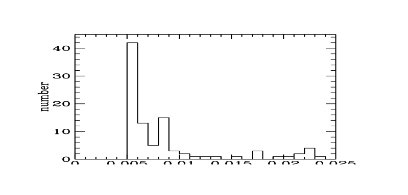
Figure 2: Plot illustrating the variable quality of the data. The histogram shows the distribution of measured values of the noise in the sky in the 96 reduced frame, in units of DN sec^-1. Taking into account read noise, dark noise, and Poisson noise from the counts in the sky, the expected noise is in the range $0.005-0.006$ DN sec^-1, corresponding to the peak in the histogram. As is evident, less than half the data lie within this range.

The next step was to use the data frames themselves to remove residuals, whether multiplicative (“flat field”) or additive (“sky subtraction”). To a first approximation the sky level is the same in all frames so that the residuals, from whatever cause, will be similar in each frame and can be removed by subtracting the median of the 96 frames. The step size between pointings, $3\arcsec$, was chosen to be sufficiently large that the quasar images from different frames would not overlap, so that objects would be successfully removed in taking the median. Subtracting the median of the 96 frames resulted in a very noticeable reduction in the noise in each frame. We understand that the explanation for this is that the frame used for dark subtraction has substantial read noise, so that noise is being added to each frame at the stage of dark subtraction. We remove this noise by subtracting the median frame. There is a new task which produces synthetic darks of low noise, which therefore avoids this problem. However we were advised by the NICMOS group at STScI that the procedure we followed produces equally satisfactory results.

At this stage we created a list of bad pixels by identifying discrepant high and low pixels in the median of the 96 frames, as well as pixels where the recorded values showed a large dispersion in the stack of 96 frames. The bad pixels were recorded as a “mask” frame for use at the stage of combining the six data frames from each field.

The quality of the NICMOS data is highly variable. First there are a few frames which contain an excessive number of cosmic ray hits. A related but more serious problem is a consequence of the passage of HST through the South Atlantic Anomaly (SAA) and the fact that these HgCdTe arrays suffer from remanence i.e. very high counts in a pixel are not completely flushed when the array is reset. Although the NICMOS cameras are switched off during passage through the SAA, the arrays experience a storm of cosmic-ray hits. In most cases the result of remanence of the cosmic-ray hits is a background with a very high noise level that affects subsequent images, and declines with time. The remanence images of individual cosmic-ray hits are usually difficult to discern, presumably indicating that the whole array has been hit. To quantify the effect on the data we measured the standard deviation in the counts in the background in each frame. Fig. 2 plots the histogram of these noise measurements. The peak in the histogram marks the noise in a clean frame, unaffected by the SAA. As shown in Fig. 2 in $20\%$ of our frames the noise is more than double that in an unadulterated frame and only about half the data are unaffected.

The NICMOS pipeline produces error frames which assume a Poisson noise model. For the majority of frames this will be inappropriate because of the additional source of noise discussed above. We therefore created our own noise frames by adding in quadrature the Poisson contribution from counts above sky to the measured noise in the background.

2.2.2 Mosaic combination

The pipeline task calnicb combines frames processed by calnica to produce a final mosaic image. We did not use calnicb because we wished to make a number of changes to the standard pipeline. The relatively poor quality of a significant fraction of the data demanded a more flexible approach that allowed each step in the combination process to be scrutinised. We were particularly concerned with identifying bad data, i.e. pixels with discrepant counts, either high or low, from whatever cause: for example due to cosmic rays not identified by calnica, or from transient variation of the quantum efficiency or dark current of any pixels. We used the routine driz_cr in the ditherII package (Fruchter and Hook 2000) to identify bad data. The first step was to align the six frames using integer pixel offsets, and to form the median, ignoring pixels in the bad-pixel mask. Each frame was then compared with the combination frame to identify discrepant data values. The bad pixels identified were combined with the original bad-pixel mask to form new individual masks for each frame. A defect in the form of horizontal bars is visible in some frames. These were identified and the pixels added to the respective masks. Using the new masks a revised combination frame was formed, and a revised identification of bad data was made.

The step size between pointings, $3\arcsec$, is by design an integer multiple of the pixel size, $0\aas@@fstack{\prime\prime}075$. The data frames were aligned to the nearest pixel, and then averaged, weighting by the inverse of the measured variance in the sky, and ignoring masked pixels. The associated error frame was also created as appropriate for the weighting and mask scheme used. We could have chosen sub-pixel dither steps and to drizzle the data (Fruchter and Hook 2000). We chose not to because the number of pointings is so small. In the event, in a few frames the step pattern executed produced residuals from the requested 40-pixel step of up to half a pixel. The sub-pixel residuals therefore broaden the psf very slightly. Fortunately the residuals were almost identical for each target, so the psfs of each quasar were affected in the same way.

The final frames are displayed in the left hand portion of Figs $5-8$ as $S/N$ maps i.e. the image frame divided by the error frame. Displayed in this way the reduced $S/N$ near the edges of the mosaic frames, where the number of overlapping frames is smaller, is evinced by the smaller number of sources visible on average in these regions. Over the regions where there are only two overlapping frames the data are of little value. This is because the scheme used to identify bad pixels is ineffective if the number of frames is less than three. In each of the pictures the bright point source below and to the right of the centre of the frame is the target quasar. In a number of cases objects are visible at small angular separations from the quasar. These are candidate counterparts of the DLA absorbers.

2.3 Psf subtraction

To identify candidates at small angular separation from the quasars, and to measure their properties, we need to subtract the images of the quasars. There are three possible methods for psf subtraction. We could use the Tiny Tim software to create artificial psfs, or we could use images of bright stars in the archive, or we could use the 15 quasar images themselves. The advantages of Tiny Tim psfs over real psfs are that the psfs are noiseless, and can be created at the required x, y location on the array (the psf varies with x, y location), and at the precise sub-pixel position (which is desirable as the psf is slightly undersampled). However because the accuracy of the Tiny Tim psfs is limited by the detail in the models, real psfs are preferred if suitably placed high $S/N$ images are available.

The main advantage of using images of bright stars is the high $S/N$, with the proviso that any non-linear behaviour of the detector must be accurately characterised. The undersampling of the psf nevertheless sets a fundamental limit to the accuracy achievable if a single star is used. Systematic residuals are unavoidable unless the star was positioned at exactly the same sub-pixel position as the target. Other disadvantages include possible poor colour match, and mismatch of the psf in terms of x, y location. Primarily to deal with the problem of undersampling we chose to use the 15 quasar images themselves to subtract the psfs. Because we have 15 targets we can use dithering to recover full sampling of the psf, without seriously compromising the $S/N$ of the composite psf. Additional advantages of using the quasars are that the colours are perfectly matched (assuming the range in colour is small), and that the initial x, y location and step pattern is the same for all the quasars. In addition all the observations were completed over a few months, so the condition of the telescope and camera was similar for each target. A drawback to this approach is that it diminishes the possibility of detecting the quasar host galaxies, since we will subtract the average host-galaxy profile from each image.

The procedure followed for each quasar was to create a subtraction psf by averaging the images of the other 14 quasars. Taking the relevant 14 images, the first step was to scale the images to the same count level, and to register them to the nearest half pixel. Then, using the dither package, the data were interlaced into pixels of side half the original size. This sub-pixelised psf was then scaled and registered to the quasar image by minimising $\chi^{2}$, computing the flux at the location of a pixel by interpolation. In computing the $\chi^{2}$, pixels within 0.3″of the quasar centroid were excluded from the sum. Having subtracted the images of all 15 quasars, mask frames were created by adding to the mask any galaxies found close to the quasar, as well as any remaining bad pixels visible. The whole procedure was then iterated, using the masks to exclude these pixels in creating the psfs, and in making the fits. In this second stage the quasar PHL 1222 was excluding from the averaging in creating subtraction psfs because of excess emission clearly visible. This excess emission is centred on the quasar and is likely to be from the host galaxy of the quasar.

Sub-pixelisation of the psf has two effects. First it improves the sampling and so reduces systematic errors in subtraction near the centre of the psf. However the resulting psf is noisier. Because of the limited number of quasars used the psf subtraction adds noise to the frames. This is more noticeable for the brightest quasars, since the subtraction psf is formed by scaling up the images of fainter quasars. The procedure could be improved, therefore, by using a sub-pixelised psf for subtraction near the centre of the quasar image, but using full-sized pixels away from the centre where the issue of sampling is less important.

The approach Kulkarni et al. (2000) followed was to use single bright stars for psf subtraction. They provide an extensive and detailed analysis of the sources of uncertainty using this approach. In section 3.2.3 we compare the accuracy of our psf subtraction with that of Kulkarni et al.

2.4 Calculation of error frames

Figure 3: Illustration of the rescaling of the Poisson errors to account for systematic errors associated with the psf subtraction. At each radius for each quasar the standard deviation $\sigma_{S/N}$ in the $S/N$ frame is measured. A function of the form $1.0+e^{-r/R}(a-b{\mathrm{H}_{AB}})$ is fit to the data. To plot all the data at once we apply the results of the fit to rescale the measured values to a specific radius $r=5$ pixels ($0.375\arcsec$) (left-hand plot), and a specific magnitude ${\mathrm{H}_{AB}=18.0}$ (right-hand plot). The left-hand plot then shows how the scaling increases for brighter quasars, and the right-hand plot shows how the scaling increases at smaller radii. The solid lines are the fitted function.

The final stage before searching for candidates was to compute revised $1\sigma$ error frames for each quasar. The purpose of this is to be able to measure the significance of candidate detections. The revised error frames must include the contribution of random and systematic errors associated with the psf subtraction. We first computed $S/N$ frames by dividing the subtracted frames by the current error frames. Ideally, if the subtraction psf were both noiseless, and perfectly accurate, then the distribution of counts in the $S/N$ frames, outside remaining objects, would be Gaussian with standard deviation $\sigma_{S/N}=1.0$. Because the subtraction psf is not noiseless, to account for the added noise we scaled the error frame by the measured $\sigma_{S/N}$ in the sky, and then created new $S/N$ frames. Even then $\sigma_{S/N}$, although now unity in the sky, increased towards the centre of the (subtracted) quasar. The increase was greater for the brighter quasars. The reason for this can be understood as follows. For bright objects, such as the quasars in this programme, the errors are dominated by object photon noise i.e. $\sqrt{N}$, where $N$ is the number of detected photons. Suppose that the psf has a fractional accuracy $f$ i.e. the typical residual for any pixel after psf subtraction is $fN$. Then in the $S/N$ frame the residuals will be visible as deviations of $S/N=f\sqrt{N}$, i.e. larger where the counts are larger, and larger for brighter quasars.

To quantify these systematic errors, for each quasar we measured $\sigma_{S/N}$ in annuli centred on the quasar, clipping out real objects. To these results we fit a function of the form $\sigma_{S/N}={\mathrm{m}ax}(1.0+e^{-r/R}(a-b{\mathrm{H}_{AB}}),1.0)$. The error frames were then rescaled by the fitted function. In this equation $r$ is the distance from the quasar centroid in pixels, $R$ is a scale length, $a$ and $b$ are constants, and ${\mathrm{H}_{AB}}$ is the apparent magnitude of the quasar. The fit of the function is illustrated in two plots in Fig. 3. These plots indicate that for quasars fainter than ${\mathrm{H}_{AB}}=18.5$ it is possible to achieve psf subtraction with negligible systematic error, but that the systematic errors increase rapidly at brighter magnitudes.

It is noticeable from the right hand plot in Fig. 3 that the scatter increases at smaller radii, so that the scaling becomes less reliable near the centre. From an inspection of the residuals for the different targets we judged that inside a radius of 4.5 pixels (0.34″) the psf subtraction is unreliable, and we set the data to zero inside this radius.

3 Detection of candidates, and catalogues

Figure 4: Plot of relation between ${\mathrm{H}_{AB}}$ aperture magnitude and impact parameter for the 41 candidate DLA galaxies, taken from Table 4. Solid symbols identify compact objects (C in Table 4), and open symbols diffuse objects (D in Table 4): circles mark candidates, triangles mark sources confirmed as the DLA counterpart. The curves mark the detection limits averaged for the 15 fields, solid for compact objects and dashed for diffuse sources. The vertical solid and dashed lines mark the inner radius limit used for the search for objects, for the small aperture (i.e. compact objects) and large aperture (i.e.diffuse objects) respectively. Candidates with centroids inside these limits are not considered reliable and have been excluded from the catalogue in Table 4.

3.1 Detection

In this subsection we describe the algorithm used to produce a list of candidates. We restricted the search to a box of side $7.5\arcsec$ centred on the quasar. A commonly used procedure for detecting sources is to convolve the frame with a filter, typically a Gaussian, and to identify peaks in the convolved frame. There were three reasons why we did not follow this approach. The first is that the noise in the subtracted frames is larger near the quasar centre, so we need a detection threshold that varies as the noise varies. The second is that objects with surface-brightness profiles very different from the filter profile will not be detected. So, for example, low-surface brightness galaxies could be missed. The third is that we wish to quote detection limits in a way such that it is possible easily to compute whether a hypothetical galaxy (of arbitrary shape, profile, and magnitude) would have been detected.

Our method is to convolve with detection filters in a manner that produces complete samples of objects that have $S/N$ above a specified threshold, as measured within circular apertures of specified sizes. The data and variance frames are convolved with circular top-hat filters, of size equal to the requested aperture. The frame formed by taking the ratio of the convolved data frame and the square root of the convolved variance frame contains, at each pixel, the summed $S/N$ within the aperture of any source centred at that pixel. This ratio frame is then searched for peaks above a chosen $S/N$ threshold.

We first ran a large-box median filter over the frames, and subtracted this off, to remove any remaining gradual variations in the background. We used two detection apertures, of diameter 6 pixels (0.45″) and 12 pixels (0.90″). The smaller aperture was designed to detect compact sources, and the larger aperture was designed to find objects of lower surface-brightness that had been missed by the first filter. The $S/N$ detection threshold was selected from a consideration of the distribution of the depths of negative peaks in the aperture $S/N$ frames. With the exception of one field there were no negative detections in any frame below $S/N=-6$ for either detection filter. For the quasar Q $2116-358$ the psf subtraction was less successful than for the other targets, and there are negative residuals at the position of two of the diffraction spikes with $S/N\sim-8$. With this in mind we set our detection threshold at $S/N=6$ with the expectation that nearly all the objects detected will be real, with the caveat that sources located on diffraction spikes will be less reliable. In fact with the exception of very red objects we expect that all real objects in our candidate list will be detected at higher $S/N$ in our STIS data. Therefore we will reassess the reliability of the candidate list on completion of the list of candidates detected in the STIS frames.

Inner radius limit. Because the psf subtraction inside $r=0.34\arcsec$ was judged unreliable (section 2.4) the inner radius to which objects can be detected is equal to the sum of 0.34″and the aperture radius. Therefore for the small aperture the inner radius limit is 0.56″, and for the large aperture the inner radius limit is 0.79″.

Detection limits. The candidate list, then, was constructed by identifying any peaks higher than 6.0 in the aperture $S/N$ frames. Real objects in the frames will be detected at higher $S/N$ with the filter that most closely matches the galaxy surface brightness profile. Therefore if a peak was found at the same location for both filters we eliminated the detection of lower $S/N$, and classified the object as compact (C) or diffuse (D) for detection with the small or large aperture filter respectively. At the location of each peak we integrated the counts within the aperture, and transformed this to an aperture ${\mathrm{H}_{AB}}$ magnitude using the photometry zero point provided in the file header (the data were calibrated by converting the count rates (DN/sec) to Jy by mulitplying by the factor $2.070\times 10^{-6}$). Then for each frame and for both filters we measured the average detection limit in annuli at several different radii. These values are listed In Table 3. In Fig. 4 we plot, for both filters, the radial profile of the detection limits averaged for the 15 fields. The average detection limit for compact (diffuse) sources is ${\mathrm{H}_{AB}}=25.0\,(24.4)$ at an angular separation of $0.56\arcsec\,(0.79\arcsec)$ from the quasar, improving to ${\mathrm{H}_{AB}}=25.5\,(24.8)$ at large angular separations.

Aperture magnitudes. All the magnitudes of the candidates (section 3.2) are quoted as aperture magnitudes i.e. we have simply summed the counts within the aperture and no aperture correction has been applied (aperture corrections are, nevertheless, discussed in section 3.2.1). We have not attempted to extrapolate to total magnitudes, since this would be unreliable for the faint sources. The use of aperture magnitudes makes it very simple to compute whether or not a hypothetical galaxy of specified surface brightness profile and impact parameter would have been detected in a particular field. One first computes the aperture magnitude of the galaxy, for the small and large apertures. For the hypothesised impact parameter one compares the two aperture magnitudes against the detection limits provided in Table 3 for the field in question. If the galaxy were brighter than either detection limit it would have been included in our catalogue.

Table 3: Aperture magnitude ${\mathrm{H}_{AB}}$ average detection limits as a function of impact parameter for each field, for compact and diffuse sources.

No.	Quasar	compact or	impact parameter (arcsec)
		diffuse	0.3	0.4	0.5	0.6	0.8	1.0	1.5	2.0	3.0
1	CS 73	C	23.77	24.34	24.94	25.21	25.44	25.58	25.71	25.72	25.74
		D	22.65	22.75	23.47	24.02	24.63	24.80	24.95	24.98	25.00
2	PC 0056+0125	C	23.89	24.44	24.95	25.16	25.37	25.48	25.59	25.62	25.63
		D	22.80	22.92	23.60	24.10	24.57	24.72	24.84	24.88	24.89
3	PHL 1222	C	23.51	24.08	24.74	25.08	25.39	25.59	25.75	25.78	25.79
		D	22.35	22.45	23.20	23.84	24.55	24.79	25.00	25.04	25.05
4	PKS 0201+113	C	25.33	25.56	25.71	25.76	25.78	25.80	25.81	25.81	25.81
		D	24.46	24.54	24.82	24.95	25.03	25.05	25.07	25.07	25.07
5	0216+0803	C	23.42	24.02	24.71	25.03	25.31	25.49	25.64	25.69	25.70
		D	22.23	22.34	23.13	23.75	24.48	24.71	24.89	24.94	24.96
6	PKS 0458$-$02	C	25.24	25.39	25.51	25.54	25.55	25.56	25.57	25.57	25.57
		D	24.36	24.45	24.66	24.75	24.80	24.80	24.82	24.83	24.83
7	PKS 0528$-$250	C	23.13	23.70	24.33	24.65	24.95	25.16	25.33	25.39	25.40
		D	21.97	22.07	22.81	23.41	24.12	24.37	24.59	24.64	24.66
8	H 0841+1256	C	23.81	24.20	24.61	24.78	24.98	25.10	25.21	25.24	25.25
		D	22.75	22.86	23.45	23.84	24.19	24.34	24.46	24.50	24.51
10	B2 1215+33	C	24.55	24.97	25.31	25.45	25.57	25.64	25.68	25.70	25.70
		D	23.48	23.58	24.16	24.52	24.80	24.88	24.93	24.95	24.96
11	Q 1223+1753	C	23.25	23.77	24.29	24.55	24.82	25.00	25.16	25.20	25.21
		D	22.15	22.26	22.94	23.47	24.00	24.21	24.41	24.46	24.47
12	H 1500$\#$13	C	25.27	25.49	25.65	25.69	25.70	25.71	25.72	25.72	25.72
		D	24.41	24.48	24.75	24.88	24.95	24.97	24.98	24.98	24.98
13	Q 2116$-$358	C	22.72	23.27	23.86	24.22	24.57	24.82	25.05	25.11	25.12
		D	21.46	21.56	22.40	22.97	23.72	24.01	24.31	24.36	24.38
14	Q 2206$-$1958	C	22.49	23.06	23.92	24.34	24.73	25.04	25.30	25.38	25.40
		D	21.23	21.34	22.10	22.89	23.87	24.21	24.55	24.63	24.65
15	BR 2212$-$1626	C	23.65	24.11	24.58	24.76	24.96	25.09	25.22	25.25	25.25
		D	22.61	22.71	23.36	23.77	24.17	24.33	24.46	24.50	24.51
16	2233.9+1318	C	24.02	24.56	25.14	25.39	25.60	25.73	25.83	25.85	25.86
		D	22.88	22.99	23.68	24.26	24.81	24.95	25.08	25.11	25.12

Table 4: Coordinates and aperture magnitudes of candidate DLA galaxies

Quasar	Quasar	Candidate	Right Ascension			Declination			${\mathrm{H}_{AB}}$	$S/N$	Offset	PA	Remarks
no.	name	no.	(J2000)						(aper)		″	∘ (E of N)
1	CS 73												no candidates
2	PC 0056+0125	N-2-1C	0	59	17.7082	1	42	06.684	25.33	8.3	2.32	62.1
		N-2-2C	0	59	17.7468	1	42	08.403	25.37	7.8	3.84	43.2
		N-2-3C	0	59	17.4756	1	42	09.344	24.51	16.8	3.97	-20.4
		N-2-4D	0	59	17.2594	1	42	04.345	21.51	123.3	4.78	-105.3
3	PHL 1222	N-3-1C	1	53	53.7802	5	02	56.764	23.86	33.5	1.81	-100.9
		N-3-2C	1	53	54.0429	5	02	59.652	21.24	248.6	3.32	39.8
		N-3-3D	1	53	53.6837	5	02	55.440	23.38	27.7	3.61	-117.4
4	PKS 0201+113	N-4-1C	2	03	46.8345	11	34	46.579	23.36	53.6	1.01	67.9
		N-4-2C	2	03	46.9602	11	34	45.318	24.75	16.2	2.90	107.4
		N-4-3C	2	03	46.7978	11	34	42.849	25.79	6.6	3.36	173.3
		N-4-4C	2	03	46.8794	11	34	42.548	24.88	14.2	3.96	156.5
5	0216+0803	N-5-1C	2	18	57.2276	8	17	27.443	25.75	6.3	1.41	-104.8	Note 1
		N-5-2D	2	18	57.5773	8	17	27.264	24.34	10.5	3.82	97.8
6	PKS 0458$-$02	N-6-1D	5	01	12.6411	-1	59	14.711	24.60	7.6	0.86	-160.8
		N-6-2D	5	01	12.6940	-1	59	15.502	24.49	8.1	1.67	162.5
		N-6-3C	5	01	12.5480	-1	59	16.177	24.93	11.6	2.82	-143.8
		N-6-4C	5	01	12.8168	-1	59	12.045	24.96	11.5	2.98	51.5
		N-6-5C	5	01	12.8944	-1	59	11.610	24.29	19.9	4.17	56.7
7	PKS 0528$-$250	N-7-1C	5	30	07.9705	-25	03	31.170	25.54	5.0	1.14	159.0	Note 2
		N-7-2D	5	30	08.0753	-25	03	33.271	24.63	6.3	3.65	150.1
8	H 0841+1256	N-8-1C	8	44	24.2166	12	45	47.182	22.52	64.6	1.08	-80.6
		N-8-2C	8	44	24.4526	12	45	48.413	25.20	6.7	2.76	59.3
		N-8-3D	8	44	24.3525	12	45	43.156	22.73	30.7	3.91	166.8
10	B2 1215+33	N-10-1C	12	17	32.5264	33	05	36.052	25.75	6.3	2.03	-178.5
		N-10-2D	12	17	32.4597	33	05	34.975	23.71	18.6	3.23	-164.0
11	Q 1223+1753												no candidates
12	H 1500$\#$13	N-12-1D	14	54	18.4720	12	10	50.759	25.04	6.2	3.89	-162.8
13	Q 2116$-$358	N-13-1D	21	19	27.4733	-35	37	41.641	23.94	8.1	1.36	-109.0	Note 1
		N-13-2C	21	19	27.5516	-35	37	45.003	23.46	27.7	3.80	-174.6
		N-13-3C	21	19	27.9659	-35	37	39.795	23.51	27.0	4.87	73.1
14	Q 2206$-$1958	N-14-1C	22	08	52.1019	-19	43	58.456	25.11	6.5	1.13	23.6	Notes 1, 3
		N-14-2C	22	08	52.0480	-19	43	58.192	24.53	12.1	1.33	-13.2
		N-14-3C	22	08	52.1966	-19	43	58.213	25.27	7.2	2.20	54.3
		N-14-4C	22	08	51.8986	-19	43	59.055	25.11	7.8	2.44	-79.9
		N-14-5D	22	08	52.2106	-19	44	02.484	24.64	6.3	3.54	146.3
15	BR 2212$-$1626	N-15-1D	22	15	27.3782	-16	11	32.611	24.31	6.7	1.14	100.4
		N-15-2C	22	15	27.1966	-16	11	32.784	21.22	207.5	1.53	-104.7
		N-15-3C	22	15	27.3681	-16	11	34.450	22.99	47.5	2.25	154.6
		N-15-4C	22	15	27.5349	-16	11	32.041	25.14	7.0	3.38	83.7
		N-15-5C	22	15	27.1766	-16	11	29.211	25.37	6.2	3.61	-29.0
16	2233.9+1318	N-16-1D	22	36	19.2800	13	26	18.405	25.05	6.6	2.78	158.6	Note 4
		N-16-2C	22	36	19.4239	13	26	22.236	25.12	12.2	3.32	68.3

1. The three sources N-5-1C, N-13-1D, and N-14-1C lie on diffraction spikes and should therefore be considered less certain/reliable than the other sources.

2. This source is the DLA at $z=2.8110$ confirmed by Møller and Warren (1993), and so has been included even though it has $S/N<6$.

3. This source has been confirmed by us as the DLA at $z=1.9205$ (Møller et al, in preparation).

4. This source is the LLS at $z=3.1501$ confirmed by Djorgovski et al. (1996).

3.2 Catalogue

The catalogue of detections is provided in Table 4. For each quasar field the candidates are listed in order of angular separation from the quasar. Listed in the first three columns of Table 4 are the quasar number, quasar name, and the candidate number. The candidate numbering scheme is explained as follows. Taking as example candidate N-15-3C, the ‘N’ stands for NICMOS (we will provide a similar list ‘S’ for the STIS images), 15 is the quasar number, the 3 indicates that it is the third nearest candidate to the quasar in that field, and the C states that it is compact. We find a total of 41 candidates. The magnitudes and impact parameters are compared against the average detection limits in Fig. 4. The positions of the candidates are illustrated in the finding charts in the right-hand panels in Figs $5-8$. The remaining columns in Table 4 list successively the coordinates, aperture magnitude, detection $S/N$, angular separation from the quasar, and the position angle from the quasar. The NICMOS data header files contain an astrometric solution that provides coordinates that are accurate in a relative sense, for the small angular separations with which we are concerned. The coordinates were shifted to absolute values by adopting for the coordinates of the quasar the value measured from the DSS plate, listed in Table 2.

Table 5: Sersic profile fits to brighter candidates

No.	Quasar	Candidate	$r_{e}$	$n$	orient’n	ellip	${\mathrm{H}_{AB}}$	${\mathrm{\Delta}H_{AB}}$	comments
			$\arcsec$		∘ (E of N)		(total)	(ap. corr.)
2	PC 0056+0125	N-2-4D	$0.212^{+0.008}_{-0.008}$	$2.57^{+0.15}_{-0.14}$	$64.4^{+0.5}_{-0.5}$	$0.70^{+0.01}_{-0.01}$	21.06	0.45
3	PHL 1222	N-3-1C	$0.119^{+0.006}_{-0.006}$	$0.65^{+0.17}_{-0.16}$	$-27.1^{+...}_{-...}$	$0.05^{+0.09}_{-...}$	23.35	0.51	Note 1
		N-3-2C							point source (Q 0151+0448B)
		N-3-3D	$0.437^{+0.053}_{-0.035}$	$0.84^{+0.21}_{-0.16}$	$-27.2^{+11.5}_{-10.6}$	$0.21^{+0.07}_{-0.07}$	22.54	0.84	faint companions masked
4	PKS 0201+113	N-4-1C	$0.203^{+0.011}_{-0.009}$	$1.21^{+0.15}_{-0.13}$	$-1.9^{+3.0}_{-3.0}$	$0.38^{+0.03}_{-0.03}$	22.40	0.96
6	PKS 0458$-$02	N-6-5C	$0.103^{+0.008}_{-0.008}$	$0.41^{+0.25}_{-0.19}$	$53.0^{+4.5}_{-4.5}$	$0.60^{+0.06}_{-0.07}$	23.79	0.50
8	H 0841+1256	N-8-1C	$0.068^{+0.005}_{-0.005}$	$2.69^{+0.50}_{-0.40}$	$-53.1^{+1.7}_{-1.7}$	$0.70^{+0.03}_{-0.03}$	21.95	0.57
		N-8-3D	$0.371^{+0.018}_{-0.015}$	$0.61^{+0.12}_{-0.10}$	$-78.8^{+5.1}_{-4.9}$	$0.34^{+0.04}_{-0.05}$	22.11	0.62
10	B2 1215+33	N-10-2D	$0.256^{+0.035}_{-0.024}$	$0.93^{+0.36}_{-0.25}$	$72.4^{+2.5}_{-2.6}$	$0.73^{+0.04}_{-0.04}$	23.21	0.50
13	Q 2116$-$358	N-13-2C	$0.130^{+0.026}_{-0.016}$	$2.23^{+0.82}_{-0.54}$	$-86.0^{+13.4}_{-12.8}$	$0.28^{+0.09}_{-0.10}$	22.74	0.72
		N-13-3C	$0.170^{+0.010}_{-0.009}$	$0.65^{+0.20}_{-0.16}$	$-29.7^{+9.0}_{-8.9}$	$0.28^{+0.07}_{-0.08}$	22.74	0.77
15	BR 2212$-$1626	N-15-2C							point source
		N-15-3C	$0.115^{+0.006}_{-0.006}$	$1.28^{+0.22}_{-0.19}$	$89.3^{+2.9}_{-2.9}$	$0.50^{+0.04}_{-0.04}$	22.37	0.62

1. This source is almost round. In consequence the confidence limits on the orientation are indeterminate, as is the lower confidence limit for the ellipticity.

3.2.1 Surface-brightness profiles

For the brighter candidates we have measured the deconvolved surface brightness profile using the techniques described by Warren et al (1996). We use the Sersic model where the surface brightness as a function of radius $r$ is $\Sigma=\Sigma_{e}\exp\{-B(n)[(r/r_{e})^{1/n}-1]\}$. The parameter $n$ characterises the shape of the profile: $n=1$ is the exponential profile and $n=4$ the de Vaucouleurs profile. This parameterisation is particularly useful, therefore, as the value of $n$ can be used to classify faint galaxies into “early” and “late” types. The parameter $r_{e}$ is the half-light radius, $\Sigma_{e}$ is the surface brightness at the half-light radius, and $B(n)$ is a constant for particular $n$. Ciotti and Bertin (1999) provide the series asymptotic solution for $B(n)$, and we used the approximation provided by the first four terms $B(n)=2n-1/3+4/(405n)+46/(25515n^{2})$ which is accurate to better than one part in $10^{6}$ over the range of $n$ of interest.

We created a psf using the Tiny Tim software, with pixels one-third the size of the NIC2 pixels, to ensure adequate sampling. The fitting proceeds by creating a two-dimensional galaxy surface-brightness profile with the same small pixel size, convolving with the psf, rebinning to the full pixel size and computing the $\chi^{2}$ of the fit. The best fit is found by $\chi^{2}$ minimisation on the seven parameters $x$, $y$, $\Sigma_{e}$, $r_{e}$, $n$, orientation, and ellipticity. In Table 5 we provide the details of the fits to all the candidates in Table 4 with $S/N>18$. Also listed there are the total magnitudes, computed by extrapolating the models to infinite radius, and the aperture corrections i.e. the difference between the total and aperture magnitudes. It is of interest to compare the aperture corrections for these galaxies with the values for a point source. For a point source the aperture correction for the small aperture (used for compact objects) is 0.444 mag. Excluding the two point sources listed in Table 5, there are seven compact objects, for which the mean aperture correction is 0.66 mag., with a scatter of 0.16 mag. For a point source the aperture correction for the large aperture (used for diffuse objects) is 0.134 mag. There are four diffuse objects listed in Table 5, for which the mean aperture correction is $0.60\pm 0.17$ mag.

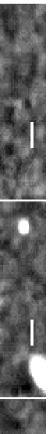
Figure 5: N.B. This is not the full resolution figure which is available at astro.ic.ac.uk/Research/extragal/dla.html. Reduced frames showing the images of four of the targets before and after psf subtraction. The pixel size is $0\aas@@fstack{\prime\prime}075$. The targets are, from top to bottom, nos 1. CS 73, 2. PC 0056+0125, 3. PHL 1222, 4. PKS 0201+113. In each case the left image is the pixel $S/N$ frame formed by dividing the data frame by the error frame, and shows the full mosaic field $25\aas@@fstack{\prime\prime}0\times 22\aas@@fstack{\prime\prime}2$. The compass points N with the arm to the E. The length of the arm is $3\arcsec$. The central image is a $\times 3$ zoom of the $7\aas@@fstack{\prime\prime}5\times 7\aas@@fstack{\prime\prime}5$ region centred on the target, after psf subtraction. The vertical bar is of length $1\arcsec$. This shows the $S/N$ frame for the small detection filter i.e. the $S/N$ within an aperture of diameter 0.45″centred at that point. Peaks above $S/N=6$ are compact candidates. To detect diffuse candidates a corresponding frame for an aperture of diameter 0.9″was constructed. The right-hand frame identifies the candidates, listed in Table 4. The symbol size scales with brightness. Filled symbols are compact candidates, open symbols diffuse. Brighter objects are plotted at the correct deconvolved orientation and ellipticity (Table 5), while fainter sources are plotted as circles. The cross marks the quasar position.

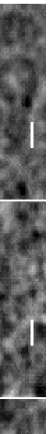
Figure 6: N.B. This is not the full resolution figure which is available at astro.ic.ac.uk/Research/extragal/dla.html. Reduced frames showing the images of four of the targets before and after psf subtraction. The pixel size is $0\aas@@fstack{\prime\prime}075$. The targets are, from top to bottom, nos 5. 0216+0803, 6. PKS 0458$-$02, 7. PKS 0528$-$250, 8. H 0841+1256. In each case the left image is the pixel $S/N$ frame formed by dividing the data frame by the error frame, and shows the full mosaic field $25\aas@@fstack{\prime\prime}0\times 22\aas@@fstack{\prime\prime}2$. The compass points N with the arm to the E. The length of the arm is $3\arcsec$. The central image is a $\times 3$ zoom of the $7\aas@@fstack{\prime\prime}5\times 7\aas@@fstack{\prime\prime}5$ region centred on the target, after psf subtraction. The vertical bar is of length $1\arcsec$. This shows the $S/N$ frame for the small detection filter i.e. the $S/N$ within an aperture of diameter 0.45″centred at that point. Peaks above $S/N=6$ are compact candidates. To detect diffuse candidates a corresponding frame for an aperture of diameter 0.9″was constructed. The right-hand frame identifies the candidates, listed in Table 4. The symbol size scales with brightness. Filled symbols are compact candidates, open symbols diffuse. Brighter objects are plotted at the correct deconvolved orientation and ellipticity (Table 5), while fainter sources are plotted as circles. The cross marks the quasar position.

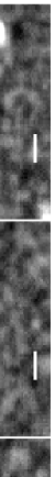
Figure 7: N.B. This is not the full resolution figure which is available at astro.ic.ac.uk/Research/extragal/dla.html. Reduced frames showing the images of four of the targets before and after psf subtraction. The pixel size is $0\aas@@fstack{\prime\prime}075$. The targets are, from top to bottom, nos 10. B2 1215+33, 11. Q 1223+1753, 12. H 1500$\#$13, 13. Q 2116$-$358. In each case the left image is the pixel $S/N$ frame formed by dividing the data frame by the error frame, and shows the full mosaic field $25\aas@@fstack{\prime\prime}0\times 22\aas@@fstack{\prime\prime}2$. The compass points N with the arm to the E. The length of the arm is $3\arcsec$. The central image is a $\times 3$ zoom of the $7\aas@@fstack{\prime\prime}5\times 7\aas@@fstack{\prime\prime}5$ region centred on the target, after psf subtraction. The vertical bar is of length $1\arcsec$. This shows the $S/N$ frame for the small detection filter i.e. the $S/N$ within an aperture of diameter 0.45 ″centred at that point. Peaks above $S/N=6$ are compact candidates. To detect diffuse candidates a corresponding frame for an aperture of diameter 0.9″was constructed. The right-hand frame identifies the candidates, listed in Table 4. The symbol size scales with brightness. Filled symbols are compact candidates, open symbols diffuse. Brighter objects are plotted yat the correct deconvolved orientation and ellipticity (Table 5), while fainter sources are plotted as circles. The cross marks the quasar position.

Figure 8: N.B. This is not the full resolution figure which is available at astro.ic.ac.uk/Research/extragal/dla.html. Reduced frames showing the images of three of the targets before and after psf subtraction. The pixel size is $0\aas@@fstack{\prime\prime}075$. The targets are, from top to bottom, nos 14. Q 2206$-$1958, 15. BR 2212$-$1626, 16. 2233.9+1318. In each case the left image is the pixel $S/N$ frame formed by dividing the data frame by the error frame, and shows the full mosaic field $25\aas@@fstack{\prime\prime}0\times 22\aas@@fstack{\prime\prime}2$. The compass points N with the arm to the E. The length of the arm is $3\arcsec$. The central image is a $\times 3$ zoom of the $7\aas@@fstack{\prime\prime}5\times 7\aas@@fstack{\prime\prime}5$ region centred on the target, after psf subtraction. The vertical bar is of length $1\arcsec$. This shows the $S/N$ frame for the small detection filter i.e. the $S/N$ within an aperture of diameter 0.45″centred at that point. Peaks above $S/N=6$ are compact candidates. To detect diffuse candidates a corresponding frame for an aperture of diameter 0.9″was constructed. The right-hand frame identifies the candidates, listed in Table 4. The symbol size scales with brightness. Filled symbols are compact candidates, open symbols diffuse. Brighter objects are plotted at the correct deconvolved orientation and ellipticity (Table 5), while fainter sources are plotted as circles. The cross marks the quasar position.

3.2.2 Results

We now comment on the results for the individual fields in turn.

1. CS 73, Fig. 5. The spectrum of this source shows a LLS at $z=1.8862$ and a DLA at $z=2.0713$ (Table 1), but no candidate counterparts were found in this field.

2. PC 0056+0125, Fig. 5. There is a strong DLA line at $z=2.7771$ in the spectrum of this quasar. Bearing in mind the small impact parameters of the few confirmed DLA counterparts we consider the nearest candidate, N-2-1C which lies at an angular separation of 2.32″, to be the most likely of the four candidate counterparts listed in Table 4. The large ellipticity, 0.70, of the candidate N-2-4D suggests that this is a late-type galaxy viewed at a high inclination angle. The orientation of the image is only 10^∘ from the line joining the quasar to the galaxy. Therefore a possible alternative explanation of the DLA line is the presence of an extended gaseous disk around this galaxy.

3. PHL 1222, Fig. 5. The redshift of the DLA $z=1.9342$ is close to the redshift of the quasar $z=1.922$. The DLA absorbs much of the quasar Ly$\alpha\,$emission line, and to measure the column density it was necessary to model the unabsorbed Ly$\alpha\,$emission line profile (Møller et al 1998). There are significant residuals visible after the psf subtraction, which are approximately circularly symmetric, which we suggest are most likely to be due to the quasar host galaxy. The DLA absorber has been detected in Ly$\alpha\,$emission by Fynbo et al. as an extended object 6 arcsec across, centred 0.9″E of the quasar. These authors suggest that the source of ionising photons is the nearby quasar Q 0151+0448B, rather than young stars. This quasar lies at an angular separation of 3.32″, and is listed in Table 4 as source N-3-2C. We do not find a source coincident with the centre of the Ly$\alpha\,$emission, consistent with the photoionisation explanation.

4. PKS 0201+113, Fig. 5. The spectrum of this source shows a DLA absorber at $z=3.3875$. There is a relatively bright compact source N-4-1C with ${\mathrm{H}_{AB}=23.36}$ only 1.01″from the quasar, which is a good candidate for the counterpart. This object has $n=1.21$ i.e. the surface-brightness profile approximates an exponential.

5. 0216+0803, Fig. 6. The spectrum of this source shows a confirmed DLA absorber at $z=2.2930$. There is also a high-column density system at $z=1.7688$ confirmed as such by Lu et al. (1996) on the basis of the detection of the weak metal lines of Fe II $\lambda$2260, Mn II $\lambda$2576, and Ni II $\lambda$1751. The value for the HI column density however comes from the the Ly$\alpha\,$line equivalent width measured by Lanzetta et al (1991) from a low resolution spectrum, and is therefore uncertain. The nearest candidate counterpart N-5-1C lies at an angular separation of 1.41″. As noted in Table 4 this object lies on a diffraction spike, and therefore should be considered less reliable than other sources, especially given the relatively low $S/N$ of 6.3.

6. PKS 0458$-$02, Fig. 6. This quasar shows extended radio emission. Analysis of the 21 cm line in absorption allowed Briggs et al (1989) to place a lower limit on the size of the DLA absorber ($z=2.0395$) of $8h^{-1}$ kpc. The nearest candidate counterpart is the faint ${\mathrm{H}_{AB}=24.60}$ diffuse object N-6-1D, at an angular separation of only 0.86 arcsec. This candidate is the closest to the quasar of all the candidates listed in Table 4, and very close to our inner radius limit of 0.79 arcsec for the detection of diffuse objects. The object does not stand out clearly in Fig. 6 (middle column) as this is the detection frame for compact objects. We see no reason to doubt the reality of this object. The source N-6-3C lies on the diffraction spike of a nearby bright star, and the measured magnitude will overestimate the brightness of this source.

7. PKS 0528$-$250, Fig. 6. There are two DLA absorbers in the spectrum of this quasar at $z=2.1408$ and $z=2.8110$. The galaxy counterpart of the higher redshift system was discovered by Møller and Warren (1993) and has been extensively studied (Warren and Møller 1996, Møller and Warren 1998). This source is detected in our NICMOS image at $S/N=5.0$, and we have included the object in Table 4 even though it is fainter than the detection limit $S/N=6$. The STIS image of the source is presented in Møller et al (in preparation). The $z=2.8110$ DLA system absorbs the quasar Ly$\alpha\,$emission line. The column density quoted for this absorber in Table 1 is taken from Møller and Warren (1993) who attempted to account for the quasar Ly$\alpha\,$emission in making the fit (in the same manner as with PHL 1222).

8. H 0841+1256, Fig. 6. The redshift of H 0841+1256 is uncertain. The object was discovered by Hazard in a search of an objective prism plate, and may be a BL Lac as no emission lines have been detected. The redshift is estimated from the wavelength of the onset of absorption in the Ly$\alpha\,$forest, but this cannot be measured accurately as it coincides with the wavelength of the $z=2.4764$ DLA absorber, which also absorbs any Ly$\alpha\,$emission that might be present. There are two confirmed DLA absorbers in the spectrum of this object, at $z=2.3745$ and $z=2.4764$. A candidate DLA absorption line near 3480Å  remains to be confirmed.

The source N-8-1C was first detected by Aragón-Salamanca, Ellis, and O’Brien (1996) in a K-band image obtained at the United Kingdom Infrared Telescope (UKIRT). They measured ${\mathrm{K}=19.9}$ (Johnson) for this source. Taking the total magnitude from Table 5 and converting to the Johnson system, our measurement gives ${\mathrm{H}=20.7}$, and a colour ${\mathrm{H}-K=0.8}$.

9. PC 0953+4749. As stated earlier the NICMOS observations of this source failed. The redshifts and column densities of the three DLA absorbers were measured from a spectrum taken with the Keck I telescope. The spectrum will be presented in Bunker et al. (in preparation) together with WFPC2 observations of the field.

10. B2 1215+33, Fig. 7. There is a single DLA absorber at $z=1.9990$ in the spectrum of this quasar. This field was also observed by Aragón-Salamanca et al (1996) who report the detection of a candidate with ${\mathrm{K}=20.1}$ (Johnson) located $1.3\arcsec$ E of the quasar. This candidate therefore is 0.2 mag fainter in K than N-8-1C. However N-8-1C has an aperture magnitude of ${\mathrm{H}_{AB}=22.5}$ whereas we do not detect their fainter candidate above our detection thresholds of ${\mathrm{H}_{AB}=25.7}$ and 24.9 for compact and diffuse sources respectively. If the object had a similar colour and surface brightness profile to N-8-1C we would have expected to find a compact source with an aperture magnitude of ${\mathrm{H}_{AB}=22.7}$. This implies that their candidate, if real, is exceptionally red.

11. Q 1223+1753, Fig. 7. There is a single DLA absorber at $z=2.4658$ in the spectrum of this quasar, but no candidate counterparts have been detected. Several of the images of this field suffer from high background noise (§2.2.1).

12. H 1500$\#$13, Fig. 7. There is a DLA absorber at $z=3.1714$ seen in the spectrum of this source. After psf subtraction a strong residual to the SW and close to the quasar remains, which is clearly visible in Fig. 7. The centroid of the residuals lies inside our detection radius limit, and the tangential orientation of the residual leads us to believe that it is not due to a galaxy counterpart of the absorber, but could possibly be emission from the quasar host galaxy.

13. Q 2116$-$358, Fig. 7. The spectrum of this quasar shows a LLS absorption line at $z=1.9966$. This is the second brightest quasar in our list. The psf subtraction for this quasar is particularly poor, leading to strong negative residuals for two of the diffraction spikes. This is the only object for which such a pattern of residuals is seen, suggesting that the observing configuration was different in some way. Although we have been unable to identify a cause we note that this quasar was the first to be observed in our campaign. A ring of excess emission is seen in Fig. 7 which could be due to the host galaxy of the quasar. The candidate source closest to the quasar lies on a diffraction spike and therefore should be considered less reliable than other sources.

14. Q 2206$-$1958, Fig. 8. The nearest source to the quasar N-14-1C, which lies at an offset of 1.13″, has been confirmed by us as the counterpart to the DLA absorber at $z=1.9205$ (Møller et al., in preparation). The source lies on a diffraction spike. The psf subtraction for this source is comparatively poor, so the uncertainty on the magnitude is larger than that indicated by the $S/N$ quoted in Table 4. The spectrum of this quasar shows a second DLA absorber at $z=2.0762$.

15. BR 2212$-$1626, Fig. 8. There is a LLS absorber at $z=3.6617$ in the spectrum of this quasar. There are two relatively bright candidates in this field. With FORS on the VLT we have obtained a spectrum of the brightest source N-15-2C, which lies at an angular separation of 1.53″. This spectrum shows that the candidate source is a quasar at the same redshift as BR 2212$-$1626 (the spectrum will be presented in a future paper describing spectroscopy of our NICMOS and STIS candidates). While the hypothesis requires further investigation at present we consider it unlikely that this is a gravitational lens system, as we see no sign of a lensing galaxy in our NICMOS image.

16. 2233.9+1318, Fig. 8. The faint diffuse source N-16-1D with ${\mathrm{H}_{AB}=25.05}$ is the counterpart of the LLS at $z=3.1501$. This object was first detected, and proposed as the couterpart, by Steidel, Pettini, and Hamilton (1995), who measured an offset from the quasar of $2.9\arcsec$, in agreement with our value of $2.78\arcsec$. The object was discovered independently by Djorgovski et al (1996), who confirmed the identification through the spectroscopic detection of Ly$\alpha\,$emission. They quote a smaller offset of $2.3\arcsec$. This object has also been detected in our STIS image (Møller et al, in preparation). As with the quasar H1500$\#$13 after psf subtraction there is residual emission close to the quasar, inside our detection radius limit, which we do not believe is associated with the absorber.

3.2.3 Comparison with other work

Kulkarni et al. (2000) observed the quasar LBQS 1210+1731 with the NIC2 camera and F160W filter for a single orbit (2560 sec integration time), and detected a candidate DLA absorber counterpart at an impact parameter of $0.25\arcsec$, at $4.1\sigma$ significance. The object is compact and would have an aperture magnitude of ${\mathrm{H}_{AB}=21.87}$. This object is rather bright. Placing it in Fig. 4 it can be seen that it is more than three magnitudes brighter than the three spectroscopcially confirmed DLA galaxy counterparts (${\mathrm{H}_{AB}=25.05,25.11,25.54}$), indicated by triangles.

As seen in Fig. 4, our average detection limit becomes rapidly brighter at small impact parameters. Nevertheless their object lies well above our $6\sigma$ detection limits. Our average limit for compact objects at $0.3\arcsec$ is ${\mathrm{H}_{AB}=23.87}$, with range 22.49 to 25.33 (Table 3), so we would easily have detected a similar object in any of our frames. Indeed we do find a few bright candidates at small impact parameters. However we have chosen, conservatively, not to list candidates inside $0.56\arcsec$ for the reasons set out in section 2.4.

The accuracy of psf subtraction of the two methods appears to be comparable. We compute an equivalent detection limit for their data of ${\mathrm{H}_{AB}=22.12}$, by scaling their measured noise at $0.3\arcsec$ ($0.28\mu$Jy per pixel) to our longer integration time. Their quasar has ${\mathrm{H}_{AB}=16.95\pm 0.05}$ (total, P Hewett, private communication), similar in brightness to our two brightest targets, quasars 13 and 14. Our detection limits for these quasars are 22.72 and 22.49.

3.3 Summary

In this paper we have described a search for the galaxy counterparts of 23 high-redshift high-column density Ly$\alpha$ absorbers seen in the spectra of 16 quasars, using the HST NICMOS instrument. Within a box of side $7.5\arcsec$ centred on each quasar, over all the fields we have found a total of 41 candidates, of which 3 have already been confirmed spectroscopically as the counterparts. We provide detection limits as a function of impact parameter for each field, and the use of aperture magnitudes makes it very simple to compute whether a hypothetical galaxy of specified luminosity profile and impact parameter would have been detected in our survey. Our aperture-magnitude detection limits ${\mathrm{H}_{AB}\sim 25}$, the small minimum impact parameter $0.56\arcsec$, and the sample size make this the most sensitive search yet made for the galaxies producing high-redshift DLA absorption lines. At the same time we are obtaining very-deep optical images using STIS, which will provide an additional list of candidates (Møller et al., in preparation). Except for unusually red galaxies the STIS images will reach substantially deeper than the NICMOS images, and therefore can be used to check the reliability of the candidate list provided in Table 4. A discussion of the conclusions that may be drawn from the imaging data, and the limited spectroscopic follow-up so far completed, is deferred to the STIS paper.

The next stage of this programme is a campaign of spectroscopy to measure the redshifts of the candidates, to identify which are counterparts of the absorbers. Since the galaxies are mostly faint, and close to the quasar, redshift determination will be difficult. The best hope will be to detect Ly$\alpha$ emission. Although this line is readily extinguished by dust, and therefore may be weak, it is likely to be the easiest to detect because at this wavelength the light from the quasar is removed by the absorber itself.

References

- [1996] Aragón-Salamanca A., Ellis R. S., O’Brien K. S., 1996, MNRAS 281, 945
- [1989] Briggs F. H., Wolfe A. M., Liszt H. S., Davis M. M., Turner K. L., 1989, ApJ 341, 650
- [1999] Bunker A. J., Warren S. J., Clements D. L., Williger G. M., Hewett P. C., 1999, MNRAS 309, 875
- [1999] Ciotti L., Bertin G., 1999, A&A 352, 447
- [1996] Djorgovski S. G., Pahre M. A., Bechtold J., Elston R., 1996, Nature 382, 234
- [1999] Fynbo J. U., Møller P., Warren S. J., 1999, MNRAS 305, 849
- [1997] Haehnelt M. G., Steinmetz M., Rauch M., 1998, ApJ 495, 647
- [1997] Fruchter A. S., Hook R. N., 2000, PASP, submitted
- [2000] Kulkarni V. P., Hill J. M., Schneider G., Weymann R. J., Storrie-Lombardi L. J., Rieke M. J., Thompson R. I., Jannuzi B. T., 2000, ApJ in press
- [1991] Lanzetta K. M., Wolfe A. M., Turnshek D. A., Lu L., Mc Mahon R. G., Hazard C., 1991, ApJS 77, 1
- [1997] Le Brun V., Bergeron J., Boissé P., Deharveng J. M., 1997, A&A 321, 733
- [1998] Ledoux C., Petitjean P., Bergeron J., Wampler E. J., Srianand R., 1998, A&A 337, 51
- [1997] Lu L., Sargent W. L. W., Barlow T. A., Churchill C. W., Vogt S. S., 1996, ApJS 107, 475
- [1994] Lu L., Wolfe A. M., 1994, AJ 108, 44
- [1993] Lu L., Wolfe A. M., Turnshek D. A., Lanzetta K. M., 1993, ApJS 84, 1
- [1994] Møller P., Jakobsen P., Perryman M. A. C., 1994, A&A 287, 719
- [1993] Møller P., Warren S. J., 1993, A&A 270, 43
- [1996] Møller P., Warren S. J., 1998, MNRAS 299, 661
- [1996] Møller P., Warren S. J., Fynbo J. U., 1998, A&A 330, 19
- [1993] Morton D. C., Chen J., Wright A. E., Peterson B. A., Jauncey D. L., 1980, MNRAS 193, 399
- [1999] Pei Y. C., Fall S. M., Hauser M. G., 1999, ApJ 522, 604
- [1994] Pettini M., Smith L. J., Hunstead R. W., King D. L., 1994, ApJ 426, 79
- [1997] Pettini M., Smith L. J., King D. L., Hunstead R. W., 1997, ApJ 486, 665
- [1997] Prochaska J. X., Wolfe A. M., 1997, ApJ 474, 140
- [1991] Schneider D. P., Schmidt M, Gunn J. E., 1991, AJ, 101, 2004
- [1995] Steidel C. C., Pettini M., Hamilton D., 1995, AJ 110, 2519
- [1998] Véron-Cetty M.-P., Véron P., 1998, ESO Scientific Report No. 18
- [1996] Warren S. J., Møller P., 1996, A&A 311, 25
- [1996] Warren S. J., Hewett P. C., Lewis G. F., Møller P., Iovino A., Shaver P. A., 1996, MNRAS 278, 139
- [1993] White R. L., Kinney A. L., Becker R. H., 1993, ApJ 407, 456
- [1987] Wolfe A. M., Turnshek D. A., Smith H. E., Cohen R. D., 1986, ApJS 61, 249
- [1995] Wolfe A. M., Lanzetta K. M., Foltz C. B., Chaffee F. H., 1995, ApJ 454, 698