Mayall II $\equiv$ G1 in M31:
Giant Globular Cluster or Core of a Dwarf Elliptical Galaxy? ^1,2

Abstract

Mayall II $\equiv$ G1 is one of the brightest globular clusters belonging to M31, the Andromeda galaxy. Our observations with the Wide Field and Planetary camera WFPC2 onboard the Hubble Space Telescope (HST) provide photometric data for the $I$ vs. $V-I$ and $V$ vs. $V-I$ color-magnitude diagrams. They reach stars with magnitudes fainter than $V$ = 27 mag, with a well populated red horizontal branch at about $V$ = 25.3 mag.

From model fitting, we determine a rather high mean metallicity of [Fe/H] = –0.95 $\pm$ 0.09, somewhat similar to 47 Tucanae. In order to determine our true measurement errors, we have carried out artificial star experiments. We find a larger spread in $V-I$ than can be explained by the measurement errors, and we attribute this to an intrinsic metallicity dispersion amongst the stars of G1; this may be the consequence of self-enrichment during the early stellar/dynamical evolutionary phases of this cluster. So far, only $\omega$ Centauri, the giant Galactic globular cluster, has been known to exhibit such an intrinsic metallicity dispersion, a phenomenon certainly related to the the deep potential wells of these two star clusters.

We determine, from the same HST/WFPC2 data, the structural parameters of G1. Its surface brightness profile provides its core radius $r_{c}$ = 0.14^′′  = 0.52 pc, its tidal radius $r_{t}$  $\simeq$ 54^′′  = 200 pc, and its concentration $c$ = log ($r_{t}/r_{c}$)  $\simeq$ 2.5. Such a high concentration indicates the probable collapse of the core of G1. KECK/HIRES observations provide the central velocity dispersion $\sigma_{obs}$ = 25.1 km s^-1, with $\sigma_{p}$(0) = 27.8 km s^-1 once aperture corrected.

Three estimates of the total mass of this globular cluster can be obtained. The King-model mass is $\mathcal{M}$_K = 15 $\times$ ${{10^{6}\mathcal{M}_{\odot}}}$ with ${\mathcal{M}}/L_{V}$  $\simeq$ 7.5, and the Virial mass is $\mathcal{M}$_Vir = 7.3 $\times$ ${{10^{6}\mathcal{M}_{\odot}}}$ with ${\mathcal{M}}/L_{V}$ $\simeq$ 3.6. By using a King-Michie model fitted simultaneously to the surface brightness profile and the central velocity dispersion value, mass estimates range from $\mathcal{M}$_KM = 14 $\times$ ${{10^{6}\mathcal{M}_{\odot}}}$ to 17 $\times$ ${{10^{6}\mathcal{M}_{\odot}}}$.

Although uncertain, all of these mass estimates make G1 more than twice as massive as $\omega$ Centauri, the most massive Galactic globular cluster, whose mass is also uncertain by about a factor of 2. G1 is not unique in M31: at least 3 other bright globular clusters of this galaxy have velocity dispersions $\sigma_{obs}$  larger than 20 km s^-1, implying probably similar large masses.

Such large masses relate to the metallicity spread whose origin is still unknown (either self-enrichment, an inhomogeneous proto-cluster cloud, or remaining core of a dwarf galaxy). Let us consider for G1 (see Table 1) the four following parameters: central surface brightness $\mu$(0,$V$)  = 13.47 mag arcsec^-2, core radius $r_{c}$  = 0.52 pc, integrated absolute visual magnitude $M_{V}$ = –10.94 mag, and central velocity dispersion $\sigma$(0)  = 28 km s^-1. When considering the positions of G1 in the different diagrams defined by Kormendy (1985) using the above four parameters, G1 always appears on the sequence defined by globular clusters, and definitely away from the other sequences defined by elliptical galaxies, bulges, and dwarf spheroidal galaxies. The same is true for $\omega$ Centauri.

Little is known about the positions, in these diagrams, of the nuclei of nucleated dwarf elliptical galaxies, which could be the progenitors of the most massive globular clusters. The above four parameters are known only for the nucleus of one dwarf elliptical, viz., NGC 205, and put this object, in the Kormendy’s diagram, close to G1, right on the sequence of globular clusters. This does not prove that all (massive) globular clusters are the remnant cores of nucleated dwarf galaxies.

At the moment, only the anti-correlation of metallicity with age recently observed in $\omega$ Centauri suggests that this cluster enriched itself over a timescale of about 3 Gyr. This contradicts the general idea that all the stars in a globular cluster are coeval, and may favor the origin of $\omega$ Centauri as being the remaining core of a larger entity, e.g., of a former nucleated dwarf elliptical galaxy. In any case, the very massive globular clusters, by the mere fact that their large masses imply complicated stellar and dynamical evolution, may blur the former clear (or simplistic) difference between globular clusters and dwarf galaxies.

¹ Based in part on observations made with the NASA/ESA Hubble Space Telescope, obtained at the Space Telescope Science Institute, which is operated by the Association of Universities for Research in Astronomy, Inc., under NASA contract NAS 5-26555. These observations are associate with proposal IDs 5907 and 5464.

² Based in part on observations obtained at the W.M. Keck Observatory, which is operated jointly by the California Institute of Technology and the University of California.

³ Affiliated with the Astrophysics Division of the European Space Agency, ESTEC, Noordwijk, The Netherlands.

1 Introduction

From both stellar population and stellar dynamics points of view, globular clusters represent a very interesting family of stellar systems. They are ancient building blocks of galaxies and contain unique information about old stellar populations and their formation. Some fundamental dynamical processes take place in their cores on time scales shorter than the age of the universe, offering us unique laboratories for learning about two-body relaxation, mass segregation from equipartition of energy, stellar collisions, stellar mergers, and core collapse. See Meylan & Heggie (1997) for a general review.

In our Galaxy, globular clusters span a wide range of properties (Djorgovski & Meylan 1994). For example, their integrated absolute magnitudes and total masses range from $M_{V}^{tot}$ = –10.1 and ${\mathcal{M}}_{tot}$ = 5 $\times$ ${{10^{6}\mathcal{M}_{\odot}}}$ (Meylan et al. 1994, 1995) for the giant Galactic globular cluster $\omega$ Centauri down to $M_{V}^{tot}$  = –1.7 and ${\mathcal{M}}_{tot}$ $\simeq$ ${{10^{3}\mathcal{M}_{\odot}}}$ for the Lilliputian Galactic globular cluster AM-4 (Inman & Carney 1987). AM-4, located at $\simeq$ 26 kpc from the Galactic centre and at $\simeq$ 17 kpc above the Galactic plane, does not belong to the Galactic disk, and consequently cannot be considered to be an old open cluster. The uncertainties on the above total mass estimates, typically as large as 100%, do not alter the fact that, in our Galaxy, the individual masses of globular clusters range over three orders of magnitude. It is not known to what extent these mass differences are “congenital” or due to subsequent pruning by dynamical evolution.

With its approximately 450 members (Barmby et al. 2000), the globular cluster system of M31, the Andromeda galaxy, is about three times as rich as the Galactic one, and is among the most studied globular cluster systems in external galaxies (Harris 1991). However, our knowledge comes mainly from the integrated photometric and/or spectroscopic properties of these clusters (e.g., Reed et al. 1994, Barmby et al. 2000). It is essentially since the advent of the Hubble Space Telescope (HST), with its post-refurbishment camera WFPC2, that we resolve clearly some of the M31 clusters into individual stars, giving access to their general morphology and structural parameters (e.g., Fusi Pecci et al. 1994, Grillmair et al. 1996), and providing their Color-Magnitude Diagrams (CMDs), reaching magnitudes fainter than the Horizontal Branch (e.g., Ajhar et al. 1996, Fusi Pecci et al. 1996, Rich et al. 1996, Jablonka et al. 2000). Correlations between structural, photometric and dynamical parameters have been investigated for 21 globular clusters in M31 (Djorgovski et al. 1997).

The brightest globulars in M31 are brighter than our Galactic champion $\omega$ Centauri. Among these giants is Mayall II $\equiv$ G1 (Rich et al. 1996), a globular cluster so bright that, like $\omega$ Centauri, it has been considered as the possible remaining core of a former dwarf elliptical galaxy which would have lost most of it envelope through tidal interaction with its host galaxy (Meylan et al. 1997, 2000, Meylan 2000). We present in this paper a detailed photometric and dynamical study of G1.

This paper is structured as follows: Section 2 gives some general information about Mayall II $\equiv$ G1, Section 3 describes the observations, Section 4 gives the CMD of G1 and discusses the spread in metallicity observed among the stars of the red giant branch, Section 5 presents its ellipticity, position angle, and surface brightness profile, Sections 6 and 7 give the results from the various mass estimators. All results are summarized and discussed in Section 8.

2 Mayall II $\equiv$ G1, a luminous globular cluster in M31

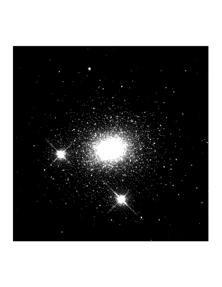
Figure 1: Mayall II $\equiv$ G1 as seen with the PC chip of the WFPC2 camera onboard the Hubble Space Telescope. The cluster is surrounded by two bright foreground stars. This image is a composite from F555W ($V$) and F814W ($I$) frames with a total exposure time of 2,200 seconds in $V$ and of 1,800 seconds in $I$. The field is 31.5″  $\times$  31.5″. North is 131^∘ clockwise from vertical direction and East is 41^∘ clockwise from vertical direction. (A non-degraded color version of this figure is available from the first author).

The globular cluster G1 belongs to our companion galaxy, Andromeda $\equiv$ M31. Resolved with difficulty from the ground (Djorgovski 1988, Heasley et al. 1988, Bendinelli et al. 1990), this huge swarm of stars appears as a bright flattened star cluster when observed with the Wide Field and Planetary camera WFPC2 onboard the Hubble Space Telescope (HST) (see Fig. 1). The integrated visual magnitude of this cluster, $V$ = 13.48 mag, corresponds to an absolute visual magnitude M_V = –10.94 mag, with $E(B-V)$ = 0.06 and a distance modulus $(m-M)_{M31}$ = 24.43 mag, implying a total luminosity of about $L_{V}$ $\sim$ 2 $\times$ $10^{6}L_{\odot}$ (Rich et al. 1996, Djorgovski et al. 1997).

The coordinates of G1, when compared to the coordinates of the center of M31 (see Table 1), place it at a projected distance of about 3^∘, i.e. 40 kpc, from the center of M31. This rather large projected distance is comparable to the distance between our Galaxy and the Large Magellanic Cloud. Nevertheless, both color-magnitude diagrams and radial velocities of G1 ($V_{r}{\rm(G1)}=-331\pm\ 24~{}{\rm km\thinspace s}^{-1}$) and M31 ($V_{r}{\rm(M31)}=-300\pm\ 4~{}{\rm km\thinspace s}^{-1}$ from 21cm HI line and $V_{r}{\rm(M31)}=-295\pm\ 7~{}{\rm km\thinspace s}^{-1}$ from optical lines), completely support the idea that this cluster belongs to the globular cluster system of M31. The values of the most important general parameters describing G1 are displayed in Table 1.

3 Observations

We use our observations obtained with the Planetary Camera (PC) of the HST/WFPC2, in the framework of a programme (PI Pascale Jablonka, ID = 5907) aiming at studying star clusters and stellar populations in M31 (see Jablonka et al. 1999, Jablonka et al. 2000). The PC pixel scale is 0.045^′′pix^-1. The four images of G1, taken with each of the F555W ($V$) and F814W ($I$) filters, have total integration times equal to 500 + 500 + 600 + 600 = 2,200 seconds in $V$ and to 400 + 400 + 500 + 500 = 1,800 seconds in $I$. Because of possible non-linearity in the bright concentrated core of G1, our rather deep exposures are supplemented with some shorter exposures from another programme (PI R. Michael Rich, ID = 5464). See Rich et al. (1996).

Fig. 1 displays an area of 31.5^′′ $\times$ 31.5^′′ from the original PC frames centered on the cluster. This image is a composite of all our $V$ and $I$ frames and provides a genuine indication of the relative colors of the stars. Although completely resolved, the cluster appears extremely compact, with a very steep surface brightness profile and an extremely bright and crowded core.

We determine the photometry using one of the presently best available algorithms for performing stellar photometry in crowded fields, viz., the ALLFRAME procedure developed by P. Stetson (1994). ALLFRAME is run on 700 $\times$ 700-pixel (31.5″ $\times$ 31.5″) sub-areas of the original (36″ $\times$ 36″) PC frames, avoiding the egdes of the frame and masking the two areas disturbed by the two bright foreground stars (Fig. 1). As ALLFRAME is now widely known and since our use of it is already described in Jablonka et al. (1999), here we mainly focus on the results. Given the very large projected distance between G1 and the core of M31 (40 kpc), it is worth mentioning that the number of M31 field stars in our PC field is negligible when compared to the number of G1 stars.

4 The Color-Magnitude Diagram of Mayall II $\equiv$ G1

Fig. 2 displays the two color-magnitude diagrams (CMDs) of G1, each of them containing the same 4903 stars. The left panel shows the $V$ vs. $V-I$ CMD, while the right panel displays the $I$ vs. $V-I$ CMD. The brightest stars at $V$$\sim$22.5 have color errors of $\sim$0.03, and stars at the level of the HB have color errors of $\sim$0.15 mag.

A first CMD of G1, reaching stars below the horizontal branch (HB), was published by Rich et al. (1996) based on HST Cycle 4 data, with total exposure times of 1,600 seconds in F555W and 1,200 seconds in F814W. Our exposure times are about 40% larger in $V$ and 50% larger in $I$. It is why, with the use of different methods/softwares in the photometric analysis, we can reach stars 0.5 mag and 1 mag fainter in $V$ and $I$, respectively.

These two CMDs show a relatively shallow RGB and a horizontal branch (HB) populated predominantly redward of the RR Lyrae instability strip. Both of these features suggest that G1 is a rather metal-rich stellar system. However, the CMD also reveals a blueward extension to the red HB clump composed of a small number of stars. All three of these populations were also noted by Rich et al.  (1996) in their CMD of G1. In particular, Rich et al.  (1996) pointed out that the blue extension to the HB could possibly be the result of a chemical abundance spread in G1. Indeed, the RGB does display a potentially significant color width. The statistical significance of this width is addressed below.

We note that the morphology of G1 HB is more reminiscent of the HB morphology observed in the dwarf spheroidal galaxy Andromeda I (Da Costa et al. 1996) than in the globular cluster 47 Tucanae  (Vazdekis et al. 2001). This fits some of the conclusions of this work, which unveiled some characteristics of the stellar population of G1, more typical of dwarf galaxies than of our classical view of globular clusters.

In order to measure the magnitude of the HB, we construct a luminosity function of the data and fit a Gaussian curve to the most prominent peak in this luminosity function. This procedure yields $V(HB)=25.34~{}\pm~{}0.07$. The quoted error is the result of adding, in quadrature, estimated errors of $\pm$ 0.05 in the determination of $V(HB)$ and $\pm$ 0.05 in the photometric zeropoint. This is in excellent agreement with the work of Rich et al. (1996) who obtained $V(HB)=25.32~{}\pm~{}0.05$. To estimate the metallicity of G1 in a way that is independent of the photometric zeropoint and the reddening, we rely upon the slope of the RGB as calibrated by Sarajedini et al. (2000). Utilizing their measurement technique and calibration leads to a value of [Fe/H] = $-0.95~{}\pm~{}0.09$ for the mean metal abundance of G1 on the scale of Zinn & West (1984). This abundance lies between the results of Rich et al. (1996) who obtained [Fe/H] $\sim$ –0.7 on the scale of Zinn & West (1984), a value close to that of 47 Tucanae, and those of Bonoli et al. (1987) and Brodie & Huchra (1990) who obtained [Fe/H] $\sim$ –1.2. In addition, our abundance is in accord with the estimate of Stephens et al. (2001) based on the $V-K(RGB)$ of G1; they find [Fe/H] = $-0.9~{}\pm~{}0.2$. Lastly, we can utilize the mean RGB color along with the calculated metal abundance and Equ. 1 of Sarajedini (1994) to compute the reddening of G1; we find $E(V-I)=0.05~{}\pm~{}0.02$.

Let us return now to the RGB color width apparent in the CMD of G1 (see Fig. 2). If this feature is significant, i.e. not caused entirely by the photometric errors, then we can argue strongly that there is a metallicity dispersion in G1. One method used to test this is to conduct artificial star experiments in order to estimate the true measurement error. To begin with, we select stars located along an RGB fiducial sequence. For each of two trials, we select 210 stars along this fiducial sequence and place them on the original PC1 frames under the constraint that no two artificial stars be within two PSF radii of each other. The resultant images are then reduced with the same procedure as the original PC images.

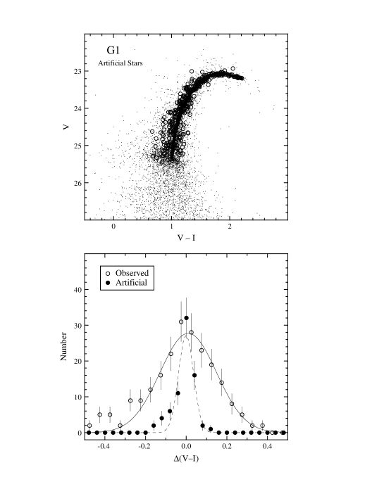
Figure 3: Artificial star experiments.  Upper panel: color-magnitude diagram where filled circles represent the original magnitudes and colors of the 420 artificial stars while the open circles are their recovered values. The dots represent the genuine G1 stars. Lower panel: the color widths of artificial and observed stars. The open circles show the color histogram of stars located 1.8 $\pm$ 0.25 magnitudes above the horizontal branch of G1 while filled circles show the color histogram of the artificial stars.

The filled circles in Fig. 3 represent the original magnitudes and colors of the 420 artificial stars while the open circles are their recovered values. We are interested in the color width of the artificial stars and how this compares with the observed RGB color width. The open circles in the lower panel of Fig. 3 show the color histogram of stars located 1.8 $\pm$ 0.25 magnitudes above the HB of G1. This location is chosen because it minimizes the influence of asymptotic giant branch stars (Da Costa & Armandroff 1990; Geisler & Sarajedini 1999). The filled circles represent the color histogram of the artificial stars around the fiducial sequence. Gaussian fits to these distributions yield $\sigma_{obs}=0.144~{}\pm~{}0.010$ for the observed width and $\sigma_{err}=0.037~{}\pm~{}0.004$ for the width due to photometric errors. Subtracting these quantities in quadrature gives $\sigma_{int}=0.139~{}\pm~{}0.011$ for the intrinsic width of the RGB. We note in passing that these artificial star experiments do not provide a complete and total assessment of the photometric errors. Other sources of error, e.g., such as residual flat-field non-uniformities and residual dark current, are not included in our photometric error estimates.

If we assume then that the intrinsic photometric width we calculate is due entirely to a metallicity dispersion in G1, what is the corresponding range in [Fe/H] ? To estimate this quantity, we turn to the standard RGB sequences of Da Costa & Armandroff (1990), which we use to construct a relation between [Fe/H] and $(V-I)_{0}$ at 1.8 mags above the HB of the six standard clusters in that study. The resultant relation is quadratic, which means that the [Fe/H] range it implies for G1 depends on the reddening we assume. The relation is:

$${\rm[Fe/H]}=-18.648+23.846(V-I)_{0}-7.906(V-I)_{0}^{2}$$

with $(V-I)_{0}$ = 1.39 at $V(HB)-1.8$. For example, if $E(V-I)$ = 0.10, then we infer a 1-$\sigma$ [Fe/H] dispersion of $\sigma_{{\rm[Fe/H]}}=~{}\pm~{}0.50$ dex; whereas if $E(V-I)$ = 0.05, then $\sigma_{{\rm[Fe/H]}}=~{}\pm~{}0.39$ dex. In any case, the metallicity dispersion in G1 is genuine and significant. In contrast, we applied the above technique to HST/WFPC2 photometry of the M31 globular cluster G219 (Neill 2001). These images were reduced in the same manner as those of G1 presented herein. We find that the color width of its RGB is fully consistent with the photometric errors as expected for a system with a negligible metallicity dispersion.

The fact that in their HST/NICMOS study of G1, Stephens et al. (2001) do not observe any spread in metallicity does neither contradict nor infirm our present result. This for two reasons. First, for any spread in [Fe/H], the corresponding spread in color is twice as small in the infrared $(J-K)$ than in the visible $(V-I)$. Second, their very small sample (they have about 200 stars while we have about 5,000 stars) would certainly affect statistically their measurement of any spread in metallicity.

The only other globular cluster known to exhibit a significant metal abundance range is $\omega$ Centauri, the giant Galactic globular cluster (see Jurcsik 1998 for a compilation of abundance measurements). Its range in [Fe/H] is roughly one dex (Norris & Da Costa 1995), which is quite similar to the range inferred by our estimates for G1.

5 Ellipticity, Position Angle, and Surface Brightness Profile

Surface photometry of the cluster is obtained from all available WFPC2 images, using the techniques described by Djorgovski (1988). We then combine the profiles extracted from different images, using the shorter, unsaturated exposures for the central part of the profile, and longer, higher S/N exposures (in which the cluster core was saturated) for the outer parts of the profiles.

Table 2 gives the ellipticity $\epsilon$ = $1-b/a$ and the position angle $PA$ as a function of the semi-major axis $a$, using the stack of all our F555W ($V$) frames along with short exposures obtained in the same filter and available in the STScI/HST archives. These data are displayed in Fig. 4. The ellipticity varies significantly with the semi-major axis $a$, from values smaller than $\epsilon$ = 0.1 in the innermost and outermost parts of the cluster, but with values larger than $\epsilon$ = 0.2 between 0.7^′′ and 7^′′, reaching a maximum of $\epsilon$ = 0.3 at $a$ = 2.1^′′. The mean ellipticity of G1 is $\epsilon$ $\simeq$ 0.2. The position angle $PA$ is not significantly variable for semi-major axis values $a$ larger than 0.2^′′. There is no significant evidence for twist of isophotes.

Table 3 gives the surface brightness $\mu_{V}$ and integrated $V$ magnitude as a function of the radius. The 72 points of this observed surface brightness profile are displayed in Fig. 5. There is no observational evidence of the presence of unbound stars and/or tidal tails surrounding G1, simply by the mere fact that we would need to reach stars a few magnitudes fainter than the turnoff to have a statistically significant sample of such escaping stars.

In order to convert the observed count rates to the $V$ band magnitudes, we used the standard transformations from Holtzman et al. (1995), assuming for the color of the cluster $(B-V)=0.84$ mag. Integration of the combined profile gives the total magnitude for the cluster, $V_{int}=13.48\pm 0.05$ mag, where the net estimated zero-point uncertainty includes both the errors due to the background subtraction, and the color transformation (they are of a comparable magnitude). This is in an excellent agreement with the values from van den Bergh (1969) and Reed et al. (1994), after applying the appropriate aperture and color corrections, which give 13.54 and 13.58 mag, respectively. We note that these ground-based measurements are likely to underestimate slightly the cluster brightness, due to the removal of the light covered by the bright foreground stars, which accounts for some of the systematic difference here. (None of these numbers include the Galactic extinction corrections.)

6 Mass Estimators

We have at our disposal two essential observational constraints allowing the mass determination of G1. First, our new determination of its surface brightness profile (see Table 3 and Fig. 5) from HST/WFPC2 images, providing essential structural parameters: the core radius $r_{c}$  = 0.14^′′ = 0.52 pc, the half-mass radius $r_{h}$  = 3.7^′′ = 14 pc, the tidal radius $r_{t}$  $\simeq$ 54^′′ = 200 pc, implying a concentration $c$ = log ($r_{t}/r_{c}$)  $\simeq$ 2.5. Second, our already published central velocity dispersion from KECK/HIRES spectra, providing an observed velocity dispersion $\sigma_{obs}$ = 25.1 km s^-1, and an aperture-corrected central velocity dispersion $\sigma_{p}$(0) = 27.8 km s^-1 (Djorgovski et al. 1997).

6.1 King model and Virial mass estimates

Masses of dynamical systems are difficult to evaluate, with different methods providing rather different results, and the scatter between the different values is generally much larger than their formal uncertainties. Consequently, it is worth presenting results from more than one method, thus giving a realistic estimate of the true uncertainty. We can first obtain simple mass estimates from King models and from the Virial theorem (see, e.g., Illingworth 1976).

The first estimate, the King mass $\mathcal{M}$_K, is given by the simple equation:

$${\mathcal{M}}_{K}~{}=~{}\rho_{c}r_{c}^{3}\mu~{}=~{}167~{}r_{c}\mu\sigma_{\circ}^{2}$$

where the core radius $r_{c}$ = 0.52 pc, the dimensionless quantity $\mu$ = 220 for $c$ = log ($r_{t}/r_{c}$)  = 2.5 (King 1966), and the central velocity dispersion $\sigma_{p}$(0) = 27.8 km s^-1. These values determine a total mass for the cluster of ${\mathcal{M}}_{tot}$ = 15 $\times$ ${{10^{6}\mathcal{M}_{\odot}}}$ with the corresponding ${\mathcal{M}}/L_{V}$ $\simeq$ 7.5 in solar units.

The second estimate, the Virial mass $\mathcal{M}$_Vir, is given by the simple equation:

$${\mathcal{M}}_{Vir}~{}=~{}670~{}r_{h}\sigma_{\circ}^{2}$$

where the half-mass radius $r_{h}$  = 14 pc and central velocity dispersion $\sigma_{p}$(0)  = 27.8 km s^-1. These values determine a total mass for the cluster of ${\mathcal{M}}_{tot}$ = 7.3 $\times$ ${{10^{6}\mathcal{M}_{\odot}}}$ with the corresponding ${\mathcal{M}}/L_{V}$ $\simeq$ 3.6 in solar units. The internal error of each of these mass estimates amounts to about 10%.

The large difference between these two estimates is not particular to the present cluster, but due to the idiosyncrasies of each method and typical of these two mass estimators applied to any globular cluster. See, e.g., Table 6 showing the results of similar mass estimates in the case of $\omega$ Centauri, the brightest and most massive Galactic globular cluster.

7 King-Michie model mass estimates

The two above observational constraints, viz., surface brightness profile and central velocity dispersion, allow the use of a multi-mass King-Michie model as defined by Gunn & Griffin (1979). See Meylan (1987) and Meylan et al. (1994, 1995) for the case of $\omega$ Centauri.

7.1 The model

The “lowered Maxwellian” energy dependence $[\exp(-A_{i}E)-1]$ has been shown (King 1966) to be a good approximation to the solution of the Fokker-Planck equation describing the phase-space diffusion and evaporation of stellar systems like globular clusters. Following Eddington (1916), Michie (1963) introduced possible radial ($\overline{v_{r}^{2}}$ $\not=$ $\overline{v_{\theta}^{2}}$ = $\overline{v_{\phi}^{2}}$)) anisotropy by a factor of the form $\exp(-\beta J^{2})$, where $J$ is the total angular momentum. Da Costa & Freeman (1976) showed that single-mass, isotropic King models are unable to fit the entire surface brightness profile of most globular clusters; they generalized these simple models to produce more realistic multi-mass models with full equipartition of energy in the centre.

In the present work, we use a multimass anisotropic King-Michie dynamical model, based on an assumed form for the phase-space distribution function in an approach similar to that of Gunn & Griffin (1979). Each of the twelve subpopulations used has an energy-angular momentum distribution function $f_{i}(E,J)$ such that:

$$f_{i}(E,J)\propto[\exp(-A_{i}E)-1]\exp(-\beta J^{2}).$$

Thermal equilibrium is assumed in the cluster center, because of the short expected relaxation time, in order to force $A_{i}$ to be proportional to the mean mass $\overline{m}_{i}$ of the stars in the subpopulation considered. A model is specified by an initial mass function (IMF) exponent $x$ (see below) and by four parameters: (i) the core radius $r_{c}$, (ii) the scale velocity $v_{s}$, (iii) the central value of the gravitational potential $W_{\circ}$, and (iv) the anisotropy radius $r_{a}$, beyond which the velocity dispersion tensor becomes increasingly radial.

7.2 The initial mass function

There is no observational determination of the present-day mass function in G1. Consequently, and in order to mimic a real cluster, main sequence (MS) stars, white dwarfs (wd) and heavier remnants (hr), such as neutron stars, are distributed into twelve different mass classes, adopting the usual power-law form for the initial mass function:

$$dN\propto m^{-{x}}d\thinspace\rm{log}(m)$$

where the exponent $x$ would equal 1.35 in the case of Salpeter (1955).

This initial mass function must be cut off at both extremities. The upper limit has neither dynamical nor photometric influence because of the rather small initial number of massive stars which have in any case already evolved into dark stellar remnants. This upper cutoff is chosen rather arbitrarily at 100 $M_{\odot}$. The lower limit is much more controversial because of the potential dynamical importance of numerous low-mass stars with low-luminosity. As found by Gunn & Griffin (1979), this lower mass cutoff, if it is low enough, does not significantly affect the cluster structure as traced by the giant stars. Numerous light stars do not change the quality of the fit, they simply increase the cluster mass and mass-luminosity ratio. The individual mass of the lightest stars is taken equal to 0.13 $M_{\odot}$.

Owing to the total lack of observational constraints on the present-day mass function along the main sequence, the exponent $x$ of the initial mass function is allowed to take different values in the following three mass intervals: $x_{hr}$, describing the heavy stellar remnants, resulting from the already evolved stars with initial masses in the mass range between 0.88 and 100 $M_{\odot}$; $x_{MS}^{up}$, describing the stars still on the main sequence, with initial masses in the mass range between 0.32 and 0.88 $M_{\odot}$; and $x_{MS}^{low}$ describing the stars still on the main sequence, with initial masses in the mass range between 0.13 and 0.32$M_{\odot}$.

7.3 The fit

Both the HST/WFPC2 images providing the surface brightness profile (Table 3 and Fig. 5), and the integrated light KECK/HIRES spectra providing the central velocity dispersion (Djorgovski et al. 1997) are heavily dominated by the light emitted by the brightest stars in G1. All of these stars, viz., the giants and subgiants visible in the CMD (see Fig. 2), have individual masses equal to or slightly smaller than the turnoff mass, and belong to the same subpopulation containing stars with individual masses in the range 0.63 to 0.88 $M_{\odot}$. Consequently, the fits between the models and the observations are made by using only this subpopulation, which contains the brightest members in the cluster, i.e., the giants, subgiants, turnoff stars, and the stars at the top of the main sequence. An acceptable model must match, simultaneously, first, the observed surface brightness profile, fitted by least squares to the integrated density profile of the subpopulation containing the bright stars, as determined by the model (see Fig. 5), and, second, the observed value of the velocity dispersion in the core of the cluster, which is unfortunately less constraining than the full velocity dispersion profile, as available, e.g., in the case of $\omega$ Centauri (Meylan et al. 1995). In addition to the above two requirements, a model has to recover the total luminosity of the cluster, viz., $M_{V}$ = –10.86 mag, to within 0.1 mag in order to be considered as satisfying.

7.4 Relaxation time

Two different “average” relaxation times are obtained for each model: a half-mass relaxation time and a central relaxation time. The term “average” means that these times depend on the mean stellar mass of the system, instead of being related to one particular species. Spitzer & Hart’s (1971) standard formula transforms into:

$$t_{rh}=(8.92~{}10^{5}yr)\times{{({\mathcal{M}}/{1m}{{}_{\odot}})^{1\over 2}}\over{({\overline{\mathcal{M}}}/{1m{{}_{\odot}}})}}\times{{({r_{h}/1pc})^{3\over 2}}\over{\rm{log}}({0.4{\mathcal{M}}}/{\overline{m}})}$$

where $\overline{m}$ is the mean stellar mass of all the stars in the cluster, ${\mathcal{M}}$ the total mass of the cluster, and $r_{h}$ the half-mass radius. From Lightman & Shapiro (1978), the central relaxation time is given by:

$$t_{r,\circ}=(1.55~{}10^{7}yr)\times{{(1{m}_{\odot}/\overline{{m}}_{\circ})}\over{\rm{log}}(0.5{\mathcal{M}}/\overline{m})}\times{{v_{s}}\over{1km/s}}\times({{r_{c}}\over{1pc}})^{2}$$

where $\overline{m}_{\circ}$ is the mean mass of all the particles in thermal equilibrium in the central parts, $v_{s}$ the velocity scale, and $r_{c}$ the core radius.

7.5 Results from King-Michie models

An extensive grid of about 150,000 models is computed in order to explore the parameter space defined by the Initial Mass Function (IMF) exponents $x$ (defined over three different mass ranges $x_{hr}$, $x_{MS}^{up}$, and $x_{MS}^{low}$, and where $x$ would equal 1.35 in the case of Salpeter 1955), the central gravitational potential $W_{\circ}$, and the anisotropy radius $r_{a}$.

Good models are considered as such not only on the basis of the $\chi^{2}$ of the surface brightness fit — the topology of the $\chi^{2}$ surface has no unique minimum — but also on the basis of their predictions of the integrated luminosity and mass-to-light of the cluster. We present hereafter results for the twelve models with lowest chi-square and fulfilling the other two requirements.

The different columns in Table 4 give, for each model defined by its index, the central value of the gravitational potential $W_{\circ}$; its MS mass function exponents $x_{MS}^{up}$ and $x_{MS}^{low}$; the fraction ${\mathcal{M}}_{tot}^{hr}$  of its total mass in the form of stellar remnants such as neutron stars and white dwarfs; its concentration $c$ = log ($r_{t}/r_{c}$), core radius $r_{c}$, half-mass radius $r_{h}$, and tidal radius $r_{t}$; its central value of the mass density $\rho_{c}$, mean mass density $\rho_{h}$ inside the half-mass radius, and mean mass density $\rho_{t}$ inside the tidal radius.

The different columns in Table 5 give, for each model defined by its index, the total mass ${\mathcal{M}}_{tot}$ of the cluster, in millions of solar masses, and its corresponding mass-to-light ratio ${\mathcal{M}}/L_{V}$, also in solar units; the half-mass relaxation time t_rh from Eq. (6), and central relaxation time t_r,∘ from Eq. (7).

Since the velocity dispersion profile is reduced to one single value — the central velocity dispersion — the models are not constrained as strongly as in the case of $\omega$ Centauri (Meylan et al. 1995), and equally good fits are obtained for rather different sets of parameters. Consequently, reliable results only relate to general parameters like the concentration and the total mass, but probably fail in any more detailed parameters. Nevertheless, very large areas of the parameter space can be eliminated with confidence since they never generate any successful models.

The IMF exponent $x_{hr}$, describing the amount of heavy stellar remnants, appears in all good models to be very close to $x$ = 1.35 (Salpeter 1955). The IMF exponent $x_{MS}^{up}$, describing the upper part of the MS, appears in all good models to be very close to $x$ = 1.55. The IMF exponent $x_{MS}^{low}$, describing the lower part of the MS, is not very well constrained; this is in agreement with Gunn & Griffin’s (1979) findings that the lower-mass stars do not significantly affect the cluster structure as traced by the giant stars. The fraction of the total mass of the cluster in the form of heavy stellar remnants (neutron stars and white dwarfs) is always in the range of 18 to 20%.

With a concentration $c$ = log ($r_{t}/r_{c}$) somewhere around 2.5, G1 is definitely a very concentrated globular cluster: all good models present clearly all the characteristics of a collapsed cluster. With its small core radius, G1 is hardly resolved in its central parts while its envelope exhibits an extended profile typical of a collapsed cluster (see also Djorgovski 1988). The core radius has a mean value of about $r_{c}$ $\simeq$ 0.52 pc, the half-mass radius $r_{h}$ $\simeq$ 13.5 pc, and the tidal radius, the most uncertain of these three radii, has a mean value of about $r_{t}$ $\simeq$ 200 pc. The corresponding mass densities have mean values of about $\rho_{c}$ = 4.7 $\times$ 10⁵ $M_{\odot}$pc^-3, $\rho_{h}$ = 7.5 $\times$ 10² $M_{\odot}$pc^-3, $\rho_{t}$ = 4.2 $\times$ 10^-1 $M_{\odot}$pc^-3.

With a total mass somewhere between 14 and 17 ${{10^{6}\mathcal{M}_{\odot}}}$, and with the corresponding mass-to-light ratio ${\mathcal{M}}/L_{V}$  between 6.9 and 8.1, G1 is significantly more massive than $\omega$ Centauri, maybe by up to a factor of three. These King-Michie mass estimates are in full agreement with the King mass estimate ($\mathcal{M}$_K = 15 $\times$ ${{10^{6}\mathcal{M}_{\odot}}}$  with ${\mathcal{M}}/L_{V}$ $\simeq$ 7.5), while the Virial mass estimate ($\mathcal{M}$_Vir = 7.3 $\times$ ${{10^{6}\mathcal{M}_{\odot}}}$ with ${\mathcal{M}}/L_{V}$ $\simeq$ 3.6) is smaller by about a factor of two. It is worth mentioning that such a difference between King and Virial mass estimates is not specific to G1: the same factor of about two is also observed between the King-Michie and Virial mass estimates of any cluster. See, e.g., in Table 6 the comparison of the results obtained for G1 and $\omega$ Centauri (Meylan & Mayor 1986, Meylan 1987, Meylan et al. 1995, and this paper).

8 Is Mayall II $\equiv$ G1 a genuine globular cluster ?

We reach the following conclusions: (i) G1 is only the second globular cluster in which we observe a significant metallicity spread among its giant stars, $\omega$ Centauri being the first such case; (ii) All mass estimates (Table 6) give a total mass for G1 equal to as much as three times the total mass of $\omega$ Centauri; (iii) With $c$ = log ($r_{t}/r_{c}$) $\simeq$ 2.5, G1 is significantly more concentrated than 47 Tucanae, which is a massive Galactic globular cluster considered on the verge of core collapse; all G1 structural parameters deduced from its surface brightness profile as well as the model densities are typical of a collapsed cluster; (iv) G1 is the heaviest of the weighed globular clusters.

Although $\omega$ Centauri is by far the brightest and most massive globular cluster in our Galaxy, G1 may not be the only such massive globular cluster belonging to M31. This galaxy, which has about three times as many globular clusters as our Galaxy, has at least three other bright clusters which have central velocity dispersions larger than 20 km s^-1 (Djorgovski et al. 1997). Unfortunately, so far, G1 is the only such cluster imaged with the high spatial resolution of the HST/WFPC2 camera, and consequently the only such massive cluster with a high quality surface brightness profile and known structural parameters. G1 and the other three bright M31 globular clusters represent probably the high-mass and high-luminosity tails of the mass and luminosity distributions of the rich population of M31 globular clusters.

The above large mass estimates, implying a rather deep potential well, obviously relate to the metallicity spread whose origin is still unknown. There are essentially three different scenarios to explain such a metallicity spread: (i) metallicity self-enrichment in the globular cluster, (ii) primordial metallicity inhomogeneity in the proto-cluster cloud, and (iii) the present globular cluster is merely the remaining core of a previously larger entity.

Even more so than $\omega$ Centauri, G1 could be a kind of transition step between globular clusters and dwarf elliptical galaxies, in being the remaining core of a dwarf galaxy whose envelope would have been severely pruned by tidal shocking due to the bulge and disk of its host galaxy, M31.

Kormendy (1985, 1987, 1994) used the four following quantities — the central surface brightness $\mu$(0,$V$), the central velocity dispersion $\sigma_{p}$(0), the core radius $r_{c}$, and the total absolute magnitude M_V — in order to define various planes from combinations of two of the above four parameters, e.g., ($\mu$(0,$V$) vs. log $r_{c}$). In all four planes plotted by Kormendy (1985, his Fig. 3), the various stellar systems segregate into three well separated sequences: (i) ellipticals and bulges, (ii) dwarf ellipticals, and (iii) globular clusters. When plotted on any of the four planes, G1 appears always on the sequence of globular clusters, and cannot be confused or assimilated with either ellipticals and bulges or dwarf ellipticals. The same is true for $\omega$ Centauri. Consequently, in spite of their large masses and internal stellar metallicity spreads, G1 and $\omega$ Centauri look like genuine bright and massive globular clusters. But where on these diagrams would the remaining cores of dwarf galaxies be located ?

Because of its very large central velocity dispersion, M32 could not be the progenitor of a star cluster like G1 (van der Marel et al. 1998). But this is not true for the nucleated dwarf galaxy NGC 205, which has a central velocity dispersion similar to G1 (Carter & Sadler 1990, Held et al. 1990, Bender et al. 1991). The nucleus of NGC 205 is the only one for which the values of the four parameters used in Kormendy’s diagrams are known, viz., the central velocity dispersion $\sigma_{p}$(0)  = 30 km s^-1  (Bender et al.  1991), the central surface brightness $\mu$(0,$V$) = 12.84 mag arcsec^-2, the core radius $r_{c}$ = 0.35 pc, and the total absolute magnitude M_V = –9.6 (Jones et al. 1996). These values place NGC 205 nucleus, in the Kormendy’s diagrams, very close to G1, right on the sequence of the globular clusters. Although this does not prove that all (massive) globular clusters are the remnant cores of nucleated dwarf galaxies, it shows that at least the nucleus of one such dwarf exhibits characteristics identical to those of globular clusters. It would be useful to know more about the nuclei of other dwarf galaxies.

Of these massive globular clusters, the most nearby, $\omega$ Centauri, is naturally the best studied, nevertheless without decreasing the number of its conundrums. For instance, recent photometric (Anderson 1997) and kinematic (Norris et al. 1997) studies show that $\omega$ Centauri presents numerous characteristics about its stellar populations which remain without any explanation, if not completely puzzling. Presently, only the anti-correlation of metallicity with age (Hughes & Wallerstein 2000) and the unusual patterns of CN elements (Hilker & Richtler 2000) recently observed in $\omega$ Centauri suggest¡ that this cluster enriched itself over a timescale of about 3 Gyr. This contradicts the general idea that all the stars in a globular cluster are coeval, and may favor the origin of $\omega$ Centauri  as being the remaining core of a larger entity, e.g., of a former nucleated dwarf elliptical galaxy. Such a general idea had already been suggested by Zinnecker (1988) and Freeman (1993). In any case, the very massive globular clusters, by the mere fact that their large masses imply complicated stellar and dynamical evolution, may blur the former clear (or simplistic) difference between globular clusters and dwarf galaxies.

Table 1: General information about Mayall II $\equiv$ G1

Parameters	Mayall II $\equiv$ G1
$\alpha$ G1 (J2000)	00h 32m 46.6s
$\delta$ G1 (J2000)	+39o 34′ 40′′
$\alpha$ M31 (J2000)	00h 42m 44.5s
$\delta$ M31 (J2000)	+41o 16′ 29′′
Distance $D$ to M31	770 kpc
Color excess $E(B-V)$	0.06 mag
True distance modulus $(m-M)$	24.42 mag
Observed magnitude $V$	13.48 mag
Absolute magnitude $M_{V}$	–10.94 mag
Central $V$ surf bright $\mu$(0,$V$)	13.47 mag arcsec-2
Age	$\sim$ 15 Gyr
Metallicity [Fe/H]	–0.95
Mean ellipticity $\epsilon$	0.2
Radial velocity $V_{r}$	–331 $\pm$ 24 km s-1
Velocity dispersion $\sigma_{obs}$	25.1 km s-1
Vel. dis. aperture corrected $\sigma$(0)	27.8 km s-1

Table 2: Mayall II $\equiv$ G1: ellipticity $\epsilon$ and position angle $PA$ as a function of the semi-major axis $a$

$a$	$\epsilon$	$PA$
[arcsec]		[degree]
0.091	0.139 $\pm$ 0.010	109.2 $\pm$ 1.0
0.137	0.151 $\pm$ 0.010	109.2 $\pm$ 1.0
0.182	0.087 $\pm$ 0.010	105.3 $\pm$ 1.0
0.228	0.113 $\pm$ 0.010	110.0 $\pm$ 1.0
0.273	0.112 $\pm$ 0.010	114.4 $\pm$ 1.0
0.319	0.110 $\pm$ 0.010	120.6 $\pm$ 1.0
0.364	0.115 $\pm$ 0.010	122.5 $\pm$ 1.0
0.410	0.120 $\pm$ 0.010	123.7 $\pm$ 1.0
0.455	0.123 $\pm$ 0.010	124.0 $\pm$ 1.0
0.501	0.127 $\pm$ 0.010	123.3 $\pm$ 1.0
0.546	0.133 $\pm$ 0.010	123.5 $\pm$ 1.0
0.591	0.149 $\pm$ 0.010	123.6 $\pm$ 1.0
0.637	0.178 $\pm$ 0.010	123.5 $\pm$ 1.0
0.683	0.192 $\pm$ 0.010	123.4 $\pm$ 1.0
0.728	0.192 $\pm$ 0.010	123.4 $\pm$ 1.0
0.774	0.192 $\pm$ 0.010	123.5 $\pm$ 1.0
0.819	0.193 $\pm$ 0.010	122.4 $\pm$ 1.0
0.865	0.193 $\pm$ 0.010	120.5 $\pm$ 1.0
0.910	0.193 $\pm$ 0.010	119.8 $\pm$ 1.0
0.956	0.195 $\pm$ 0.010	119.8 $\pm$ 1.0
1.046	0.227 $\pm$ 0.029	119.1 $\pm$ 1.6
1.183	0.235 $\pm$ 0.011	119.1 $\pm$ 1.7
1.342	0.199 $\pm$ 0.024	117.4 $\pm$ 2.3
1.501	0.193 $\pm$ 0.015	116.2 $\pm$ 2.9
1.683	0.242 $\pm$ 0.030	120.5 $\pm$ 5.9
1.888	0.269 $\pm$ 0.017	126.1 $\pm$ 1.3
2.115	0.299 $\pm$ 0.020	124.4 $\pm$ 2.0
2.387	0.251 $\pm$ 0.031	122.8 $\pm$ 2.5
2.661	0.250 $\pm$ 0.029	124.0 $\pm$ 3.2
2.979	0.231 $\pm$ 0.018	123.5 $\pm$ 1.9
3.564	0.216 $\pm$ 0.021	122.0 $\pm$ 11.9
4.495	0.234 $\pm$ 0.023	123.0 $\pm$ 11.5
5.653	0.208 $\pm$ 0.032	121.0 $\pm$ 10.0
7.105	0.254 $\pm$ 0.062	120.6 $\pm$ 9.0
8.944	0.183 $\pm$ 0.026	123.5 $\pm$ 8.4
11.259	0.146 $\pm$ 0.085	129.3 $\pm$ 6.1

Table 3: Mayall II $\equiv$ G1: surface brightness $\mu_{V}$ and integrated $V$ magnitude as a function of the radius

$R$	$\mu_{V}$	$V_{int}$		$R$	$\mu_{V}$	$V_{int}$
[arcsec]	[mag]	[mag]		[arcsec]	[mag]	[mag]
0.039	13.467 $\pm$ 0.019	19.268		1.243	17.307 $\pm$ 0.055	14.206
0.061	13.557 $\pm$ 0.022	18.321		1.251	17.329 $\pm$ 0.055	14.202
0.066	13.574 $\pm$ 0.014	18.161		1.512	17.855 $\pm$ 0.094	14.096
0.074	13.610 $\pm$ 0.015	17.930		1.586	17.953 $\pm$ 0.099	14.073
0.085	13.657 $\pm$ 0.026	17.655		1.608	17.963 $\pm$ 0.095	14.066
0.089	13.689 $\pm$ 0.032	17.566		1.826	18.241 $\pm$ 0.091	14.005
0.100	13.745 $\pm$ 0.019	17.345		2.025	18.483 $\pm$ 0.085	13.958
0.108	13.747 $\pm$ 0.020	17.198		2.189	18.673 $\pm$ 0.083	13.925
0.130	13.877 $\pm$ 0.014	16.854		2.206	18.722 $\pm$ 0.087	13.922
0.138	13.896 $\pm$ 0.017	16.748		2.585	19.107 $\pm$ 0.094	13.861
0.157	14.026 $\pm$ 0.023	16.523		2.665	19.191 $\pm$ 0.099	13.850
0.176	14.093 $\pm$ 0.016	16.332		2.980	19.497 $\pm$ 0.097	13.812
0.186	14.144 $\pm$ 0.014	16.241		3.219	19.746 $\pm$ 0.094	13.788
0.189	14.163 $\pm$ 0.012	16.215		3.299	19.795 $\pm$ 0.099	13.781
0.225	14.329 $\pm$ 0.014	15.940		3.889	20.224 $\pm$ 0.114	13.734
0.228	14.357 $\pm$ 0.014	15.921		4.056	20.322 $\pm$ 0.116	13.723
0.253	14.472 $\pm$ 0.017	15.767		4.211	20.447 $\pm$ 0.114	13.714
0.276	14.574 $\pm$ 0.020	15.644		4.697	20.715 $\pm$ 0.119	13.687
0.287	14.634 $\pm$ 0.025	15.590		5.377	21.011 $\pm$ 0.117	13.656
0.333	14.857 $\pm$ 0.027	15.396		5.520	21.074 $\pm$ 0.117	13.650
0.344	14.882 $\pm$ 0.027	15.355		5.675	21.175 $\pm$ 0.117	13.644
0.367	14.988 $\pm$ 0.030	15.276		6.855	21.721 $\pm$ 0.141	13.605
0.403	15.129 $\pm$ 0.029	15.166		6.863	21.692 $\pm$ 0.135	13.605
0.468	15.354 $\pm$ 0.027	14.999		7.514	21.944 $\pm$ 0.148	13.589
0.469	15.354 $\pm$ 0.029	14.996		8.281	22.242 $\pm$ 0.175	13.572
0.486	15.423 $\pm$ 0.032	14.958		8.758	22.380 $\pm$ 0.187	13.563
0.588	15.786 $\pm$ 0.050	14.767		10.002	22.768 $\pm$ 0.226	13.543
0.598	15.808 $\pm$ 0.050	14.752		10.226	22.784 $\pm$ 0.225	13.540
0.638	15.926 $\pm$ 0.051	14.693		11.179	23.063 $\pm$ 0.266	13.528
0.710	16.133 $\pm$ 0.055	14.600		12.084	23.283 $\pm$ 0.320	13.518
0.763	16.287 $\pm$ 0.058	14.541		13.919	23.849 $\pm$ 0.458	13.502
0.858	16.580 $\pm$ 0.066	14.452		14.269	23.991 $\pm$ 0.516	13.500
0.868	16.577 $\pm$ 0.064	14.444		14.598	24.113 $\pm$ 0.556	13.498
0.974	16.836 $\pm$ 0.065	14.363		17.632	24.941 $\pm$ 0.987	13.484
1.036	16.940 $\pm$ 0.064	14.322		18.214	25.051 $\pm$ 1.054	13.482
1.182	17.188 $\pm$ 0.057	14.237		18.945	25.190 $\pm$ 1.137	13.480

Table 4: Mayal II $\equiv$ G1: multi-mass King-Michie model parameters

model	$W_{\circ}$	$x_{MS}^{up}$	$x_{MS}^{low}$	$M_{hr+wd}$	$c$	$r_{c}$	$r_{h}$	$r_{t}$	$\rho_{\circ}$	$\rho_{h}$	$\rho_{t}$
index				%	log ($r_{t}/r_{c}$)	[pc]	[pc]	[pc]	[$M_{\odot}$pc-3]	[$M_{\odot}$pc-3]	[$M_{\odot}$pc-3]
(1)	(2)	(3)	(4)	(5)	(6)	(7)	(8)	(9)	(10)	(11)	(12)
1	15.25	1.50	–0.50	20	2.49	0.53	12.3	163	4.7E+5	8.9E+2	7.8E–1
2	15.50	1.55	–0.50	20	2.59	0.52	13.2	199	4.9E+5	7.7E+2	4.5E–1
3	15.50	1.55	–0.40	19	2.57	0.52	13.2	193	4.8E+5	7.7E+2	4.9E–1
4	15.50	1.55	–0.30	19	2.55	0.53	13.2	187	4.7E+5	7.8E+2	5.4E–1
5	15.75	1.55	0.00	18	2.61	0.52	13.9	212	4.8E+5	6.9E+2	3.9E–1
6	15.50	1.60	–0.50	19	2.56	0.53	13.2	193	4.7E+5	7.7E+2	4.9E–1
7	15.50	1.60	–0.40	19	2.55	0.53	13.2	187	4.6E+5	7.7E+2	5.4E–1
8	15.75	1.60	–0.30	19	2.65	0.51	14.1	230	4.9E+5	6.7E+2	3.1E–1
9	15.75	1.60	–0.20	18	2.63	0.52	14.0	221	4.8E+5	6.8E+2	3.5E–1
10	15.75	1.60	–0.10	18	2.61	0.52	14.0	213	4.7E+5	6.8E+2	3.9E–1
11	15.75	1.60	0.00	18	2.59	0.53	14.0	205	4.6E+5	6.9E+2	4.4E–1
12	16.00	1.60	+0.20	17	2.68	0.52	15.0	245	4.8E+5	5.9E+2	2.6E–1

Table 5: Mayal II $\equiv$ G1: multi-mass King-Michie model parameters

model	${\mathcal{M}}_{tot}$	${\mathcal{M}}/L_{V}$	trh	tr,∘
index	[${{10^{6}\mathcal{M}_{\odot}}}$]	[$\odot$]	[${{10^{9}}}$yr]	[${{10^{6}}}$yr]
(1)	(2)	(3)	(4)	(5)
1	14	6.9	43	15
2	15	7.1	50	14
3	15	7.2	50	15
4	15	7.3	50	15
5	16	7.6	57	14
6	15	7.3	51	15
7	15	7.3	51	15
8	16	7.5	57	14
9	16	7.6	57	15
10	16	7.7	58	15
11	16	7.8	58	15
12	17	8.1	67	15

Table 6: Three different mass estimates for the two globular clusters Mayall II $\equiv$ G1 and NGC 5139 $\equiv$ $\omega$ Centauri

Mass	G1	G1	$\omega$ Cen	$\omega$ Cen
Estimator	mass [${{10^{6}\mathcal{M}_{\odot}}}$]	${\mathcal{M}}/L_{V}$[$\odot$]	mass [${{10^{6}\mathcal{M}_{\odot}}}$]	${\mathcal{M}}/L_{V}$[$\odot$]
King	15.	7.5	4.3	3.5
Virial	7.3	3.6	3.0	2.4
King-Michie	14-17	6.9-8.1	5.1	4.1

Figure 2: Color-magnitude diagram (CMD) of Mayall II $\equiv$ G1. The left panel shows the $V$ vs. $V-I$ CMD, while the right panel displays the $I$ vs. $V-I$ CMD. Each panel contains the same 4903 stars.

Figure 4: Ellipticity and position angle as a function of the semi-major axis, for Mayall II $\equiv$ G1, using the stack of all F555W ($V$) frames obtained with the PC chip of the WFPC2 camera onboard the Hubble Space Telescope.

Figure 5: Surface brightness profile of the globular cluster Mayall II $\equiv$ G1, from HST/WFPC2 shallow and deep images in F555W $\simeq$ $V$ filter; the continuous line represents a King-Michie model (first model in Table 4) fitted to the observed profile (Meylan et al. 1999).

References

- (1) Ajhar E.A., Grillmair C.J., Lauer T.R., et al., 1996, AJ, 111, 1110
- (2) Anderson J., 1997, Ph.D. thesis, University of California, Berkeley
- (3) Barmby P. Huchra J.P., Brodie J.P., Forbes D.A., Schroder L.L., Grillmair C.J., 2000, AJ, 119, 727
- (4) Battistini P., Bònoli F., Braccesi A., et al., 1987, A&AS,67, 447
- (5) Bender R., Paquet A., Nieto J.-L., 1991, A&A, 246, 349
- (6) Bendinelli O., Zavatti F., Parmeggiani G., Djorgovski, S.G., 1990, AJ, 99, 774
- (7) Bonoli F., Fusi Pecci F., Delpino F., Federici L., 1987, A&A, 185, 25
- (8) Brodie J.P., Huchra J.P., 1990, ApJ, 362, 503
- (9) Carter D., Sadler E.M., 1990, MNRAS, 245, 12P
- (10) Da Costa G. S., Armandroff T. E., 1990, AJ, 100, 162
- (11) Da Costa G.S., Freeman K.C., 1976, ApJ, 206, 128
- (12) Da Costa G.S., Armandroff T.E., Caldwell N., Seitzer P., 1996, AJ, 112, 2576
- (13) Djorgovski S.G., 1988, in IAU Symposium 126, Globular Cluster Systems in Galaxies, eds. J.E. Grindlay, A.G.D. Philip, (Dordrecht: Kluwer), pp. 333-346
- (14) Djorgovski S.G., Meylan G., 1994, AJ, 108, 1292
- (15) Djorgovski S.G., Gal R.R., McCarthy J.K., Cohen J.G., de Carvalho R.R., Meylan G., Bendinelli O., Parmeggiani G., 1997, ApJL, 474, L19
- (16) Eddington A.S., 1916, MNRAS, 76, 572
- (17) Freeman K.C., 1993, in Galactic Bulges, IAU symp. 153, p. 263
- (18) Fusi Pecci F., Battistini P., Bendinelli O., et al., 1994, A&A, 284, 349
- (19) Fusi-Pecci F., Buonanno R., Cacciari C., et al., 1996, AJ, 112, 1461
- (20) Geisler D., Sarajedini A., 1999, AJ, 117, 308
- (21) Grillmair C.J., Ajhar E.A., Faber S.M., et al., 1996, AJ, 111, 2293
- (22) Gunn J.E., Griffin R.F., 1979, AJ, 84, 752
- (23) Harris W.E., 1991, ARA&A, 29, 543
- (24) Heasley J. N., Friel E.D., Christian C.A., Janes K.A., 1988, AJ, 96, 1312
- (25) Held E.V., Mould J.R., de Zeeuw P.T., 1990, AJ, 100, 415
- (26) Hilker M., Richtler T., 2000, A&A, 362, 895
- (27) Holtzman, J., et al., 1995, PASP, 107, 156
- (28) Hughes J., Wallerstein G., 2000, AJ, 119, 1225
- (29) Illingworth G., Illingworth W., 1976, ApJS, 30, 227
- (30) Inman R.T., Carney B.W., 1987, AJ, 93, 1166
- (31) Jablonka P., Bridges T.J., Sarajedini A., Meylan G., Maeder A., Meynet G., 1999, ApJ, 518, 627
- (32) Jablonka P., Courbin F., Meylan G., Sarajedini A., Bridges T.J., Magain P., 2000, A&A, 359, 131
- (33) Jones D.H., Mould J.R., Watson A.M., et al., 1996, ApJ, 466, 742
- (34) Jurcsik J. 1998, ApJ, 506, L113
- (35) King I.R., 1966, AJ, 71, 64
- (36) Kormendy J., 1985, ApJ, 295, 73
- (37) Kormendy J., 1987, in Nearly Normal Galaxies: From the Planck Time to the Present, eds. S.M. Faber, (New York: Springer-Verlag), pp. 163-174.
- (38) Kormendy J., Bender R., 1994, in ESO/OHP workshop on Dward Galaxies, eds. G. Meylan, P. Prugniel (Garching: ESO), pp. 161-174
- (39) Lightman A.P., Shapiro S.L., 1978, Rev. Mod. Phys., 50, 437
- (40) Meylan G., 1987, A&A, 184, 144
- (41) Meylan G., 2000, in The Galactic Halo: from Globular Clusters to Field Stars, eds. A. Noels, et al., (Liège: Université de Liège), pp. 543-559
- (42) Meylan G., Heggie D.C., 1997, A&ARev, 8, 1
- (43) Meylan G., Jablonka P., Djorgovski S.G., Sarajedini A., Bridges T., Rich R.M., 1997, BAAS, 29, 1367
- (44) Meylan G., Mayor M., 1986, A&A, 166, 122
- (45) Meylan G., Mayor M., Duquennoy A., Dubath P., 1994, BAAS, 26, 956
- (46) Meylan G., Mayor M., Duquennoy A., Dubath P., 1995, A&A, 303, 761
- (47) Meylan G., Sarajedini A., Jablonka P., Djorgovski S.G., Bridges T., Rich R.M., 2000, BAAS, 32, 1440
- (48) Michie R.W., 1963, MNRAS, 126, 499
- (49) Neill J.D., 2001, priv. communication
- (50) Norris J.E., Da Costa G.S., 1995, ApJ, 441, L81
- (51) Norris J.E., Freeman K.C., Mayor M., Seitzer P., 1997, ApJ, 487, L187
- (52) Reed L.G., Harris G.L.H., Harris W.E., 1994, AJ, 107, 555
- (53) Rich R.M., Mighell K.J., Freedman W.L., Neill J.D., 1996, AJ, 111, 768
- (54) Salpeter E.E., 1955, ApJ, 121, 161
- (55) Sarajedini A., 1994, AJ, 107, 618
- (56) Sarajedini A., Geisler D., Schommer R., Harding P., 2000, AJ, 120, 2437
- (57) Spitzer L. Jr., Hart M.H., 1971, ApJ, 164, 399
- (58) Stephens A.W., Frogel J.A., Freedman W., Gallart C., Jablonka P., Ortolani S., Renzini A., Rich R. M., Davies R., 2001, in press (astro-ph/0011047)
- (59) Stetson P.B., 1994, PASP, 106, 250
- (60) van den Bergh, S. 1969, ApJS, 19, 145
- (61) van der Marel R.P., Cretton N., de Zeeuw P.T., Rix H.-W., 1998, ApJ, 493, 613
- (62) Vazdekis A., Salaris M., Arimoto N., Rose J.A., 2001, ApJ, 549, 274
- (63) Zinn R., West M.J., 1984, ApJS, 55, 45
- (64) Zinnecker H., Keable C.J., Dunlop J.S., Cannon R.D., Griffiths W.K., 1988, in IAU Symposium 126, Globular Cluster Systems in Galaxies, eds. J.E. Grindlay, A.G.D. Philip, (Dordrecht: Kluwer), pp. 603-701