Hydrodynamical Simulations of Jet- and Wind-driven Protostellar Outflows

Abstract

We present two-dimensional hydrodynamical simulations of both jet- and wind-driven models for protostellar outflows in order to make detailed comparisons to the kinematics of observed molecular outflows. The simulations are performed with the ZEUS-2D hydrodynamical code using a simplified equation of state, simplified cooling and no external heating, and no self-gravity.

In simulations of steady jets, swept-up ambient gas forms a thin shell that can be identified as a molecular outflow. We find a simple ballistic bow-shock model is able to reproduce the structure and transverse velocity of the shell. Position-velocity (PV) diagrams for the shell cut along the outflow axis show a convex spur structure with the highest velocity at the bow tip, and low-velocity red and blue components at any viewing angle. The power-law index of the mass-velocity relationship ranges from 1.5 to 3.5, depending strongly on the inclination. If the jet is time-variable, the PV diagrams show multiple convex spur structures and the power-law index becomes smaller than the steady jet simulation.

In simulations of isothermal steady wide-angle winds, swept-up ambient gas forms a thin shell which at early stages has a similar shape to the shell in the jet-driven model; it becomes broader at later times. We find the structure and kinematics of the shell is well described by a momentum-conserving model similar to that of Shu et al. (1991). In contrast to the results from jet simulations, the PV diagrams for the shell cut along the outflow axis show a lobe structure tilted with source inclination, with components that are primarily either red or blue unless the inclination is nearly in the plane of sky. The power-law index of the mass-velocity relationship ranges from 1.3 to 1.8. If the wind is time-variable, the PV diagrams also show multiple structures, and the power-law index becomes smaller than the steady wind simulation.

Comparing the different simulations with observations, we find that some outflows, e.g., HH 212, show features consistent with the jet-driven model, while others, e.g., VLA 05487, are consistent with the wind-driven model.

1 Introduction

Protostellar jets and molecular outflows are often associated with the same young stellar objects (Lada, 1985; Bachiller, 1996). They provide unique information about the mass-loss properties of young stars and give insight into the star forming process itself. However, the physics connecting the two phenomena remains unclear.

Protostellar jets are generally detected as optical jets in [SII] $\lambda\lambda$6716, 6731 and H$\alpha$ (Ray, et al., 1996; Reipurth et al., 1999), as infrared jets in H₂ (Coppin, Davis, & Micono, 1998; Zinnecker, McCaughrean, & Rayner, 1998), or as radio jets in the radio continuum (Anglada, 1995). They are also observed in some molecules, e.g., SiO (L 1448, Dutrey, Guilloteau & Bachiller, 1997) and CO (HH 211, Gueth & Guilloteau, 1999). Generally, the jets are highly collimated structures, consisting of a series of knots and bow-shocks, extending as far as a few pc out from the central stars (e.g., HH 111, Reipurth, Bally, & Devine, 1997).

Molecular outflows are generally seen in CO and some other molecules, as bipolar quasi-conical or -parabolic structures surrounding the jet. The observational properties of molecular outflows are summarized in Masson & Chernin (1993), Bachiller (1996), Cabrit, Raga & Gueth (1997), and Richer et al. (2000). Molecular outflows are much more massive and normally less well collimated than the jets. They have a simple power-law mass distribution with velocity (Masson & Chernin, 1992; Stahler, 1994). In many cases, the velocities in the molecular outflows increase with distance from the source. At low velocities, the outflow appears as a limb-brightened shell surrounding a cavity, while at high velocities the outflow sometimes becomes more jet-like. There is also evidence that outflow velocities are directed primarily along the major axis of the outflow, with little overlap of blueshifted and redshifted emission within the same flow lobe (Meyers-Rice & Lada, 1991; Lada & Fich, 1996). In a small sample of outflows known to be associated with jets, position-velocity (PV) diagrams constructed in a cut along the outflow axis reveal two different kinematic structures: a parabolic structure originating at the driving source, and a convex structure with the high velocity tip near the H₂ bow shock structure (Lee et al., 2000).

A number of models have been proposed to explain the connection between protostellar jets and molecular outflows. Currently, models in which the outflows are driven either by a highly collimated jet (Raga & Cabrit, 1993; Masson & Chernin, 1993; Chernin et al., 1994) or by a wider-angle wind (Shu et al., 1991; Li & Shu, 1996b; Shu et al., 2000) are the most popular. In the former, the bow shock originating at the head of the jet sweeps the ambient material into a thin shell which might be identified as the molecular outflow. A number of simulations have been carried out to investigate the hydrodynamics of protostellar jets (Blondin, Konigl & Fryxell, 1989; Blondin, Fryxell & Konigl, 1990; Stone & Norman, 1993a, b, 1994; Biro & Raga, 1994; Suttner et al., 1997; Smith, Suttner, & Yorke, 1997; Downes & Ray, 1999). Such simulations show that steady, collimated jets are able to produce qualitatively the structure and kinematics of some molecular outflows, e.g., NGC 2264G (Smith, Suttner, & Yorke, 1997). In the wind-driven shell model, ambient material is swept up by a radial wide-angle magnetized wind. If the wind has an axial density gradient, the core of the wind can take on the appearance of a collimated jet (Shu et al., 1995; Ostriker, 1997; Shang et al., 1998). If thermal pressure is unimportant, the molecular outflow is momentum-driven (Shu et al., 1991; Masson & Chernin, 1992; Li & Shu, 1996b; Matzner & McKee, 1999); the resulting structure and kinematics are found to be able to describe e.g., HH 111 CO outflow (Nagar et al., 1997). If there is little or no cooling of the shocked wind and ambient gas, the dynamics of the outflow can be different from the momentum-driven shell model (Frank & Mellema, 1996; Delamarter, Frank & Hartmann, 2000).

In this paper, we present comparisons of two-dimensional hydrodynamical simulations of both jet- and wind-driven outflow models with observed molecular outflows in order to test which aspects of each model provides a good fit to the observed kinematics. We also present the first quantitative comparison of the structure and kinematics of the swept-up shells found in the simulations (which is identified as a molecular outflow) to new and existing analytical models of jet-driven bow shocks and wide-angle winds, respectively. Since we concentrate on the dynamics of the large-scale shell, our simulations are performed with the ZEUS-2D hydrodynamical code using approximate cooling rates, and moderate numerical resolution. We calculate the PV diagrams as well as mass-velocity relationships for the shells and compare them with high-resolution CO observations of a number of molecular outflows. Calculations are presented for both steady and time-variable (pulsed) jets and winds. Our primary goal is to use the simulations to provide a survey of the dynamics of outflows for a wide variety of models (winds versus jets, pulsed versus steady), in order to test which models best fit the observations.

2 Equations and Numerical Method

The two-dimensional hydrodynamic code, ZEUS 2D (developed by Stone & Norman, 1992), is used to solve the equations of hydrodynamics,

$$\frac{\partial{\rho}}{\partial{t}}+\nabla\cdot(\rho{\bf v})=0$$ (1)

$$\frac{\partial{\rho{\bf v}}}{\partial{t}}+\nabla\cdot(\rho{\bf v}{\bf v})=-\nabla p+\rho\nabla\Phi$$ (2)

$$\frac{\partial{e}}{\partial{t}}+\nabla\cdot(e{\bf v})=-p\nabla\cdot{\bf v}-n^{2}\Lambda$$ (3)

where $\rho$, ${\bf v}$, $p$, $e$, and $n$ are the mass density, velocity, thermal pressure, internal energy density, and hydrogen nuclei number density, respectively. Some of our simulations use a stratified ambient density $\rho$; in this case, $\Phi$ is the fixed gravitational potential of the ambient material. We adopt an optically thin radiative cooling function $\Lambda$ for interstellar gas, with the function at high temperature from MacDonald & Bailey (1981) and the function at low temperature from Dalgarno & McCray (1972). Since we focus on the dynamics, we assume an equilibrium cooling rate in the simulations, in which the ionization fraction of hydrogen is calculated by equating the ionization rate with the recombination rate of hydrogen. Simulations with nonequilibrium cooling rate have been performed by e.g., Stone & Norman (1993a, b). Molecular cooling is not included. In our simulations, helium is included as a neutral component with $n(\textrm{He})=0.1\cdot n$, so that $n=\rho/(1.4\cdot m_{H}$), where $m_{H}$ is the mass of atomic hydrogen. An ideal gas equation of state $P=(\gamma-1)e$ with $\gamma=5/3$ is used for the thermal pressure. Details of the numerical grid and boundary conditions used for the jet and wind models are given in §§ 3.1 and 4.1, respectively.

3 Jet Model

3.1 Numerical Simulation Parameters

In our standard model, presented herein, we introduce a perfectly collimated jet into a cold and uniform cloud with a density of $\rho=1.6\times 10^{-20}$ g cm^-3 (i.e., $n=7\times 10^{3}$ cm^-3) and a temperature of 30 K. The jet is circular with a radius of $R_{j}=2.5\times$10¹⁵ cm (the typical radius of observed optical HH jets; see Ray, et al., 1996), a temperature of 270 K, and a density of $\rho_{j}=1.6\times 10^{-20}$ g cm^-3 (i.e., $n=7\times 10^{3}$ cm^-3, see Gueth & Guilloteau, 1999). Consequently, the ratio of the jet density to ambient density, $\eta$, is 1. Speeds in observed molecular jets range from 100 to 500 km s^-1, derived from the proper motion of H₂ 1-0 S(1) knots (Micono et al 1998, Coppin et al. 1998). We take the lower limit and adopt $v_{j}=120$ km s^-1 for the jet speed, resulting in a mass loss rate of 1.2$\times 10^{-7}$ M_⊙ yr^-1.

The simulations are performed in cylindrical coordinates. We use a computational domain of dimensions $(R,z)=(1.25\times 10^{16},1.25\times 10^{17})$ cm and a uniform grid of $60\times 600$ zones, giving a resolution of $2.08\times 10^{14}$ cm, or 12 grid zones per jet radius. Reflecting boundary conditions are used along the inner $R$ and inner $z$ boundaries, while outflow boundary conditions are used along the outer $R$ and outer $z$ boundaries. For $R\leq R_{j}$ along the inner $z$ boundary, inflow boundary conditions are used to introduce the jet into the ambient medium.

We have performed a large number of other simulations in which we vary $\eta$, $R_{j}$, and $v_{j}$, and find results which are qualitatively quite similar to those presented here.

3.2 Simulation Results of a Steady Jet

Figure Hydrodynamical Simulations of Jet- and Wind-driven Protostellar Outflows shows the number density, temperature and pressure in the simulation at 650 years, with vectors showing the velocity structure. The solid line on the density distribution is calculated from a ballistic bow shock model described in a companion paper (Ostriker et al., 2000) and is discussed in the next section. With $\eta=1$, the bow shock speed is about 60 km s^-1. Therefore, the jet travels a distance of 1.21$\times 10^{17}$ cm in 650 years. Two shocks, a jet shock and a bow shock, are clearly seen at the head of the jet in both the temperature and pressure distributions. The bow shock interacts with the ambient material and forms a thin shell of shocked ambient material surrounding a high-temperature cocoon (consisting of shocked jet gas) which in turn surrounds the jet. The temperature of the shell decreases from 10,000 K at the jet head to about 100 K near the central source. In this simulation, only simplified cooling is included. In fact, several other processes, such as molecular cooling, collisional ionization of hydrogen, recombination and dissociation of molecular hydrogen, and formation of molecular hydrogen on the surfaces of dust grains, would also affect the gas temperature determination in the shell. Simulations including these processes have been presented by Suttner et al. (1997). In their simulations, there is a significant fraction of molecular hydrogen in the shell. Therefore, if molecular cooling were included in our simulation, the temperature of the shell would actually be lower. Regions of the shell with temperature lower than a few hundred K can be identified with the observed CO molecular outflow, whereas regions of the shell with temperature above 1,000 K will produce the observed H₂ bow shock.

Hydrodynamical simulations have been presented by many authors (e.g. Blondin, Konigl & Fryxell, 1989; Blondin, Fryxell & Konigl, 1990; de Gouveia dal Pino & Benz, 1993; Stone & Norman, 1993a, b, 1994; Biro & Raga, 1994; Suttner et al., 1997; Smith, Suttner, & Yorke, 1997; Downes & Ray, 1999) using different cooling functions and different resolutions. Some of the simulations are at higher resolution than this work and thus show much more small scale structure. However, the overall shape and size of the shell structure in higher resolution simulations presented elsewhere, and also computed by ourselves, is similar to the results we present here, indicating that the underlying kinematics is not much different. We will further discuss the effects on the shell due to different numerical resolution later in this section. The goal of this paper is to study the overall large-scale kinematics of the shell in comparison to CO observations. Detailed high-resolution studies of propagating jets necessary for understanding small-scale features in H₂ and optical observatoins are presented in the papers referred to above.

The velocity of the material in the shell is almost perpendicular to the shell surface. However, the velocity of the material in the cocoon is mostly parallel to the jet axis, indicating that the material in the cocoon mostly comes from the jet. The shell structure is corrugated because of the variations in the diameter of the jet as it propagates, induced by interaction with shocked material in the cocoon (e.g. Blondin, Fryxell & Konigl, 1990). At higher resolution, the shell is more corrugated but the overall structure is still the same (see the discussion in next paragraph).

Figure Hydrodynamical Simulations of Jet- and Wind-driven Protostellar Outflows shows the number density, temperature and pressure along an axial cut through the head of the jet. The jet shock and bow shock are clearly seen in the temperature and pressure distributions. The shocked ambient material and jet material are compressed by the shocks so that the number density peaks between the two shocks. The maximum temperature is 10⁴ K at the shock fronts. The immediate postshock temperature is $T_{s}=3\bar{m}v_{s}^{2}/16k$, where $\bar{m}$ is the average mass per particle, or about 10⁵ K for $\gamma=5/3$. For a strong shock, the postshock speed is about one-fourth of the shock speed (for $\gamma=5/3$). The immediate postshock cooling length can be approximated as (see Blondin, Fryxell & Konigl, 1990),

$$l_{cool}\approx\frac{v_{s}t_{cool}}{4}=\frac{v_{s}e}{4n_{s}^{2}\Lambda(T_{s})}=\frac{3v_{s}kT_{s}}{8n_{s}\Lambda(T_{s})}$$ (4)

where $v_{s}$ and $n_{s}$ are the shock velocity and postshock number density. Since the density increases rapidly toward the interface (contact discontinuity) of the two shocked layers, the cooling rate actually increases rapidly toward the interface. For a postshock number density from 10⁴ to 10⁶ cm^-3, the cooling length due to ionic cooling varies between 10¹³ to 10¹¹ cm. This length is not resolved in our simulation, therefore the postshock temperature drops to 10⁴ K immediately behind the shocks. The cooling length behind the shocks in the simulation is thus constrained by the numerical resolution, giving a length of about 10¹⁵ cm. Consequently, the shock thickness and thus the shell thickness decrease with increasing resolution. In order to investigate the effect of numerical resolution of the dynamics of the swept-up shell which surrounds the jet cocoon, we have performed a series of simulations with resolution from $4\times 10^{14}$ to $5\times 10^{13}$ cm. We find the shape and kinematics of the shell is controlled primarily by the flux of transverse momentum associated with dense gas ejected radially from the shocked jet and ambient gas at the head of the jet. We find the density of the material ejected from the jet head increases with increasing resolution, so that the transverse momentum flux from the jet head does not change significantly with resolution. Thus, even though the shell thickness decreases with increasing resolution, the shell structure and kinematics do not depend on the resolution. Therefore, our simulation can be used for studying the shell structure and kinematics of the jet-driven outflows.

3.3 Comparison between the Simulation and a Ballistic Bow Shock Model

In this section, we compare our simulation with the ballistic bow shock model developed in a companion paper (Ostriker et al., 2000). In the model, the shell structure and kinematics are determined by the transverse momentum flux from the working surface surrounding the hot shocked material at the jet head. The transverse momentum flux can be expressed as the ambient mass flux flowing into the working surface times a factor proportional to the sound speed $c_{s}$ behind shocks, i.e., $\dot{P}_{oR}=\beta\pi R_{j}^{2}v_{s}\rho c_{s}$, where $\beta$ is a constant and $\rho$ is the undisturbed ambient density (Ostriker et al., 2000). In the simulation, the temperature drops to 10⁴ K immediately behind the shocks, giving a sound speed of 8 km s^-1. Direct measurement of the transverse momentum flux at $R=R_{j}$ in the simulation gives $\beta=2.2$. The value of $\beta$ increases with distance from the working surface due to the finite pressure gradient in the shell; also the effective radius of the working surface is slightly greater than the jet radius. A larger value of $\beta$ is therefore needed to fit the simulation. As can be seen, the shell structure is reasonably described by the model with $\beta=4.1$. As a result, the shell in our simulation can be expressed as $z\propto R^{3}$ (Ostriker et al., 2000). This shell structure is consistent with that found in the simulations of Smith, Suttner, & Yorke (1997) and Downes & Ray (1999).

Figure Hydrodynamical Simulations of Jet- and Wind-driven Protostellar Outflows presents a comparison of the velocity structure in the simulation and the ballistic bow shock model. Figures Hydrodynamical Simulations of Jet- and Wind-driven Protostellar Outflowsa and Hydrodynamical Simulations of Jet- and Wind-driven Protostellar Outflowsb show the velocity fields in a frame of reference moving with the bow shock for the simulation and model, respectively. In both panels, the velocity is plotted as arrows over a gray-scale image of the pressure distribution taken from the simulation. In the simulation (Fig. Hydrodynamical Simulations of Jet- and Wind-driven Protostellar Outflowsa), the hot shocked material at the jet head flows transversely into the shell. As the material moves along the shell, part of the material flows into the cocoon from the inner surface of the shell because of the effect of thermal pressure within the shell. The velocity along the inner surface of the shell is smaller than the outer surface, producing a velocity gradient across the shell. This gradient is a consequence of the fact that the ambient material being swept-up by the shell has zero transverse momentum. The bow shock provides an initial transverse impulse; however, the swept-up ambient material does not immediately mix with high velocity shocked jet gas ejected from the head of the jet, therefore producing the velocity gradient across the shell as seen in Figure Hydrodynamical Simulations of Jet- and Wind-driven Protostellar Outflowsa. In Figure Hydrodynamical Simulations of Jet- and Wind-driven Protostellar Outflowsb, we plot the velocity of the newly swept-up material (open arrows) and the mean velocity of the material in the shell (closed arrows) from the bow shock model (see Ostriker et al., 2000). The newly swept-up material lies along the outer surface of the bow shock. The velocity of the newly swept-up material has larger magnitude than the mean velocity of the material in the shell, indicating that mixing in the shell is not immediate, giving rise to the velocity gradient in the shell as seen in Figure Hydrodynamical Simulations of Jet- and Wind-driven Protostellar Outflowsa. Figures Hydrodynamical Simulations of Jet- and Wind-driven Protostellar Outflowsc and Hydrodynamical Simulations of Jet- and Wind-driven Protostellar Outflowsd show the velocity fields for the simulation and model, respectively, in the observer’s frame plotted as arrows over a gray-scale image of the density distribution from the simulation. In the simulation (Fig. Hydrodynamical Simulations of Jet- and Wind-driven Protostellar Outflowsc), it is clear that there is a gradient in the velocity across the shell between the inner and outer shell surfaces, with the outer shell having smaller and less forward velocity than the inner shell. In the model (Fig. Hydrodynamical Simulations of Jet- and Wind-driven Protostellar Outflowsd), the velocity of the newly swept-up material (open arrows) is also smaller and less forward than the mean velocity of the material in the shell (closed arrows), consistent with the simulation.

Figure Hydrodynamical Simulations of Jet- and Wind-driven Protostellar Outflows shows transverse velocity, $v_{R}$, and longitudinal velocity, $v_{z}$, of the material in the shell in the observer’s frame for both the simulation (images) and bow shock model (lines). The solid lines are calculated with the mean velocity of the shell material and the dashed lines are calculated with the velocity of the newly swept-up material from the bow shock model. Both $v_{R}$ and $v_{z}$ drop quickly away from the tip of the bow shock, because momentum in the shell is shared with the newly swept-up ambient material. The maximum transverse velocity is about 10 km s^-1, comparable to the 8 km s^-1 sound speed at 10⁴ K as predicted by the ballistic bow shock model. The transverse velocity of the outer-shell swept-up ambient material is nearly the same as the mean transverse velocity of the material already in the shell. Therefore, except near the tip, the dashed and solid lines both match the transverse velocity of the simulation reasonably well. As for the longitudinal velocity, the solid line (representing mean $v_{z}$) matches the high velocity better than the dashed line, while the dashed line (representing newly swept-up material) matches the low velocity better than the solid line. This is because mixing is more complete near the jet head, so that the high velocity is similar to the mean velocity. However, there is almost no mixing in the wing. In addition, the material from the working surface partly flows into the cocoon, further reducing the mixing. The velocity of the shell material in the wing is thus similar to that expected for newly swept-up material.

Overall, the simple ballistic bow shock model is a good fit for the shell shape and the transverse velocity of the shell material. Since the material from the working surface partly flows into the cocoon as it moves up the shell and the mixing of the newly swept-up material with material already in the shell is not complete, the model only provides lower and upper limits for the longitudinal velocity of the shell material. The lower limit is set by the velocity of the newly swept-up material, whereas the upper limit is set by the mean velocity of the shell material. If the numerical resolution were much higher so that the shear layer between the swept-up and shell material were resolved, mixing might be increased. Moreover, if molecular cooling were included to lower the thermal pressure in the shell, there would be less material flowing into the cocoon. In that case, the shell material would have a higher forward velocity. Previous simulations which include molecular cooling (e.g., Smith, Suttner, & Yorke, 1997; Downes & Ray, 1999; V$\ddot{\textrm{o}}$lker  et al., 1999) indeed show the shell material that has higher forward velocity than that in our simulation.

3.4 PV Diagrams and MV Relationship

In our simulation, only a simplified treatment of radiation cooling is included, and moreover, the cooling length in the shell is often not resolved. Therefore, the temperature of the shell material can not be used to calculate line emission. Instead, our kinematic diagnostics are based on the mass rather than the line emission. Since we identify the shell in the simulation as the molecular outflow (Lee et al., 2000), we only focus on the shell kinematics and thus exclude the jet and cocoon material from our calculations. Since the density contrast between the shell and cocoon material is large (see Figure Hydrodynamical Simulations of Jet- and Wind-driven Protostellar Outflows), we can define a boundary between the shell and cocoon material and mask out the cocoon and jet material. Unavoidably, a little cocoon material close to the shell will be included in our calculations; however, the mass contribution of that cocoon material is small.

Figure Hydrodynamical Simulations of Jet- and Wind-driven Protostellar Outflows shows position-velocity (PV) diagrams for the shell in the simulation cut along the outflow axis at three inclinations ($i$) to the plane of the sky. The jet and cocoon material are masked and excluded from the calculations. The PV diagrams are calculated by projecting the 2-dimensional density distribution into 3-dimensions and summing the mass along each line of sight for any given velocity. The solid lines are PV diagrams calculated from the ballistic bow shock model using the mean velocity of the shell material, while the dashed lines using the velocity of the newly swept-up ambient material. It is clear that the shell material in the wings is dominated by the unmixed shocked ambient material, so that the observed velocity is similar to the observed velocity of the newly swept-up ambient material. The PV diagrams are similar to that seen in other simulations: they consist of convex spur structures with the highest velocity at the tip (Smith, Suttner, & Yorke, 1997; Downes & Ray, 1999). At $i=0$^∘, where the outflow axis is in the plane of the sky, the diagram is symmetric about zero velocity. As the inclination increases (with the jet pointing away from the observer), the blueshifted shell material and low-velocity redshifted shell material moves toward zero velocity, while the high-velocity redshifted shell material moves away from zero velocity. Therefore at $i=60$^∘, the blueshifted shell material and low-velocity component of redshifted shell material merge with the ambient material, leaving the high-velocity shell material mostly visible on the redshifted side.

Figure Hydrodynamical Simulations of Jet- and Wind-driven Protostellar Outflows shows mass-velocity (MV) relationship for the shell material at the same three inclinations. The MV relationship is computed by summing the mass for any given velocity. Both the redshifted (open square) and blueshifted (filled square) masses are shown. The curves in the figure are not smooth since the shell itself is not smooth. The dashed lines are the fits to the redshifted mass with a power-law mass velocity relationship, $dM/dv_{obs}\equiv m(v_{obs})\propto v_{obs}^{-\gamma}$, where the power-law index, $\gamma$, is indicated at the upper right corner in each panel. As found by Downes & Ray (1999), our result shows that $\gamma$ depends strongly on the inclination; $\gamma$ is 3.44 at $i=0$^∘ and decreases to 2.01 at $i=60$^∘. $\gamma$ is also consistent with that found by Smith, Suttner, & Yorke (1997) if their channel line intensity scales with $dm(v)$ rather than $v^{2}dm(v)$. Notice that what is actually observed is a variation in CO line intensity with velocity. If the CO line is optically thin and the temperature of the gas is constant and higher than the excitation temperature of the line, CO line intensity is directly proportional to mass (see, e.g. McKee et al., 1982). Therefore, our mass-velocity relationship can only be applied to the observations if the CO line is optically thin and the temperature of the shell is constant. Readers should consult e.g. Smith, Suttner, & Yorke (1997) for a more sophisticated calculation of CO line intensity-velocity relationship.

Since the bow shock model (Ostriker et al., 2000) can reasonably reproduce the transverse velocity in the simulation, the model can also account for the MV relationship at $i=0$, where the observed velocity depends on the transverse velocity only. The solid line at $i=0$^∘ in Figure Hydrodynamical Simulations of Jet- and Wind-driven Protostellar Outflows is calculated from the bow shock model and matches the MV relationship of the simulation well.

3.5 Comparison with a Pulsed Jet Simulation

Optical and infrared observations reveal that protostellar jets usually consist of a series of well aligned knots and internal bow shocks moving away from the source at high velocity (Coppin, Davis, & Micono, 1998; Micono et al., 1998). These knots and bow shocks are thought to be associated with internal working surfaces produced by time variability in the jet (Reipurth & Graham, 1988; Raga et al., 1990). In this section, we present a simulation of a time-variable (pulsed) jet and compare it with the steady jet simulation. The jet velocity and density are assumed to be

$$v_{j}^{\prime}=v_{j}(1+A\sin\frac{2\pi t}{P})$$ (5)

$$\rho_{j}^{\prime}=\rho_{j}/(1+A\sin\frac{2\pi t}{P})$$ (6)

where $A$ is the amplitude of the variation and $P$ is the period. The momentum of the jet is constant over the variation. We use $A=0.5$ and $P=310$ years, allowing a strong variation of the jet momentum to demonstrate the effects of the internal working surface.

Figure Hydrodynamical Simulations of Jet- and Wind-driven Protostellar Outflows shows a gray-scale image of the density distribution in the simulation at 610 years, along with PV diagrams and the MV relation at two inclinations. At a time of 310 years, two internal working surfaces are formed in the jet, producing a knot and an internal bow shock structure. Due to thermal pressure gradients, shocked jet material is ejected radially from each internal working surface into the cocoon. The ejected material initially appears as a knot. As the working surface travels down the jet axis, the knot grows into an internal bow shock surface and eventually interacts with the shell. Since the inertia of the shell is large, the shell structure is not significantly affected by the internal bow shock (see e.g., Stone & Norman, 1993b; Biro & Raga, 1994; Suttner et al., 1997). The internal bow shock, which consists of jet material, has a higher forward velocity than the leading bow shock surface, because it interacts only with the low-density, forward-moving cocoon and not the dense, stationary ambient gas. From the PV diagram at $i=0$^∘, it is clear that the velocity of the internal bow shock surface decreases slowly with $R$ before it interacts with the shell, again because there is not much material in the cocoon. As the bow shock surface interacts with the shell, momentum is transfered to the shell material and the velocity of the shell increases. As a result, the velocity structure of the shell is broken at the interaction point into two convex spur PV structures, one associated with the leading bow shock and one with the internal bow shock. The internal bow shock surface has a higher forward velocity and appears as high velocity gas in the PV diagram at $i=30$^∘. The mass at high velocity in this simulation is higher than that in the steady jet simulation. Therefore, the mass-velocity relationship in the pulsed jet simulation has a smaller power-law index than that in the steady jet simulation (compare Figures Hydrodynamical Simulations of Jet- and Wind-driven Protostellar Outflows and Hydrodynamical Simulations of Jet- and Wind-driven Protostellar Outflows).

3.6 Steady Jet in a Highly Stratified Ambient Medium

We have also computed a steady jet in a highly stratified ambient medium with density distribution (in cylindrical coordinates)

$$\rho=\frac{\rho_{c}}{1+(z/z_{c})^{2}}$$ (7)

where $\rho_{c}$ is the density at $z=0$ and $z_{c}$ is the effective core-radius of the ambient medium. We use $\rho_{c}=1.6\times 10^{-19}$ g cm^-3 (i.e., $n=7\times 10^{4}$ cm^-3) and $z_{c}=$1.25$\times$10¹⁷ cm. The jet is underdense ($\eta=0.1$) at $z=0$ with $\eta$ increasing as the jet propagates down the jet axis. Due to the strong cooling of the shocked material at the head of the jet and the cocoon material, we find the structure and kinematics of the swept-up shell in an underdense jet are more or less ballistic and similar to that of the steady jet in an uniform ambient material with $\eta=1$ (see §3.2). Thus, stratification of the ambient medium above does not modify the kinematic signature of the jet-driven outflow.

4 Wide-angle Wind Model

4.1 Numerical Simulation Parameters

The wide-angle wind model is an alternative to the bow shock of a collimated jet. In this model, a molecular outflow is ambient material swept-up by a radial wind from a young star. The wind could be stratified in density if it emerges from an extended disk (e.g. Ostriker, 1997) or by the action of latitudinal magnetic stresses in a rotating protostellar x-wind (Shu et al., 1995). In a spherical coordinate system ($r,\theta,\phi$), Shu et al. (1995) have shown that for an x-wind model the wind density can be approximated as

$$\rho_{w}\propto 1/(r\sin\theta)^{2}\;.$$ (8)

This is also true for more general force-free winds (Ostriker, 1998; Matzner & McKee, 1999). We have performed a number of time-dependent hydrodynamical simulations of the evolution of wide-angle wind in stratified ambient medium. The wind is introduced as a boundary condition along a spherical shell of radius $r_{w}$, with density distribution

$$\rho_{w}=\frac{\rho_{wo}}{r_{w}^{2}(\sin^{2}\theta+\epsilon)}$$ (9)

where $\rho_{wo}$ is a constant and $\epsilon$ is a small value avoiding a singularity of the wind density at the pole ($\theta=0$). In the x-wind model, the wind velocity $v_{w}$ is approximately the same at all angles (Najita & Shu, 1994). Here, we assumed the wind velocity decreases toward the equator ($\theta=\pi/2$) and is given by

$$v_{w}=v_{wo}\cos\theta$$ (10)

where $v_{wo}$ is the velocity at the pole. The mass loss rate of the wind is set to that in the jet simulations, thus

$$4\pi\int_{0}^{\pi/2}\rho_{w}v_{w}r_{w}^{2}\sin\theta d\theta=2\rho_{j}\pi R_{j}^{2}v_{j}=1.2\times 10^{-7}M_{\odot}\;yr^{-1}$$ (11)

Letting $v_{wo}=v_{j}$, $r_{w}=R_{j}$ and $\epsilon=0.01$, we have $\rho_{wo}=3.5\times 10^{-21}r_{w}^{2}$ g cm^-1, giving $\rho_{w}=3.5\times 10^{-19}$ g cm^-3 (i.e., $n=1.5\times 10^{5}$ cm^-3) at the pole, and $\rho_{w}=3.5\times 10^{-21}$ g cm^-3 (i.e., $n=1.5\times 10^{3}$ cm^-3) at the equator.

For the ambient medium, a flattened torus with density

$$\rho_{a}=\frac{\rho_{ao}\sin^{2}\theta}{r^{2}}$$ (12)

is used, where $\rho_{ao}$ is a constant. This density distribution is appropriate for magnetized cores (see e.g., Li & Shu, 1996b). In the simulations, $\rho_{ao}$ is set to $1.6\times 10^{-18}r_{w}^{2}$ g cm^-1, which leads $\rho_{a}=1.6\times 10^{-18}$ g cm^-3 (i.e., $n=6.8\times 10^{5}$ cm^-3) and $\eta=2.2\times 10^{-3}$ at the equator when $r=r_{w}$. We also added a fixed gravitational potential $\Phi$ to keep the ambient material stable. This is the most favorable distribution of the ambient material for the wind model. Analytically, it has been shown to produce not only the correct mass-velocity relationship, but also the collimation required for molecular outflows (Li & Shu, 1996b; Matzner & McKee, 1999).

In the x-wind model, the wind and ambient material are actually magnetized (Shu et al., 1994, 1995; Li & Shu, 1996b). For a magnetized gas with a low ionization fraction, a non-dissociative C-shock can occur for shock velocities up to 40 $-$ 50 km s^-1 (Hollenbach, 1997). Therefore, a C-shock interaction is likely to take place in the wings of the outflow lobe, with a J-shock interaction near the tip of the lobe. At temperatures below 10⁴ K, the cooling of the shocked material in the wings is thus dominated by molecular cooling (Hollenbach, 1997). Since molecular cooling is very efficient for the density used in our simulation, an isothermal state function is used for the thermal pressure. The effect of magnetic fields on the dynamics of wide-angle winds will be presented in a future publication.

The simulations of this model are performed in a spherical coordinate system. We use a computational domain of dimensions $(r,\theta)=(2.5\times 10^{15}-1.25\times 10^{17}\textrm{cm},\pi/2)$ and a uniform grid of $600\times 400$ zones, giving a resolution of $2.04\times 10^{14}$ cm in $r$ and 4$\times 10^{-3}$ radians in $\theta$. Reflecting boundary conditions are used along the inner $\theta$ (where $\theta=0$) and outer $\theta$ (where $\theta=\pi/2$) boundaries, while outflow boundary conditions are used along the outer $r$ boundary. Inflow boundary conditions are used for inner $r$ boundary to introduce the wind into the ambient medium.

4.2 Simulation Results for an Isothermal Steady Wind

Figure Hydrodynamical Simulations of Jet- and Wind-driven Protostellar Outflows presents the density distribution of an isothermal wind on a logarithmic scale at 390 years, with vectors showing the velocity structure in the shell. The solid line indicates the predicted shape from a simple momentum-drive shell model derived in the next section. In the simulation, the temperature is set to 100 K, a typical temperature of the CO outflow in the observations (Fukui et al., 1993). The central high density “jet” spreads with a small opening angle because we have used a small factor, $\epsilon$, to avoid the singularity of the wind density at the pole. The shell is elongated in the polar direction, due to the stratification of the ambient material and the variation in angle of the wind thrust. The shell everywhere expands in the radial direction. At a temperature of 100 K, the thermal pressure in the shell is negligible compared to the ram pressure of the wind. Consequently, the shocked wind and ambient materials merge into a thin shell of shocked material.

4.3 Comparison Between the Simulation and A Momentum-driven Shell Model

Assuming immediate cooling behind shocks and no relative motion of the shocked material, Shu et al. (1991) and Li & Shu (1996b) derived the shape and kinematics of the swept-up shell by considering mass and momentum conservation in each angular sector. In their calculations, the wind mass added to the shell is not included. Following the same approach, we rederive the shape and kinematics of the shell including the wind mass added to the shell below. The mass (ambient mass $+$ wind mass) and momentum fluxes added to the shell per second per steradian are

$$\frac{dM_{s}}{dt}=r^{2}\rho_{a}v_{s}+r_{w}^{2}\rho_{w}(v_{w}-v_{s})$$ (13)

$$\frac{d(M_{s}v_{s})}{dt}=r_{w}^{2}\rho_{w}(v_{w}-v_{s})v_{w}$$ (14)

where $M_{s}$ is the mass flow into the shell and $v_{s}$ is the shell velocity. Since the ambient material has a density varying as $r^{-2}$, the dilution of the wind ram pressure is exactly compensated as the outflow expands away from the source, resulting in a swept-up shell which proceeds outward with a constant velocity along any radial line (Shu et al., 1991; Masson & Chernin, 1992). Therefore $v_{s}$ is constant and

$$v_{s}\frac{dM_{s}}{dt}=r_{w}^{2}\rho_{w}(v_{w}-v_{s})v_{w}$$ (15)

Substituting equation (13) into equation (15) and solving for $v_{s}$, we have

$$v_{s}=\frac{v_{w}}{1+\eta_{w}^{-1/2}}$$ (16)

where $\eta_{w}\equiv\frac{r_{w}^{2}\rho_{w}}{r^{2}\rho_{a}}$. The shell structure is then given by

$$r_{s}=v_{s}t+r_{w}=\frac{v_{w}t}{1+\eta_{w}^{-1/2}}+r_{w}$$ (17)

The maximum width of the shell can also be found at angle $\sin\theta=[2+(\frac{\rho_{ao}}{\rho_{wo}})^{1/2}]^{-1/2}$ as

$$W_{w}\approx v_{wo}t(\frac{\rho_{wo}}{\rho_{ao}})^{1/4}$$ (18)

for $W_{w}\gg r_{w}$ and $\epsilon=0$ . Since the length of the shell is $\approx v_{wo}t$, the width-to-length ratio is about $(\frac{\rho_{wo}}{\rho_{ao}})^{1/4}$ and constant with time. The ratio of the total longitudinal momentum flux to the total transverse momentum flux in the shell can be expressed as

$$\mathcal{R}\approx\frac{{-1+\frac{1+a}{\sqrt{a}}}\arctan\frac{1}{\sqrt{a}}}{{-1+\frac{\sqrt{1+a}}{2}}\log\frac{\sqrt{1+a}+1}{\sqrt{1+a}-1}}$$ (19)

where $a=\sqrt{\frac{\rho_{wo}}{\rho_{ao}}}$. In our simulation, $(\frac{\rho_{wo}}{\rho_{ao}})^{1/4}\approx 0.22$ and $\mathcal{R}\approx 4.5$, therefore, the wind-driven shell is elongated in the polar direction.

The solid line in Figure Hydrodynamical Simulations of Jet- and Wind-driven Protostellar Outflows indicates the shell shape calculated from the momentum-driven shell model. As can be seen, the model provides a good fit. Due to finite thermal pressure gradients, the shell in the simulation is a little larger than the model. Figure Hydrodynamical Simulations of Jet- and Wind-driven Protostellar Outflows shows the transverse velocity, $v_{R}$, and the longitudinal velocity, $v_{z}$, along the shell, with solid lines indicating the predicted velocities from the model. Again, the model provides a good description of the velocity structure. The transverse velocity increases from zero at the source and then decreases to zero at the tip, while the longitudinal velocity increases linearly with distance. In contrast to the jet simulation, the transverse velocity vanishes at the tip because the thermal pressure is negligible in the isothermal simulation at such a low temperature.

Comparing Figure Hydrodynamical Simulations of Jet- and Wind-driven Protostellar Outflows with Figure Hydrodynamical Simulations of Jet- and Wind-driven Protostellar Outflows, we see that the wind-driven shell is wider than the jet-driven shell, although the wind and jet both have the same mass loss rate in the simulations. The width-to-length ratio for the jet-driven shell is $2(3\beta c_{s}/v_{s})^{1/3}|R_{j}/z|^{2/3}$ and decreases with increasing $z$ (Ostriker et al., 2000). The width-to-length ratio for the wind-driven shell, on the other hand, is $(\frac{\rho_{wo}}{\rho_{ao}})^{1/4}$ and independent of $z$. Therefore, even with optimized ambient medium stratification most favorable for narrow outflows in the wind model and wide outflows in the jet model, the wind-driven shell always becomes wider than the jet-driven shell beyond a certain distance of $z$; in our case, this occurs at about 30 $R_{j}$.

4.4 PV Diagrams and MV Relationship

Figure Hydrodynamical Simulations of Jet- and Wind-driven Protostellar Outflows shows PV diagrams for the shell material cut along the outflow axis at three inclinations, with lines indicating the model calculations. The PV diagrams are significantly different from that seen in the jet simulations, showing a lobe structure that is tilted with inclination such that primarily red or blue, but not both, emission is seen if the inclination is nonzero. At an inclination $i$, the projected distance of the shell material is

$$d=r_{s}(\cos\theta\cos i-\sin\theta\sin i\cos\phi)$$ (20)

and the observed velocity is

$$v_{obs}=v_{s}(\sin\theta\cos\phi\cos i+\cos\theta\sin i)$$ (21)

where $\phi$ is the azimuthal angle in the shell. Therefore the PV diagram along the major axis is given by

$$d=(\frac{v_{obs}t}{\sin\theta\cos\phi\cos i+\cos\theta\sin i}+r_{w})(\cos\theta\cos i-\sin\theta\sin i\cos\phi)$$ (22)

where $\phi=0$ for the front wall and $\phi=\pi$ for the back wall of the shell. As can be seen in Figure Hydrodynamical Simulations of Jet- and Wind-driven Protostellar Outflows, the PV diagrams from the simulation are well fit by the model.

Figure Hydrodynamical Simulations of Jet- and Wind-driven Protostellar Outflows shows the mass-velocity (MV) relationship for the shell material. Both the redshifted (open square) and blueshifted (filled square) masses are shown. The dashed lines are the fits to the redshifted mass with a power-law mass velocity relationship, $m(v_{obs})\propto v_{obs}^{-\gamma}$, where the power-law index, $\gamma$, is indicated at the upper right corner in each panel. The solid lines are from the model calculations. The swept-up mass (ambient mass $+$ wind mass) per steradian, $m(\mu,\phi)$, is

$$m(\mu,\phi) = \int\frac{dM_{s}}{dt}dt=r_{w}^{2}\rho_{w}v_{w}\eta_{w}^{-1/2}t$$ (23)

where $\mu=\cos\theta$. Therefore, the mass per unit velocity is

$$m(v_{obs}) = \int m(\mu,\phi)\frac{d\phi}{dv_{obs}}d\mu$$ (24)

$$= \int m(\mu,\phi)\frac{-d\mu}{v_{s}\sin\theta\sin\phi\cos i}$$

$$= \int\frac{-r_{w}^{2}\rho_{w}v_{w}\eta_{w}^{-1/2}td\mu}{\sqrt{v_{s}^{2}\sin^{2}\theta\cos^{2}i-(v_{obs}-v_{s}\cos\theta\sin i)^{2}}}$$

In the simulation, the wind sweeps up a slightly larger shell than predicted by the model (see Figure Hydrodynamical Simulations of Jet- and Wind-driven Protostellar Outflows), therefore, the mass from the model is multiplied by a factor of 1.3 to match the simulation. Again, the model matches the MV relationships very well. The slope of the curve is steeper at higher velocity. Fitting to the mass beyond a few km s^-1 gives a $\gamma$ from 1.3 to 1.8, a little smaller than the original x-wind model, which is about 2 (see, e.g., Li & Shu, 1996b; Matzner & McKee, 1999).

4.5 Comparison with an Isothermal Pulsed Wind Simulation

We have also computed the evolution of an isothermal time-variable (pulsed) wind for comparison to the simulation of a isothermal steady wind. As in the pulsed jet simulation, the wind velocity and density are assumed to be

$$v_{w}^{\prime}=v_{w}(1+A\sin\frac{2\pi t}{P})$$ (25)

$$\rho_{w}^{\prime}=\rho_{w}/(1+A\sin\frac{2\pi t}{P})$$ (26)

where $A$ is the amplitude of the variation and $P$ is the period. Again, the momentum of the wind is constant over the variation. In the simulation, $A=0.5$ and $P=115$ years.

Figure Hydrodynamical Simulations of Jet- and Wind-driven Protostellar Outflows shows a gray-scale image of the density distribution in the simulation at 296 years, along with PV diagrams and the MV relation at two inclinations. As the wind velocity changes, the fast wind overtakes the slow wind, producing internal shocks inside the shell. As was seen in the pulsed jet simulation, the shell also shields the internal surfaces from directly interacting with the ambient material. The polar region of the internal shocks moves down the axis without interacting with the shell until it reaches the tip of the shell. The structure of the internal shocks is thus determined by the intrinsic angular distribution of the wind velocity, as indicated by the solid lines, and is flatter further out from the source. This structure of the internal shocks is much flatter than the observed internal H₂ bow shocks in e.g., HH 212 (Zinnecker, McCaughrean, & Rayner, 1998) and HH 111 (Coppin, Davis, & Micono, 1998). To account for the observed shape of internal H₂ bow shocks in these outflows, the temporal variation in the wind model would need to be confined to a small angle along the outflow axis, and the wind speed would also need to decrease more rapidly toward the equator. In the simulations, the wings of the internal surfaces interact with the shell and transfer momentum to the shell, producing multiple structures in the PV diagrams, each associated with an internal surface. In the PV diagrams, the polar region of the internal surfaces appear almost as straight lines. The power-law index of the MV relation is smaller than the steady wind simulation, indicating there is more mass at higher velocity.

5 Comparison with Observations

Currently, the best example for comparison with the features evident in the jet-driven model is probably the HH 212 outflow (Zinnecker, McCaughrean, & Rayner, 1998). In Figure Hydrodynamical Simulations of Jet- and Wind-driven Protostellar Outflows, the left panel shows CO emission contours (Lee et al., 2000) plotted over an H₂ image (Zinnecker, McCaughrean, & Rayner, 1998), and the right panel shows the PV diagram of the CO emission cut along the jet axis (Lee et al., 2000). The jet itself is seen as a series of knots and bow shock structures in H₂ emission along the outflow axis. The CO emission surrounds the H₂ emission. This morphological relationship can be produced in a jet simulation, in which the H₂ emission is produced near the bow shock surface and CO emission is produced in the wings and around the bow shock surface. The PV diagram of the CO emission in HH 212 along the jet axis shows a series of convex spur structures on both redshifted and blueshifted sides with the highest velocity near the H₂ bow tips, qualitatively similar to the PV diagram at zero inclination in our pulsed jet simulation (see Fig. Hydrodynamical Simulations of Jet- and Wind-driven Protostellar Outflows). Notice that the PV diagram of the outflow is a little asymmetric due to the inclination effect. At $i=0$^∘, the PV diagram in the ballistic bow shock model can be expressed as $v_{obs}=[\beta c_{s}v_{s}^{2}R_{j}^{2}/9]^{1/3}|z|^{-2/3}$, where $|z|$ is the projected distance from the bow shock. For an internal surface, this relationship becomes $v_{obs}=[\beta c_{s}\triangle v(v_{si}-v_{e})R_{j}^{2}/(18\rho_{e}/\rho_{j})]^{1/3}|z|^{-2/3}$, where $v_{si}$ is the internal shock speed, $\triangle v$ is velocity jump across the internal shock, $v_{e}$ and $\rho_{e}$ are the velocity and density of the cocoon material (Ostriker et al., 2000). The solid lines in the Figure Hydrodynamical Simulations of Jet- and Wind-driven Protostellar Outflows are calculated with $[\beta c_{s}\triangle v(v_{si}-v_{e})R_{j}^{2}/(18\rho_{e}/\rho_{j})]=3650$ arcsec² (km/s)³ and $R_{j}$ in unit of arcsec. With $R_{j}=0.2"$ (i.e., 100 AU at 460 pc) and $\beta c_{s}=32$ km/s, we have $\frac{\triangle v(v_{si}-v_{e})}{\rho_{e}/\rho_{j}}=5.1\times 10^{4}$ (km/s)². For HH 212, $v_{si}$ is about 75 km s^-1 (Davis et al., 2000). If $v_{si}-v_{e}\approx 50$ km s^-1, $\triangle v\approx 50$ km s^-1, then $\rho_{e}/\rho_{j}=0.05$. The close agreement between the observed properties of the HH 212 jet, and the parameter values needed to fit the observations with the jet-driven outflow model, leads us to conclude this molecular outflow may be driven by the underlying jet.

Two other good examples for comparison with the jet-driven model are the HH 240/241 outflow Lee et al. (2000) and the NGC 2264G outflow Lada & Fich (1996). The CO emission of these outflows show bow shock structures. The PV diagrams of the HH 240/241 (the western lobe) and NGC 2264G CO outflows along the major axis also show the similar PV structures to that seen in our simulations at an inclination of 60^∘. The actual inclinations of these outflows depend on the mixing of the shell material. Smaller inclination is required to reproduce the PV structures of these outflows if the mixing is more complete.

A good example of the wind-driven model is the VLA 05487 outflow (Lee et al., 2000). In Figure Hydrodynamical Simulations of Jet- and Wind-driven Protostellar Outflows, the left panel shows the CO emission contours (Lee et al., 2000) plotted over the H₂ image (Garnavich et al., 1997), and the right panel shows the PV diagram of the CO emission cut along the jet axis (Lee et al., 2000). Since there are other two outflows to the south contaminating this outflow, we concentrate on the northern lobe. The northern lobe of the CO outflow forms a conical structure around jet-like H₂ emission. The PV diagram along the major axis shows a parabolic PV structure extending out from the source. The CO emission structure and PV structure have been reasonably modeled with a radially expanding parabolic shell with a Hubble-law velocity structure, which is derived from the x-wind model (Lee et al., 2000). This outflow is large, extending at least 8’ to the north (Reipurth & Olberg, 1991), the observations in Lee et al. (2000) only revealed the inner part of the CO molecular outflow. Therefore the emission structure and PV structure of this outflow both appear parabolic. The solid line in the PV diagram is calculated from our modified x-wind model with $i=18$^∘, $t=8100$ years and $\frac{\rho_{wo}}{\rho_{ao}}=\frac{1.27\;\textrm{(km/s)}^{2}}{v_{wo}^{2}}$ at a distance of 460 pc. This gives $v_{o}=0.27$ km s^-1 arcsec^-1 and $C=0.24$ arcsec^-1 using Equation 1 in Lee et al. (2000), consistent with their work. As can be seen, the model can account for the PV diagram reasonably well.

In the observations, the power-law index of the mass-velocity relationship, $\gamma$, is calculated directly from the CO emission of the molecular outflows. Previously, $\gamma$ is known to be about 1.8 if the emission is optically thin or if constant optical depth emission was assumed for the CO emission (Masson & Chernin, 1993; Cabrit, Raga & Gueth, 1997). This $\gamma$ is consistent with the wind-driven model. However, if the ¹²CO optical depth is corrected using a velocity-dependent fit to the ratio $\tau(^{12}\textrm{CO}J=1-0)/\tau(^{13}\textrm{CO}J=1-0)$, then $\gamma$ is found to be between 2 and 4 (Yu 1999), which is more consistent with the jet-driven model. Further observations are needed to clarify the actual mass-velocity relationship.

6 Conclusions

We have performed a systematic study of the basic properties of both jet-driven and wind-driven molecular outflows using time-dependent hydrodynamic simulations and simple analytic models. The main conclusions are the following:

1. The structure and transverse velocity of the swept-up shell in a steady jet propagating into a uniform ambient medium can be reasonably reproduced by a ballistic bow shock model, presented in a companion paper (Ostriker et al., 2000). Since some material flows into the cocoon from the inner shell surface, and since mixing of newly swept-up material with material already in the shell is not complete, the ballistic bow shock model only provides lower and upper limits for the longitudinal velocity of the shell in the simulation.

2. The PV diagrams along the outflow axis for the shell material swept-up by a steady jet show a convex spur structure with the highest velocity at the bow tip. Low-velocity shell material is relatively symmetric in red and bluesides at any inclination; high velocity material is one-sided (either red or blue). The power-law index of the mass-velocity relationship ranges from 1.5 to 3.5, depending strongly on the inclination.

3. In a pulsed jet, the internal bow shocks can affect the shell kinematics, producing multiple convex structures in the PV diagram. The internal bow shocks consist of jet material, and have a higher forward velocity than the leading bow shock, producing a high velocity gas signature in the PV diagrams even at small inclination. The leading bow shock structure is not strongly affected by internal bow shocks that collide with it obliquely.

4. The structure and kinematics of the shell in an isothermal steady wide-angle wind simulation can be well described by a momentum-driven shell model similar to that of Shu et al. (1991). Since the thermal pressure is small compared to the ram pressure of the wind, the shocked wind and ambient materials merge into a thin shell of shocked material, so that mass and momentum are conserved in each angular sector.

5. In the steady wind simulation, the PV diagrams cut along the outflow axis show a lobe structure tilted with inclination, so that any given lobe is primarily red or blue except if the axis is nearly in the plane of the sky. Our wind models can not produce the spur-like features seen in the jet simulations and a number of observed systems. The power-law index of the mass-velocity relationship ranges from 1.3 to 1.8.

6. In a pulsed wind, the polar region of the internal surfaces is flatter further out from the source and the wings of the internal surfaces interact with the shell producing multiple straight structures in the PV diagrams. The internal surface consists of the wind material that has a higher forward velocity than the leading surface, producing high velocity gas signature in the PV diagrams even at small inclination.

7. The overall width of jet-driven shell is smaller than that of wind-driven shell, even when the ambient medium stratification is most favorable for narrow outflows in wind model and wide outflows in jet model.

There are clear differences between the PV diagrams and the power-law index of the mass-velocity relationship between these two models. Comparing to observations, we find that some outflows, e.g., HH 212, are consistent with the jet-driven model, while others, e.g., VLA 05487, are consistent with the wind-driven model. Since the internal surface in the wind model is much flatter than the observed H₂ bow shocks, the temporal variation in the wind model would need to occur within a small angle along the outflow axis to produce such discrete curved structures, and a significant decrease in the wind velocity toward the equator would also be required.

While none of our simple dynamical models of protostellar outflows are consistent with all of the detailed kinematics of individual sources, this work shows that broad similarities with characteristic signatures are easily identified. The actual jet, wind, and ambient material are undoubtedly more complicated than our simple models, due to the intrinsic properties of the systems (e.g., magnetic fields, rotation, density and velocity fluctuations in ambient gas). Such complexities could potentially explain why some sources (e.g. HH 111, Lee et al., 2000) evidence signatures of both wind and jet driving in their outflow kinematics. It is possible that the differences among observed outflows represent an evolutionary effect. Further simulations are needed to investigate these and other intriguing questions.

Distributions of number density, temperature and pressure in logarithmic scale at 650 years in the steady jet simulation. The vectors show the velocity structure. The solid line plotted over the number density is the shell shape calculated from a ballistic bow shock model derived by Ostriker et al. (2000). The gray-scale wedges along the right side indicate the values for the gray-scale images. The z-axis is along the jet flow axis and there is an assumed circular symmetry about the z-axis.

Number density, temperature, and pressure along an axial cut through the head of the jet in the steady jet simulation.

Comparisons of the velocity structures of the shell material between the steady jet simulation and ballistic bow shock model. Panels a and b show the velocity structures for the simulation and model, respectively, in the bow shock frame plotted over the pressure distribution of the simulation. Panels c and d show the velocity structures for the simulation and model, respectively, in the observer’s frame plotted over the density distribution of the simulation. In panels b and d, the open arrows are calculated with the velocities of the newly swept-up material and closed arrows are calculated with the mean velocities of the shell material from the model.

Comparisons of the transverse velocity and longitudinal velocity of the shell material in the steady jet simulation (image) with the ballistic bow shock model (lines). Solid lines are calculated with the mean velocity of the shell material. Dashed lines are calculated with the velocity of the newly swept-up material.

PV diagrams for the shell material at three inclinations cut along the outflow axis for the steady jet simulation. $i$ is the inclination of the outflow to the plane of the sky. Solid lines are calculated using the mean velocity of the shell material. Dashed lines are calculated using the velocity of the newly swept-up material. Dotted lines indicate the zero velocity.

Mass-velocity relationships at three inclinations for the steady jet simulation. Both the redshifted (open square) and blueshifted (filled square) masses are shown. The dashed lines are the fits to the redshifted mass with a power-law mass velocity relationship, where the power-law index, $\gamma$, is indicated at the upper right corner in each panel. The solid line at $i=0$^∘ is calculated from the ballistic bow shock model.

Distribution of number density in logarithmic scale at 610 years in the pulsed jet simulation, with vectors showing the velocity structure. PV diagrams and MV relationships at $i=0$^∘ and $i=30$^∘ are also shown. The gray-scale wedge along the right side indicates the values for the number density. Dashed lines in the MV relationships are fits to the redshifted mass with a power-law mass velocity relationship, where the power-law index, $\gamma$, is indicated at the upper right corner.

Distribution of number density in logarithmic scale at 390 years in the isothermal steady wind simulation, with vectors showing the velocity structure in the shell. The solid line is the shell shape calculated from the momentum-driven shell model. The gray-scale wedge along the right side indicates the values for the number density.

Transverse velocity, $v_{R}$, and longitudinal velocity, $v_{z}$, of the shell material. The solid lines indicate the velocity calculated from the momentum-driven shell model.

PV diagrams for the shell material at three inclinations cut along the outflow axis. $i$ is the inclination of the outflow to the plane of the sky. The solid lines are the PV diagrams calculated from the momentum-driven shell model.

Mass-velocity relationships at three inclinations. Both the redshifted (open square) and blueshifted (filled square) masses are shown in the figure. The dashed lines are the fits to the redshifted mass with a power-law mass velocity relationship, where the power-law index, $\gamma$, is indicated at the upper right corner in each panel. The solid lines are calculated from the momentum-driven shell model.

Distributions of number density in logarithmic scale at 296 years in the isothermal pulsed wind simulation. The vectors show the velocity structure in the shell and internal surfaces. The gray-scale wedges along the right side indicate the values for the gray-scale images. PV diagrams and MV relationships at $i=0$^∘ and $i=30$^∘ are also shown. Dashed lines in the MV relationships are fits to the redshifted mass with a power-law mass velocity relationship, where the power-law index, $\gamma$, is indicated at the upper right corner.

CO emission, H₂ emission and PV diagram of the HH 212 outflow. On the left is the CO emission contours Lee et al. (2000) plotted over the gray-scale image of the H₂ emission Zinnecker, McCaughrean, & Rayner (1998). The outflow has been rotated clockwise by 23^∘, so that the outflow axis is N-S oriented. On the right is the PV diagram of the CO emission cut along the jet axis provided by Lee et al. (2000). Vertical dashed line indicates the ambient velocity around the outflow. Horizontal dashed line indicates the position of the driving source of the outflow. The solid lines plotted over the PV diagram are calculated with the ballistic bow shock model.

CO emission, H₂ emission and PV diagram of the VLA 05487 outflow. On the left is the CO emission contours Lee et al. (2000) plotted over the gray-scale image of the H₂ emission Garnavich et al. (1997). The outflow has been rotated counterclockwise by 4^∘, so that the outflow axis is N-S oriented. On the right is the PV diagram of the CO emission cut along the jet axis provided by Lee et al. (2000). Vertical dashed line indicates the ambient velocity around the outflow. Horizontal dashed line indicates the position of the driving source of the outflow. The solid line plotted over the PV diagram is calculated with the modified X-wind model.

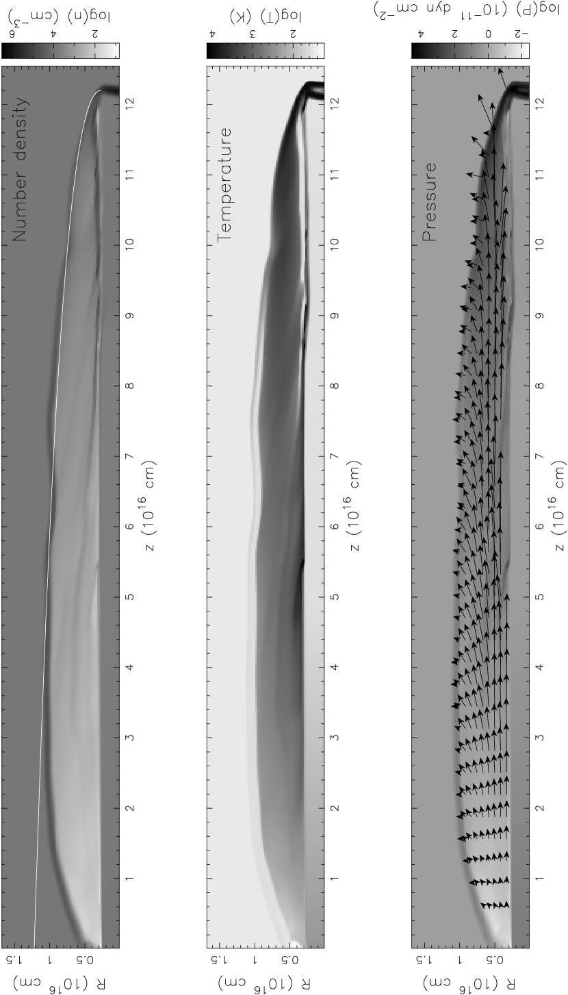
Figure 1:

Figure 2:

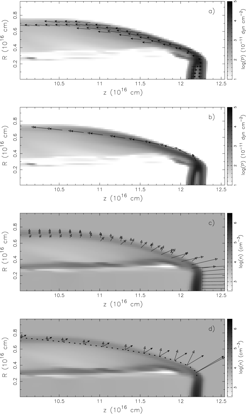
Figure 3:

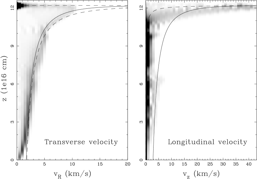
Figure 4:

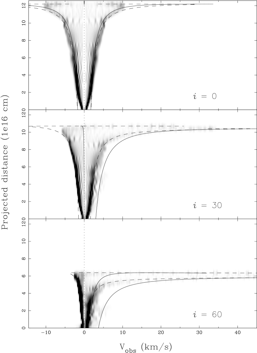
Figure 5:

Figure 6:

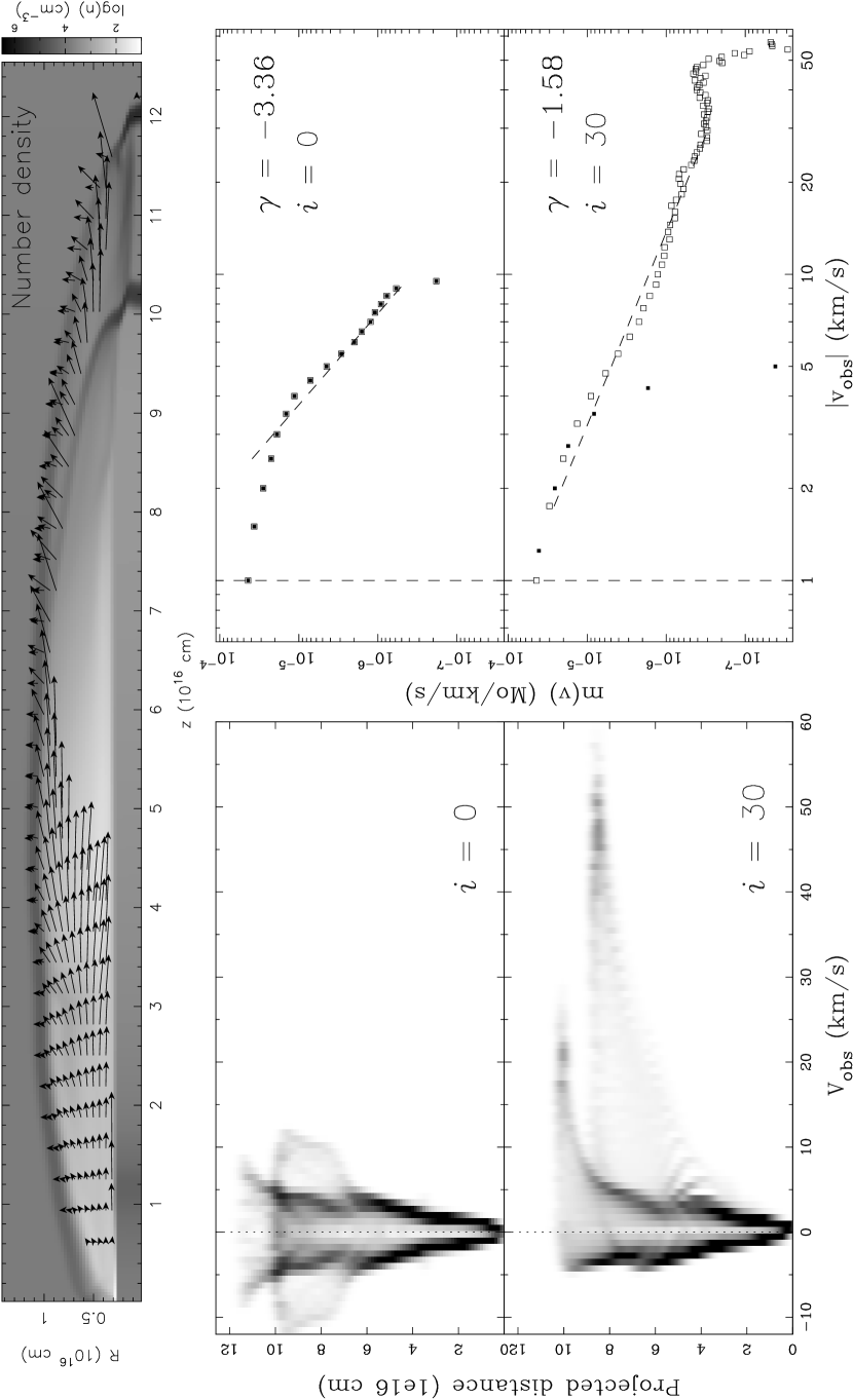
Figure 7:

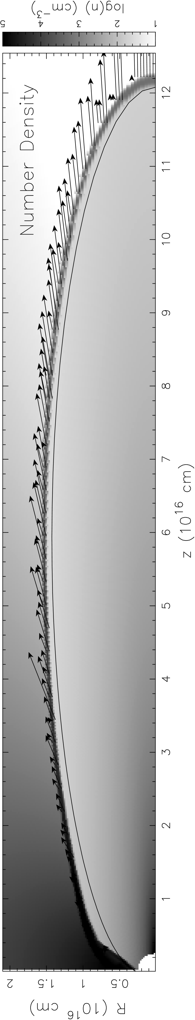
Figure 8:

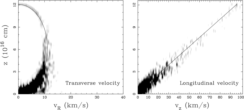
Figure 9:

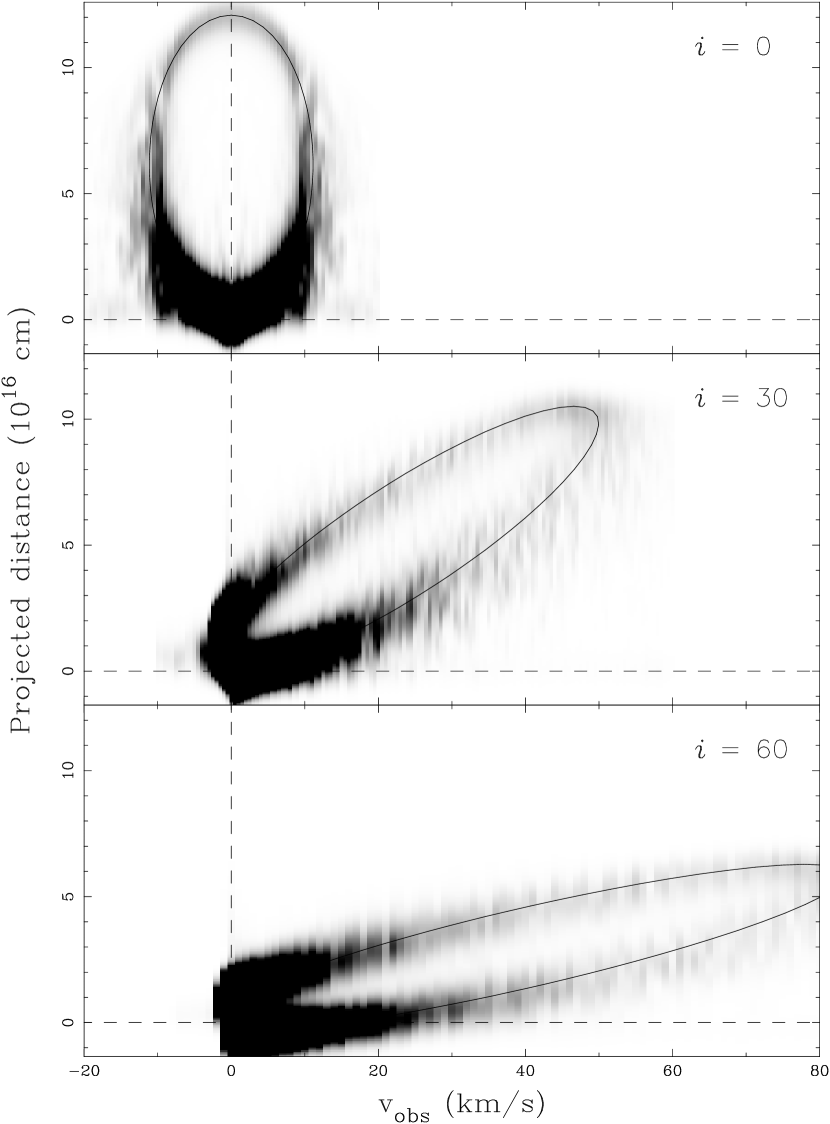
Figure 10:

Figure 11:

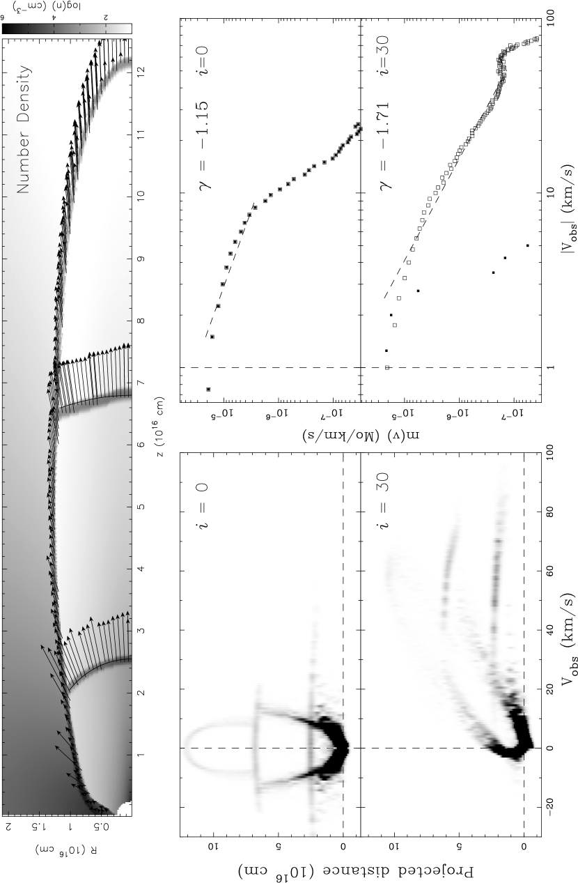
Figure 12:

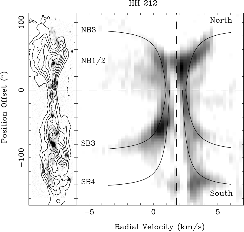
Figure 13:

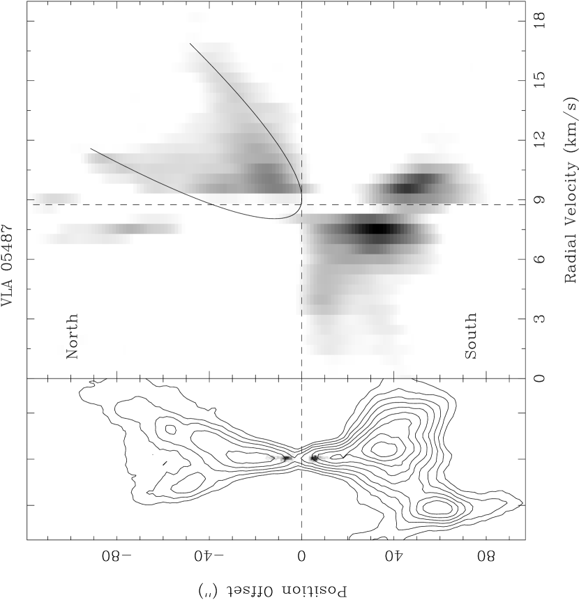
Figure 14:

References

- Anglada (1995) Anglada, G. 1995, Revista Mexicana de Astronomia y Astrofisica Conference Series, 1, 67
- Bachiller (1996) Bachiller, R. 1996, ARAA, 34, 111
- Bachiller et al. (1995) Bachiller, R., Guilloteau, S., Dutrey, A., Planesas, P. & Martin-Pintado, J. 1995, A&A, 299, 857
- Biro & Raga (1994) Biro, S. and Raga, A. C. 1994, ApJ, 434, 221
- Blondin, Konigl & Fryxell (1989) Blondin, J. M., Konigl, A. and Fryxell, B. A. 1989, ApJ, 337, L37
- Blondin, Fryxell & Konigl (1990) Blondin, J. M., Fryxell, B. A. & Konigl, A. 1990, ApJ, 360, 370
- Cabrit, Raga & Gueth (1997) Cabrit, S., Raga, A., Gueth, F. 1997, IAUS, 182, 163
- Chernin et al. (1994) Chernin, L.M., Masson, C.R., Gouveia dal Pino, E.M., Benz, W., 1994, ApJ, 426, 204
- Coppin, Davis, & Micono (1998) Coppin, K. E. K., Davis, C. J. & Micono, M. 1998, MNRAS, 301, L10
- Dalgarno & McCray (1972) Dalgarno, A. & McCray, R. A. 1972, ARA&A, 10, 375
- Davis et al. (2000) Davis, C. J., Berndsen, A., Smith, M. D., Chrysostomou, A.& Hobson, J. 2000, MNRAS, 314, 241
- de Gouveia dal Pino & Benz (1993) de Gouveia dal Pino, E. M. & Benz, W. 1993, ApJ, 410, 686
- Delamarter, Frank & Hartmann (2000) Delamarter, G., Frank, A. & Hartmann, L. 2000, ApJ, 530, 923
- Downes & Ray (1999) Downes, T. P. Ray, T. P. 1999, A&A, 345, 977
- Dutrey, Guilloteau & Bachiller (1997) Dutrey, A., Guilloteau, S. & Bachiller, R. 1997, A&A, 325, 758
- Frank & Mellema (1996) Frank, A. & Mellema, G. 1996, ApJ, 472, 684
- Fukui et al. (1993) Fukui, Y., Iwata, T., Mizuno, A., Bally, J., Lane, A.P. 1993 in Protostars and Planets III, ed. EH Levy, JI Lunine. Tucson; Univ. Ariz. Press
- Garnavich et al. (1997) Garnavich, P. M., Noriega-Crespo, A. , Raga, A. C. & Bohm, K. -H. 1997, ApJ, 490, 752
- Gueth & Guilloteau (1999) Gueth, F. & Guilloteau, S. 1999, A&A, 343, 571
- Gueth, Guilloteau & Bachiller (1996) Gueth, F., Guilloteau, S. & Bachiller, R. 1996, A&A, 307, 891
- Hollenbach (1997) Hollenbach, D. 1997, IAU Symp. 182: Herbig-Haro Flows and the Birth of Stars, 182, 181
- Hollenbach & McKee (1979) Hollenbach, D. & McKee, C. F. 1979, ApJS, 41, 555
- Lada (1985) Lada, C. J. 1985, ARA&A, 23, 267
- Lada & Fich (1996) Lada, C. J. & Fich, M. 1996, ApJ, 459, 638
- Lee et al. (2000) Lee, C.-F., Mundy, L.G., Reipurth, B., Ostriker, E.C., & Stone, J.M. 2000, ApJ, in press
- Li & Shu (1996a) Li, Z. -Y. & Shu, F. H. 1996a, ApJ, 468, 261
- Li & Shu (1996b) Li, Z. -Y. & Shu, F. H. 1996b, ApJ, 472, 211
- MacDonald & Bailey (1981) MacDonald, J. & Bailey, M. E. 1981, MNRAS, 197, 995
- Masson & Chernin (1992) Masson, C. R. & Chernin, L. M. 1992, ApJ, 387, L47
- Masson & Chernin (1993) Masson, C. R. & Chernin, L. M. 1993, ApJ, 414, 230
- Matzner & McKee (1999) Matzner, C. D. & McKee, C. F. 1999, ApJ, 526, L109
- McKee et al. (1982) McKee, C. F., Storey, J. W. V., Watson, D. M. & Green, S. 1982, ApJ, 259, 647
- Mellema & Frank (1997) Mellema, G. & Frank, A. 1997, MNRAS, 292, 795
- Meyers-Rice & Lada (1991) Meyers-Rice, B. A. & Lada, C. J. 1991, ApJ, 368, 445
- Micono et al. (1998) Micono, M., Davis, C. J., Ray, T. P., Eisloeffel, J. & Shetrone, M. D. 1998, ApJ, 494, L227
- Nagar et al. (1997) Nagar, N. M., Vogel, S. N., Stone, J. M. & Ostriker, E. C. 1997, ApJ, 482, L195
- Najita & Shu (1994) Najita, J. R. & Shu, F. H. 1994, ApJ, 429, 808
- Ostriker (1997) Ostriker, E. C. 1997, ApJ, 486, 291
- Ostriker (1998) Ostriker, E. C. 1998, Accretion Processes in Astrophysical Systems: Some Like it Hot!, 484
- Ostriker et al. (2000) Ostriker, E. C., Lee, C.-F., Stone, J.M. and Mundy, L.G. 2000, ApJ, submitted
- Raga & Cabrit (1993) Raga, A. & Cabrit, S. 1993, A&A, 278, 267
- Raga et al. (1990) Raga, A. C., Binette, L. , Canto, J. & Calvet, N. 1990, ApJ, 364, 601
- Ray, et al. (1996) Ray, T. P., Mundt, R. , Dyson, J. E., Falle, S. A. E. G. & Raga, A. C. 1996, ApJ, 468, L103
- Reipurth & Graham (1988) Reipurth, B. & Graham, J. A. 1988, A&A, 202, 219
- Reipurth & Olberg (1991) Reipurth, B. & Olberg, M. 1991, A&A, 246, 535
- Reipurth, Bally, & Devine (1997) Reipurth, B., Bally, J. & Devine, D. 1997, AJ, 114, 2708
- Reipurth et al. (1999) Reipurth, B., Yu, K. , Rodriguez, L. F., Heathcote, S. & Bally, J. 1999, A&A, 352, L83
- Richer et al. (2000) Richer, J. Shepherd, D., Cabrit, S., Bachiller, R., & Churchwell, E. 2000, in Protostars and Planets IV, ed. V. Mannings, A. P. Boss & S. S. Russell (Tucson: University of Arizona Press), in press
- Shang et al. (1998) Shang, H. , Shu, F. H. & Glassgold, A. E. 1998, ApJ, 493, L91
- Shu et al. (1991) Shu, F. H., Ruden, S. P., Lada, C. J. & Lizano, S. 1991, ApJ, 370, L31
- Shu et al. (1994) Shu, F. H., Najita, J., Ruden, S. P., & Lizano, S. 1994, ApJ, 429, 797
- Shu et al. (1995) Shu, F. H., Najita, J. , Ostriker, E. C. & Shang, H. 1995, ApJ, 455, L155
- Shu et al. (2000) Shu, F.H., Najita, J., Shang, H., & Li, Z. -Y. 2000, in Protostars and Planets IV, ed. V. Mannings, A. P. Boss & S. S. Russell (Tucson: University of Arizona Press), in press
- Smith, Suttner, & Yorke (1997) Smith, M. D., Suttner, G. & Yorke, H. W. 1997, A&A, 323, 223
- Stahler (1994) Stahler, S. W. 1994, ApJ, 422, 616
- Stone & Norman (1992) Stone, J. M. & Norman, M. L. 1992, ApJS, 80, 753
- Stone & Norman (1993a) Stone, J. M. & Norman, M. L. 1993, ApJ, 413, 198
- Stone & Norman (1993b) Stone, J. M. and Norman, M. L. 1993, ApJ, 413, 210
- Stone & Norman (1994) Stone, J. M. & Norman, M. L. 1994, ApJ, 420, 237
- Suttner et al. (1997) Suttner, G., Smith, M. D., Yorke, H. W. & Zinnecker, H. 1997, A&A, 318, 595
- Vlker et al. (1999) Vlker , R. , Smith, M. D., Suttner, G. & Yorke, H. W. 1999, A&A, 343, 953
- Yu, Billawala & Bally (1999) Yu, K. , Billawala, Y. & Bally, J. 1999, AJ, 118, 2940
- Zhang & Zheng (1997) Zhang, Q. & Zheng, X. 1997, ApJ, 474, 719
- Zinnecker, McCaughrean, & Rayner (1998) Zinnecker, H., McCaughrean, M. J. & Rayner, J. T. 1998, Nature, 394, 862