Cluster correlations in redshift space

Abstract

We test an analytic model for the two-point correlations of galaxy clusters in redshift space using the Hubble Volume N-body simulations. The correlation function of clusters shows no enhancement along the line of sight, due to the lack of any virialised structures in the cluster distribution. However, the distortion of the clustering pattern due to coherent bulk motions is clearly visible. The distribution of cluster peculiar motions is well described by a Gaussian, except in the extreme high velocity tails. The simulations produce a small but significant number of clusters with large peculiar motions. The form of the redshift space power spectrum is strongly influenced by errors in measured cluster redshifts in extant surveys. When these errors are taken into account, the model reproduces the power spectrum recovered from the simulation to an accuracy of $15\%$ or better over a decade in wavenumber. We compare our analytic predictions with the power spectrum measured from the APM cluster redshift survey. The cluster power spectrum constrains the amplitude of density fluctuations, as measured by the linear rms variance in spheres of radius $8h^{-1}$Mpc, denoted by $\sigma_{8}$. When combined with the constraints on $\sigma_{8}$ and the density parameter $\Omega$ derived from the local abundance of clusters, we find a best fitting cold dark matter model with $\sigma_{8}\approx 1.25$ and $\Omega\approx 0.2$, for a power spectrum shape that matches that measured for galaxies. However, for the best fitting value of $\Omega$ and given the value of Hubble’s constant from recent measurements, the assumed shape of the power spectrum is incompatible with the most readily motivated predictions from the cold dark matter paradigm.

1 Introduction

Rich clusters of galaxies are unique tracers of the large scale structure of the Universe. This is due to a number of reasons. First, clusters are the most massive virialised systems in place at any given epoch, occupying a special place at the head of the structure hierarchy. Second, although rich clusters are rare objects they are also bright, containing many luminous galaxies and emitting copious amounts of X-rays. Third, a cosmologically interesting volume of the universe can be surveyed much more rapidly using clusters than with galaxies, as a result of the huge difference in the number of redshifts that are required to be taken. Finally, the key reason for the utility of clusters is that it is far easier to interpret the observed properties of the cluster distribution in the context of theoretical models than is the case for galaxies.

There are three main statistical properties of the cluster distribution that have been used to place constraints upon the parameters of structure formation models. The first of these is the local abundance of rich clusters, which, as a consequence of their rarity, is extremely sensitive to the amplitude of density fluctuations on a scale that encloses the mass of a typical rich cluster before collapse (White, Efstathiou & Frenk 1993). The rate at which the abundance of clusters evolves with redshift further constrains the mass density of the universe (Eke, Cole, Frenk & Henry 1998; Blanchard et al. 1998). The second test is the distribution of cluster peculiar motions, which depends on the value of the mass density parameter $\Omega$, for models with similar mass fluctuation amplitudes (Croft & Efstathiou 1994b; Bahcall, Cen & Gramann 1994). Lastly, the spatial correlations of clusters constrain both the shape and amplitude of the power spectrum of the underlying dark matter (Mo, Jing & White 1996).

The latter of these, the clustering of clusters, is by far the best studied and, at the same time, the most controversial. The first measurements of the spatial two-point correlation function of Abell clusters demonstrated a much stronger clustering amplitude than that found for galaxies (Bahcall & Soneira 1983; Klypin & Kopylov 1983). Moreover, the clustering amplitude was found to increase significantly as the cluster number density decreased (Bahcall & West 1992). However, the exact correlation amplitude of clusters remains the subject of intense debate (Efstathiou et al. 1992; Miller et al. 1999). The early redshift surveys drawn from the Abell catalogue showed a significant enhancement of the clustering signal along the line of sight (Bahcall & Soneira 1983; Postman, Huchra & Geller 1992). Bahcall, Soneira & Burgett (1986) found that the clustering in the line of sight direction is consistent with a “velocity broadening” of $2000{\rm kms}^{-1}$, which they interpreted as arising from a combination of peculiar motions and geometrical distortions of superclusters.

Confronted by these results, several authors have argued that the Abell catalogue is afflicted by the superposition of clusters and that the clustering signal along the line of sight is artificial (Sutherland 1988; Sutherland & Efstathiou 1991; see also Lucey 1983). This prompted the construction of more objectively defined cluster catalogues drawn from machine-scanned survey plates with better calibrated photometry (APM: Dalton et al. 1992, 1994, 1997; Cosmos: Lumsden et al. 1992). The typical radius used to define clusters in the machine based catalogues is significantly smaller than that used by Abell, reducing the enhancement of cluster richness by projection effects. The clustering signal found in these more recent cluster redshift surveys does not display large enhancements along the line of sight; furthermore, the trend of increasing correlation amplitude with decreasing space density of clusters is weaker than that found for Abell clusters (Croft et al. 1997). A similar dependence of correlation length on cluster space density is found for the X-ray Bright Abell Cluster Sample, which is much less susceptible to line of sight projection effects than the optically selected Abell catalogue (Abadi, Lambas & Muriel 1998, Borgani et al. 1999). This result was recently confirmed using the REFLEX survey in a work by Collins et al. (2000), who found that there is no significant dependence of the clustering amplitud on the limiting flux, or equivalently on the space density of galaxy clusters.

Miller et al. (1999) counter these objections by pointing out that the early redshift surveys of Abell clusters contained large fractions of low richness clusters (Abell richness class $R=0$), that were not intended to form complete samples for use in statistical analyses. Furthermore, many cluster positions were determined by a single galaxy redshift. Miller et al. (1999) present the clustering analysis of a new redshift survey of Abell clusters with richness $R\geq 1$, and with the majority of cluster positions determined using several galaxy redshifts. The clustering signal along the line of sight is greatly reduced in the new redshift surveys compared with the Bahcall & Soneira (1983) results, and is comparable to the amount of distortion of the clustering pattern found for APM clusters (see Fig 5 of Miller et al. 1999). The anisotropy is further reduced after the orientation of two superclusters that are elongated along the line of sight is changed. Peacock & West (1992) also found that restricting attention to higher richness Abell clusters removed the strong radial anisotropy seen in the clustering measured in the earlier surveys.

It is clearly important to establish exactly what influence peculiar motions have on the inferred spatial distribution of rich clusters. In most previous theoretical studies, redshift space distortions have either been ignored or treated in a very approximate fashion. Quite often, redshift space distortions are modelled by simply assuming a boost to the clustering signal measured in real space, as predicted by Kaiser (1987). This effect arises from coherent flows on large scales where linear perturbation theory is applicable. However, if the peculiar motions of clusters are significant, then a damping of the clustering signal is expected on small scales. The transition between these two extreme types of behaviour needs to be modelled.

Computer simulations of structure formation through the gravitational amplification of small primordial fluctuations have been used extensively to model the spatial distribution of clusters (e.g. White et al. 1987; Bahcall & Cen 1992; Croft & Efstathiou 1994a; Watanabe, Matsubara & Suto 1994; Eke et al. 1996a). These early studies do not reach a consensus on the predicted clustering of clusters in cold dark matter cosmologies. Part of the reason for this discrepancy is due differences in the way in which clusters are identified in the simulations (Eke et al. 1996a). A further issue is the relatively small simulation volumes used and the small numbers of clusters analysed.

Recently, it has become possible to simulate much larger volumes than were used in these earlier studies, with sufficient resolution to allow the reliable extraction of massive dark matter haloes that can be identified as rich clusters (Governato et al. 1999; Colberg et al. 2000). In this paper, we analyse the redshift space clustering of massive dark matter haloes in the Hubble Volume simulations, the largest cosmological simulations to date, which are described in Section 2.1. This extends the comparison carried out by Colberg et al. (2000), who measured clustering in real space and compared the results with the predictions of analytic models. We outline the analytic model that we employ to predict clustering in redshift space in Sections 2.2 and 2.4. The distribution of cluster peculiar velocities in the simulations, an important ingredient of the analytic model for redshift space clustering, is analysed in Section 2.3. The predictions of the analytic model are confronted with measurements of clustering in the APM Cluster redshift survey in Section 3. We compare to cluster power spectrum data directly rather than to estimates of the correlation length. This avoids uncertainties introduced by the method used to derive a correlation length from the data. Moreover, the cluster power spectrum on large scales has the same shape as the power spectrum of the dark matter, as demonstrated in real space by Colberg et al. (2000), and, as we show in Section 2.4, is also the case under certain conditions in redshift space. We discuss our results and the constraints on cosmological parameters from the power spectrum of clusters in Section 4.

2 Theoretical predictions for the cluster power spectrum

2.1 N-body simulations

We compare analytic predictions of the statistical properties of cluster samples with measurements made from the Virgo Consortium’s “Hubble Volume” simulations. The simulations follow the evolution of Cold Dark Matter density fluctuations in two cosmologies: $\tau$CDM (with cosmological parameters $\Omega=1$, a power spectrum shape defined by $\Gamma=0.21$, following the parameterisation given by Efstathiou, Bond & White (1992), and a rms linear variance on a scale of $8h^{-1}$Mpc of $\sigma_{8}=0.6$) and $\Lambda$CDM (with $\Omega_{0}=0.3$, a cosmological constant $\Lambda_{0}c^{2}/(3H_{0}^{2})=0.7$, a power spectrum described by an effective shape parameter of $\Gamma=0.17$ and $\sigma_{8}=0.9$). The huge volume of the simulations ($8h^{-3}{\rm Gpc}^{3}$ for $\tau$CDM and $27h^{-3}{\rm Gpc}^{3}$ for $\Lambda$CDM) and the large number of particles employed ($10^{9}$) allow cluster statistics to be studied with unprecedented accuracy (Colberg et al. 2000; Jenkins et al. 2001). Dark matter haloes are identified using a friends-of-friends algorithm with a standard linking length (see Jenkins et al. 2001). The halo peculiar velocity is the peculiar motion of the centre of mass.

2.2 Clustering in real space

In this section we review the formalism employed to model the power spectrum of clusters using positions measured in real space, i.e. ignoring any distortion to the power spectrum arising from the peculiar motions of clusters. For further details, we refer the reader to the more complete discussions of this framework given, for example, by Mo & White (1996), Mo, Jing & White (1996), Borgani et al. (1997), Colberg et al (2000) and Moscardini et al (2000). Moscardini et al. (2000) also consider the evolution of clustering along the observer’s past light cone, an effect that we shall ignore for the relatively shallow observational sample studied in this paper.

Throughout this paper, we consider cluster samples that are defined by a characteristic spatial separation, $d_{c}$, or equivalently, by a space density $n$, where $d_{c}=1/n^{1/3}$. Such a sample is constructed by first ranking the clusters in order of mass, and then, starting from the most massive cluster, including progressively less massive clusters until the required space density is achieved.

We assume that on large scales, the real space power spectrum of the cluster sample, $P_{c}(k)$, can be related to the power spectrum of the underlying dark matter distribution, $P(k)$, by an effective bias factor, $b_{\rm eff}$, that is independent of scale:

$$P_{c}(k)=b^{2}_{\rm eff}P(k).$$ (1)

Colberg et al (2000) use the Hubble Volume N-body simulations to demonstrate that this is an excellent approximation over a decade in wavenumber, $0.01h{\rm Mpc}^{-1}<k<0.1h{\rm Mpc}^{-1}$. The task of computing the real space power spectrum of clusters can therefore be broken down into two steps: (i) The calculation of the appropriate power spectrum of the dark matter distribution, $P(k)$, taking into account non-linear evolution of density fluctuations. (ii) The computation of the linear bias factor, $b_{\rm eff}$, for clusters of a given abundance.

The first stage in the calculation is carried out using the prescription for transforming a linear theory power spectrum into a non-linear power spectrum described by Peacock & Dodds (1996). The transformation depends upon the cosmological parameters $\Omega$ and $\Lambda$, and upon the epoch or normalisation of the linear theory power spectrum. The formula given by Peacock & Dodds agrees well with the non-linear evolution found in N-body simulations (Jenkins et al. 1998).

The effective bias is computed by taking a weighted average of the bias, $b(M)$, for haloes of mass $M$ over the cluster sample under consideration

$$b_{\rm eff}=\frac{\int_{M_{\rm lim}}^{\infty}b(M)\frac{{\rm d}n(M)}{{\rm d}M}{\rm d}M}{\int_{M_{\rm lim}}^{\infty}\frac{{\rm d}n(M)}{{\rm d}M}{\rm d}M},$$ (2)

where $M_{\rm lim}$ is the lower mass limit that defines the sample and ${\rm d}n/{\rm d}M$ is the space density of halos in the mass interval $M$ to $M+\delta M$ (e.g. Mo & White 1996; Governato et al. 1999). We adopt the analytic form for the mass function of dark matter haloes proposed by Sheth, Mo & Tormen (2001 - hereafter SMT). These authors put forward a modification to the theory of Press & Schechter (1974) in which the collapse of dark matter haloes is followed using an ellipsoidal rather than spherical model. The SMT mass function agrees well with the results of N-body simulations, although the most significant improvements over Press-Schechter theory are realised for lower mass haloes than we consider in this paper (SMT; Jenkins et al. 2001). Following the theory developed by Mo & White (1996), SMT also derive an expression for the bias factor of dark matter haloes (their equation 8) which we adopt in our calculations.

As reported by Colberg et al. (2000), the SMT formulae for the mass function and halo bias factor predict an effective bias that is in good agreement with the results obtained from the Hubble Volume simulations. The analytic predictions for the real space power spectrum of clusters with $d_{c}=30.9h^{-1}$Mpc are shown by the solid lines in the upper panels of Fig. 2. The discrepancy is largest for the $\Lambda$CDM model, in which case the analytic prediction for the real space power spectrum is $12\%$ higher than the measurement from the simulation.

2.3 Cluster peculiar velocities

Figure 1: The histograms show the distribution of line of sight pairwise peculiar velocities of clusters with $d_{c}=30.9h^{-1}$Mpc in the Hubble Volume simulations: (a) shows the results for $\tau$CDM and (b) for $\Lambda$CDM, as indicated in the legend. The lower panels show the distributions when a single cluster rms redshift error of $\delta v=500{\rm kms}^{-1}$ is included. The smooth curves show theoretical distributions plotted with the same variance in pairwise peculiar velocity that is measured from the simulations. In (a) and (b), solid lines show a Gaussian distribution, dashed lines show an exponential distribution in $|v_{12}|^{3/2}$, dotted lines are for an exponential distribution in $|v_{12}|^{7/4}$, and the dot-dashed lines show an exponential distribution in $|v_{12}|$. In the lower panels, the variance includes the redshift error described above, added in quadrature to the variance measured in the simulation. In (c) and (d) only the Gaussian distribution is plotted.

The gravitationally induced peculiar motions of clusters distort the pattern of clustering if cluster redshifts are used to infer their spatial distribution. The distribution of cluster peculiar motions is therefore a key ingredient in the theoretical prediction of clustering in redshift space, as discussed in the next section.

In Fig. 1(a) and (b), the histograms show the distribution of line of sight pairwise peculiar velocities, $f(v_{12})$, measured for clusters in the Hubble Volume simulations with $d_{c}=30.9h^{-1}$Mpc; (a) shows the distribution for the $\tau$CDM simulation and (b) shows the results for $\Lambda$CDM. The smooth curves show various analytic distributions plotted with the pairwise velocity dispersion that is measured in the simulations ($\sqrt{<v^{2}_{12}>}=532{\rm kms}^{-1}$ for clusters in the $\tau$CDM simulation and $\sqrt{<v^{2}_{12}>}=434{\rm kms}^{-1}$ for $\Lambda$CDM); the solid line shows a Gaussian distribution, the dashed line shows an exponential distribution in $|v_{12}|^{3/2}$, the dotted line shows an exponential distribution in $|v_{12}|^{7/4}$ and the dot-dashed line shows an exponential distribution in $|v_{12}|$ (full details of the functional forms of these distributions may be found in Padilla & Baugh 2001). The bulk of the distribution of cluster peculiar velocities is adequately described by a Gaussian. However, Fig. 1 illustrates that this is not the case for the high velocity tails of the distributions. Moreover, the best fitting distribution is not the same in each simulation. Padilla & Baugh (2001) show that the shape of the high velocity tail depends upon the degree of non-linear evolution of the density fluctuations. The distribution of peculiar velocities is therefore of interest in itself, being sensitive to the cosmological parameters $\Omega$ and $\sigma_{8}$, and to the power spectrum of density fluctuations (Croft & Efstathiou 1994b). These issues are explored in more detail using the Hubble Volume simulations and other N-body simulations by Padilla & Baugh (2001).

The histograms in the lower panels of Fig. 1 show the distribution of peculiar velocities after incorporating a single cluster rms redshift measurement error of $\delta v\approx 500{\rm kms}^{-1}$, appropriate for the Abell and APM cluster redshift surveys (Efstathiou et al. 1992). The resulting distributions are much broader and closer to Gaussian, as shown by the corresponding solid lines; in these cases the variance is given by the sum in quadrature of the variance measured in the simulation and the rms redshift error stated above. The redshift error dominates over the variance expected for gravitationally induced peculiar velocities for the models that we consider in this paper. We therefore make the approximation in subsequent calculations when comparing to APM data that the variance in the pairwise peculiar velocity, including errors, is fixed at $\sqrt{<v^{2}_{12}>}\sim 850{\rm kms}^{-1}$, regardless of the model being studied. This in turn implies a single particle rms peculiar velocity of $\sigma=\sqrt{<v^{2}_{12}>}/\sqrt{2}\approx 600{\rm kms}^{-1}$.

2.4 Clustering in redshift space - power spectrum

2.4.1 Analytic model

The distortion of the power spectrum measured in redshift space generally displays two forms. On large scales, the amplitude of the power spectrum is boosted due to coherent inflows into overdense regions and outflows from underdense volumes (Kaiser 1987). On small scales, randomised motions within virialised structures cause a damping of power (e.g. Peacock 1999). Simple models have been developed that describe the transition between this large and small scale behaviour (Peacock & Dodds 1994, Cole, Fisher & Weinberg 1995). These schemes have been shown to work reasonably well for dark matter in N-body simulations (Cole, Fisher & Weinberg 1995; Hoyle et al. 1999). In this section we test whether such models provide an accurate description of the redshift space power spectrum of clusters of galaxies; this is necessary as we do not expect to find virialised structures in the cluster distribution.

For scales that are still evolving according to linear perturbation theory, the power spectrum in redshift space is given by

$$P^{s}_{c}(k,\mu)=P_{c}(k)\left(1+\beta\mu^{2}\right)^{2},$$ (3)

where $P_{c}$ is the cluster power spectrum in real space, as defined by equation 1, $P^{s}_{c}(k)$ is the cluster power spectrum in redshift space, $\beta=f(\Omega)/b_{\rm eff}$ ($f(\Omega)$ is the logarithmic derivative of the fluctuation growth rate) and $\mu$ is the cosine of the angle between the wavevector $k$ and the line of sight (Kaiser 1987; see also the discussion of this result in Cole, Fisher & Weinberg 1994).

Heuristic schemes have been put forward that extend this model for the redshift space power spectrum down to small scales to include the effects of a random velocity dispersion, under the assumption that the velocities are uncorrelated with the density field:

$$P^{s}_{c}(k,\mu)=P_{c}(k)\left(1+\beta\mu^{2}\right)^{2}D(k\mu\sigma_{v}).$$ (4)

For the case of a Gaussian distributed velocity dispersion,

$$D(k\mu\sigma_{v})=\exp(-k^{2}\mu^{2}\sigma^{2}_{v}/2),$$ (5)

whilst for an exponential distribution (Ballinger, Peacock & Heavens 1996),

$$D(k\mu\sigma_{v})=\frac{1}{1+\left(k\mu\sigma_{v}\right)^{2}/2}.$$ (6)

The spherically averaged form of equation 4 for a Gaussian velocity dispersion is given by Peacock & Dodds (1994):

$$P^{s}_{cl}(k)=G(\beta,y)P_{cl}(k),$$ (7)

where the function $G(\beta,y)$ is given by

$$G(\beta,y) =\frac{\sqrt{\pi}}{8}\frac{{\rm{erf}}(y)}{y^{5}}[3\beta^{2}+4\beta y^{2}+4y^{4}]$$ (8)

$$-\frac{\exp(-y^{2})}{4y^{4}}[\beta^{2}(3+2y^{2})+4\beta y^{2}],$$

where $\beta=f(\Omega)/b_{\rm eff}$ and $y=k\sigma_{v}/(100{\rm kms}^{-1}{\rm Mpc}^{-1})$. Errors in the determination of the cluster redshifts can be incorporated into this model by adding the redshift error in quadrature to the rms peculiar velocity to redefine $\sigma_{v}$. On the scales that we consider, there is effectively no difference in the distortion to the power spectrum when a Gaussian or exponential distribution of velocity dispersion is adopted (see Fig. 3 of Ballinger, Heavens & Peacock 1996).

2.4.2 Comparison with simulation results

Figure 2: The upper two panels show the real and redshift space power spectra for clusters with $d_{c}=30.9h^{-1}$Mpc; the left panels show the results for $\tau$CDM and the right panels show results for $\Lambda$CDM. The lines show analytic predictions and the symbols show measurements made directly from the simulations. Real space quantities are shown by solid lines and squares. The redshift space power spectrum measured in the simulations is shown by the circles. The dashed lines and triangles show the redshift space power spectrum after incorporating a redshift error into the determination of cluster positions. The lower panels show the ratio between redshift space and real space power spectra as a function of wavenumber. Again, points show the ratio for the measurements in the simulation. The circles show the ratio when only peculiar motions are considered, the triangles show the ratio when redshift errors are also included. The dashed line shows the analytic prediction of the ratio, when cluster redshift errors are included and should be compared with the triangles. The error bars are set by the number of modes per bin in wavenumber in the simulation.

The analytic prediction for the spherically averaged cluster power spectrum in redshift space is compared to the measurements from the Hubble Volume simulations in Fig. 2. In the simulations, the clustering pattern in redshift space is obtained by displacing clusters along the x-axis by an amount $\delta x=v_{x}/H_{0}$, where $v_{x}$ is the x-component of a cluster’s peculiar motion. The power spectrum of clusters in the Hubble Volume simulation is computed using the technique described in detail by Jenkins et al. (1998), and is equivalent to employing a very high resolution grid to perform the Fast Fourier Transform (FFT). Therefore, the scheme used to assign clusters to the FFT grid does not influence the recovered power spectrum.

The lower panels in Fig. 2 show the ratio of the redshift space to real space power spectrum as a function of wavenumber. The dashed lines show the outcome of dividing the analytic prediction for the real space spectrum into the prediction for the redshift space power spectrum, calculated including the effects of cluster redshift errors. At small wavenumbers (large scales) the ratios are in excellent agreement with the expectations from equation 3, which, using the approximation $f(\Omega)\approx\Omega^{0.6}$ predicts a ratio of $1.22$ for clusters in $\tau$CDM and $1.15$ in the $\Lambda$CDM simulation. Note the latter value changes by less than $1\%$ if the weak influence of a non-zero cosmological constant on $f(\Omega)$ is taken into account (Lahav et al. 1991). At high wavenumbers (small scales) we find that there is no damping of the power spectrum measured in redshift space when redshift errors are ignored. The analytic model reproduces the boost in power on large scales but predicts too much damping in the power on small scales. If an error is included in the cluster redshifts, then the model predicts the same form of distortion found in the simulations. The upper panels of Fig. 2 show that in this case, the analytic model for the redshift space power spectrum agrees with the simulation results to $15\%$ or better over the wavenumber range $-2<\log(k/h{\rm Mpc}^{-1})<-1$.

Further insight into the form of the distortion of the redshift space power spectrum caused by cluster motions can be obtained by plotting the power spectrum as a function of wavenumber perpendicular ($k_{\perp}$) and parallel ($k_{||}$) to the line of sight, $P(k_{\perp},k_{||})$, where $k=\sqrt{k^{2}_{\perp}+k^{2}_{||}}$ and $\mu=k_{||}/k$. We plot $P(k_{\perp},k_{||})$ for $d_{c}=30.9h^{-1}{\rm Mpc}$ clusters in the $\tau$CDM Hubble Volume simulation in Fig. 3. The smooth lines show analytic predictions. The light solid lines show the real space power spectrum. In the upper panel, the heavy solid lines show the redshift space power spectrum. In the lower panel the heavy lines show the power spectrum in redshift space including the effects of redshift errors in the determination of cluster positions. Two contour levels are plotted; the innermost sets of contours show $P(k_{\perp},k_{||})=4.9\times 10^{4}h^{-3}{\rm Mpc}^{3}$ and the outermost set show $P(k_{\perp},k_{||})=1.2\times 10^{4}h^{-3}{\rm Mpc}^{3}$. On large scales, the analytic predictions are in excellent agreement with the measurements from the simulations, in real space and in redshift space. In redshift space, the power is enhanced on large scales in the $k_{||}$ direction, displacing the contour of fixed power to higher wavenumbers. On intermediate scales, the distortion of the power spectrum is extremely sensitive to how well cluster redshifts are measured. The magnitude of the error estimated in the redshifts of APM and Abell survey clusters dominates over the distortion due to the peculiar motions of the clusters. Therefore, on these scales, the boost in power given by equation 3 is a poor description of the power spectrum. Qualitatively, the analytic model reproduces the form of the redshift space distortion measured in the simulation. However, due to a small discrepancy on intermediate scales between the predicted real space power spectrum and the measurement from the simulation (of around $10\%$ in the amplitude of $P(k)$), the contours do not coincide on this plot.

Finally, we compare the shapes of the redshift space power spectrum of clusters and dark matter in the $\tau$CDM Hubble Volume simulation in Fig 4. The results for clusters include errors in the cluster redshift determination, as discussed above. This plot illustrates that the redshift space power spectrum predicted by the model is in very good agreement with that measured for the dark matter. The effective bias measured in redshift space, as deduced by taking the ratio of cluster and mass power spectra in redshift space, is somewhat lower than the bias measured in real space. However, the bias measured in redshift space is still independent of scale. A measurement of the cluster power spectrum on large scales in redshift space would therefore yield the shape of the mass power spectrum in redshift space.

Figure 3: The power spectrum as a function of wavenumber parallel $k_{||}$ and perpendicular $k_{\perp}$ to the line of sight. The smooth lines show theoretical predictions, the other lines show measurements from the $\tau$CDM Hubble Volume simulation. The light lines in both panels show the power spectrum in real space. In the upper panel, the heavy lines show the power spectrum when the peculiar motions of clusters are taken into account. In the lower panel, redshift errors in the cluster positions are included. The inner most set of contours show the wavenumbers for which the power is $4.9\times 10^{4}h^{-3}{\rm Mpc}^{3}$; the outermost set show $P(k_{\perp},k_{||})=1.2\times 10^{4}h^{-3}{\rm Mpc}^{3}$

Figure 4: A comparison of real and redshift space power spectra for $d_{c}=30.9h^{-1}$Mpc clusters and for dark matter in the $\tau$CDM simulation. Solid symbols and lines show real space quantities and open symbols and dashed lines show redshift space quantities. Squares show power spectra for the dark matter and circles show cluster power spectra. Redshift errors have been included in the redshift space power spectrum of clusters. The solid lines in the upper panel show the fits to the real-space CDM model for the mass and clusters, and the dashed lines show the same fits for redshift space. The lower panel shows the effective bias obtained by taking the square root of the ratio between cluster and mass power spectra, both in real space (solid points and lines) and in redshift space (open points, dashed line).

2.5 Clustering in redshift space - correlation function

A key statistic for cluster samples is the two point correlation function $\xi$, measured as a function of cluster separation parallel to the line of sight, $\pi$, and perpendicular to the line of sight, $\sigma$. Efstathiou et al. (1992) used this statistic to argue that cluster samples drawn from the Abell catalogue are contaminated by projection effects, leading to a spurious enhancement of the clustering signal along the line of sight. Previously, the two-point correlation function $\xi(\sigma,\pi)$ has been studied for more abundant clusters, using much smaller volume simulations than are considered in this paper (e.g. Eke et al. 1996a). The Hubble Volume simulations can be used to resolve once and for all the issue of exactly how much anisotropy is expected in the two point correlation function from redshift space distortions alone.

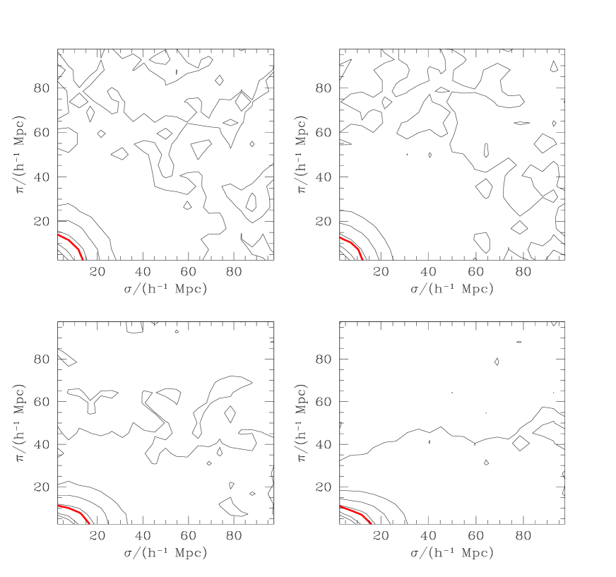
Figure 5: The two-point correlation function $\xi(\sigma,\pi)$ plotted in bins parallel ($\pi$) and perpendicular ($\sigma$) to the line of sight for $d_{c}=30.9h^{-1}$Mpc clusters in the $\tau$CDM (left-hand panels) and $\Lambda$CDM (right-hand panels) Hubble Volume simulations. The upper row shows the correlation function in real space and the lower row shows the redshift space correlation function. Contour levels are at $\xi=3,2,1,0.8,0.6,0.4,0.2$. The thick contour shows $\xi=1$.

In Fig 5, we show $\xi(\sigma,\pi)$ for clusters defined by $d_{c}=30.9h^{-1}$Mpc in the Hubble Volume simulations. The left hand panels show correlation functions measured in the $\tau$CDM simulation and the right hand panels show results for $\Lambda$CDM. The upper row of Fig. 5 shows the correlation function measured in real space and the lower row shows the redshift space correlation function. Note that in this Fig., we do not include any redshift errors. The contour levels are given in the figure caption; the thick contour shows $\xi=1$. As expected, the contours do not show any distortion when the correlation function is measured in real space. However, when the effects of peculiar motions are included, we find an apparent enhancement in the clustering signal perpendicular to the line of sight. This is a result of the flattening of the contours in the $\pi$ direction due to coherent flows in the cluster distribution. There is no evidence for any enhancement of the clustering signal along the line of sight. As a test, we have also measured $\xi(\sigma,\pi)$ for the dark matter in the Hubble Volume simulations, and in this case we do find a strong enhancement of the clustering amplitude in the $\pi$ direction on small scales. The relatively large separation of particles on the initial grid in the simulations ($3h^{-1}$Mpc in the case of $\Lambda$CDM) is therefore not an issue. The explanation of our result for clusters is that virialised structures have not had time to form in the cluster distribution.

The correlation function measured in the $\tau$CDM simulation is shown on an expanded scale in Fig. 6. In the lower panel, we include a rms cluster redshift error of $500{\rm kms}^{-1}$, in addition to the peculiar motions. When cluster redshift errors are included, a clear boost is evident in the amplitude of clustering parallel to the line of sight. It is interesting to note that the flattening of the contours due to coherent flows is no longer apparent; the magnitude of the cluster redshift errors is sufficient to obscure this effect. It can also be seen that the clustering amplitud along the $\sigma$ direction shortens noticeably. This can be explained as follows: the effect of the redshift errors on the correlation function at fixed values of $\sigma$, will be that of a smoothing function, which will take power from the scales corresponding to the higher correlations and transfer it to those of lower correlation. Therefore the value of $\xi(\sigma,\pi=0)$ will be smaller after the redshift errors are included, and the correlation lenght in the direction perpendicular to the line of sight will be shorter.

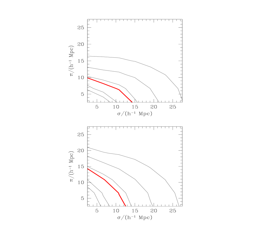
Figure 6: The two-point correlation function measured in redshift space for clusters in the $\tau$CDM simulation. The same contour levels used in Fig. 5 are plotted, with the thick contours showing $\xi=1$. In panel (a), gravitationally induced peculiar motions are considered. In (b), a rms cluster redshift error of $500{\rm kms}^{-1}$ is also included.

3 Comparison of the theoretical model with data

3.1 Clustering data

Figure 7: Testing the recovery of the power spectrum from the variance. The solid line shows a linear theory CDM power spectrum with $\sigma_{8}=1$ and $\Gamma=0.5$. The points show the power spectra recovered by applying equations 11 and 12 to the variance computed from the linear theory power spectrum (as given by equation 9). The different symbols denote the results obtained for different assumptions about the slope of the power spectrum.

Figure 8: (a) Estimates of the power spectrum of APM clusters inferred by applying equations 11 and 12 to the variance of counts in cells measured by Gaztañaga et al. (1995). The different symbols show the results for different assumptions about the slope of the power spectrum: the solid triangles use the slope of the variance data directly, the upwards pointing triangles are for a fixed value of $n=-1$ and the downwards pointing triangles are for $n=-0.5$. (b) A comparison of the power spectrum inferred using the counts-in-cells measurements of Gaztañaga et al. (1995) (filled triangles) with the direct measurement of the power spectrum of APM clusters by Tadros et al. (1998) (circles).

In this paper we compare the predictions of CDM models with the power spectrum measured from the APM cluster redshift survey. The data we consider are the variance of counts in cells measured by Gaztañaga, Croft & Dalton (1995) and the power spectrum measured by Tadros, Efstathiou & Dalton (1998). Both measurements were made using sample B of the APM cluster redshift survey, as defined by Dalton et al. (1994).

Before confronting the model predictions with these data, we first compare the two measurements with one another. The variance of counts in cells is given by an integral over the power spectrum multiplied by the Fourier transform of the window used to smooth the density field (e.g. Peacock 1999)

$$\sigma^{2}(R)=\frac{1}{2\pi^{2}}\int_{0}^{\infty}{\rm d}kk^{2}P(k)W^{2}(kR).$$ (9)

For a spherical top hat smoothing window of radius $R$,

$$W(kR)=\frac{3}{(kR)^{3}}\left(\sin(kR)-kR\cos(kR)\right).$$ (10)

The integral is reasonably sharply peaked around a characteristic wavenumber for a particular smoothing scale. Therefore, we make the approximation that the variance measured in a sphere of radius $R$ can be related to the power spectrum at a specified wavenumber (see Peacock 1991 who gives the result for a Gaussian smoothing window):

$$\sigma^{2}(R)=\Delta^{2}(k_{\rm eff}),$$ (11)

where $\Delta^{2}(k)=k^{3}P(k)/2\pi^{2}$. If we consider power law spectra, $P(k)\propto k^{n}$, then the effective wavenumber is defined as:

$$k_{\rm eff}=\frac{1}{R}\left[9I(n)\right]^{1/(n+3)},$$ (12)

Here $n$ is the logarithmic slope of the power spectrum at $k_{\rm eff}$, and the function $I(n)$ is defined by (see also Gaztañaga 1995):

$$I(n)=\int_{0}^{\infty}{\rm d}xx^{n-4}\left(\sin x-x\cos x\right)^{2}.$$ (13)

We demonstrate the accuracy of this transformation in Fig. 7. The points show the power spectra recovered by applying equations 11, 12 and 13 to the variance computed by integrating over the power spectrum shown by the solid line, which is our input spectrum (using equation 9). The different symbol types delineate the results obtained when different assumptions are made about the shape of the power spectrum. The most accurate answers are obtained when the shape of the power spectrum is inferred directly from the local slope of the variance. In this case, the recovered spectrum is at most $10\%$ below the correct value. The location of the turnover is reproduced when fixed values of the spectral index $n$ are used; however, the amplitude of the recovered spectrum can differ from that of the true spectrum by a factor of two, on scales larger than the turnover.

In Fig 8(a), we show estimates of the power spectrum made by applying equations 11 and 12 to the variance of counts in cells for APM clusters taken from Figure 3 of Gaztañaga et al. (1995). The different symbols show the results for different assumptions about the logarithmic slope of the power spectrum: the filled triangles show the power spectrum when the slope $n$ is estimated directly from the measured variance; the upwards pointing, open triangles show the results for a fixed value of $n=-1$ and the downwards pointing triangles show the case where $n=-0.5$. The power spectrum recovered in this way from the variance is robust to reasonable variations in the value of the spectral index adopted in equation 12.

We compare the power spectrum estimated from the variance of counts in cells, using the value of $n$ inferred from the data, with the power spectrum measured directly in redshift space by Tadros et al. (1998) in Fig 8(b). Over most of the range considered, the Tadros et al. (1998) result is approximately $50\%$ higher in amplitude than that obtained by Gaztañaga et al. (1995) Furthermore, though both measurements agree within the errors on the largest scales, the suggestion of a turnover seen in the Tadros et al. (1998) power spectrum is not as apparent in the power spectrum inferred from the variance data. In both papers the same sample of clusters was considered, with the same cuts applied in redshift. Both approaches make assumptions that could be partly responsible for the discrepancy. Tadros et al. (1998) need to specify a radial weighting scheme to obtain a minimum variance estimate of the power spectrum. The weighting scheme depends upon the power spectrum, but in practice the recovered spectrum is fairly insensitive to the value chosen. In addition, a random distribution of points with the same selection function as the cluster data is used to model the effects of the survey geometry on the recovered power spectrum. The measured power spectrum is sensitive to the level of smoothing applied to the selection function, though the tests presented by Tadros et al. (1998) suggest that the turnover found in the power spectrum is robust to changes in the smoothing. The Gaztañaga et al. (1995) approach does not require an estimate of the survey selection function (see Efstathiou et al. 1990), but does assume that the fluctuations are Gaussian. However, relaxing this assumption does not change the results significantly. Furthermore, the estimators used for the power spectrum and for the variance of counts in cells could respond in different ways to uncertainties in the mean density of clusters and to the irregular boundary of the APM survey.

3.2 Model parameters

We now compare theoretical predictions for the power spectrum of clusters in redshift space with measurements of the power spectrum of the APM cluster redshift survey. We make a number of assumptions in our model:

• We assume that primordial density fluctuations are Gaussian. The bulk of the available evidence suggests that any non-Gaussianity found in the distribution of large scale structure today is consistent with the gravitational evolution of an initially Gaussian density field (Moore et al. 1992; Gaztañaga 1994; Canavezes et al. 1998; Hoyle, Szapudi & Baugh 2000; Szapudi et al. 2000). Relaxing this assumption would affect the model predictions for the abundance of clusters and therefore, through changing the bias factor, the clustering of clusters (Robinson, Gawiser & Silk 2000).

• The dark matter in the universe is assumed to be cold dark matter.

• We assume that the shape of the dark matter power spectrum is the same as that measured for the galaxy power spectrum on the scales that we consider. Local biasing schemes yield an asymptotically constant bias on large scales between fluctuations in the galaxy and mass distributions (Coles 1993; see Cole et al. 1998 for realisations of this process). Observational support for this assumption is derived from the comparison of the power spectra of different types of object. Peacock & Dodds (1994) found that on large scales, the power spectra of optical galaxies, radio galaxies and clusters are consistent with a single underlying power spectrum after applying different, constant relative bias factors to the individual measurements. Tadros et al. (1998) also demonstrate that the power spectra of APM clusters and galaxies have the same shape on large scales and are related by a constant relative bias factor. The connection with the shape of the dark matter spectrum is made theoretically. Colberg et al. (2000) show that in real space the power spectrum of clusters is the same shape as the power spectrum of the underlying dark matter. In Section 2.4 we have demonstrated that the same conclusions hold in redshift space, when cluster redshift errors are included.

  The shape of the real space power spectrum of galaxies is well determined (Maddox et al. 1990; Baugh & Efstathiou 1993, 1994; Peacock & Dodds 1996; Gaztañaga & Baugh 1998). We adopt values of $\Gamma=0.2,0.25$, consistent with the recent determinations by Efstathiou & Moody (2001) and Eisenstein & Zaldarriaga (2001).

• We apply the methodology outlined in Section 2 and assume that the construction of a cluster sample specified by a space density is equivalent to taking all clusters above some mass threshold. To compare with sample B drawn from the APM cluster survey, we adopt a value of $d_{c}=30.9h^{-1}$Mpc.

Specifically, our model has two parameters:

• The cosmological density parameter, $\Omega_{0}$. We consider values in the range $\Omega_{0}=0.01-1$, with the condition that the model universe is spatially flat, i.e. if $\Omega<1$, then we adopt a cosmological constant, $\Lambda$, such that $\Omega+\Lambda c^{2}/(3H^{2})=1$. This is in agreement with the location of the first Doppler peak reported by the BoomeranG and Maxima cosmic microwave background experiments (Balbi et al. 2000; de Bernardis et al. 2000).

• The amplitude of density fluctuations, as specified by the linear rms variance in spheres of radius $8h^{-1}$Mpc, $\sigma_{8}$.

The theoretical models are computed for a mean cluster redshift of $z=0.083$, which is appropriate for APM sample B.

When comparing the model predictions with the data, we use the APM power spectrum results obtained for a cosmology with $\Omega=1$. Tadros et al. (1998) also compute the power spectrum of APM clusters in a background cosmology defined by $\Omega_{0}=0.2$, ${\Lambda_{0}c^{2}}/(3H^{2}_{0})=0.8$, and recover the same shape of power spectrum, but with an amplitude that is approximately $25\%$ higher. Therefore we make a systematic error when comparing data derived assuming $\Omega=1$ with a model in which a different value of $\Omega$ is adopted. To partially compensate for this, we take a pessimistic view of the errors on our theoretical predictions, adopting the level of the discrepancy found between the model and the $\Lambda$CDM simulation results of $15\%$.

3.3 Results

The theoretical models are assessed by computing a figure of merit:

$$\chi^{2}=\sum\left(P_{\rm model}(k)-P_{\rm data}(k)\right)^{2}/\left(\sigma^{2}_{\rm data}(k)+\sigma^{2}_{\rm model}(k)\right)$$ (14)

where the sum is over all the data points plotted in Fig 8(b) and we take $\sigma_{\rm model}(k)=0.15P_{\rm model}(k)$ (see Robinson 2000). We ignore any covariance between measurements of the power spectrum at different wavenumbers.

The results are shown in Fig. 9. The shaded regions show models that are within $\Delta\chi^{2}<1,4,9$ of the best fitting model when compared to the cluster power spectrum data indicated in the legend on each panel. The legend also gives the value of the power spectrum shape parameter, $\Gamma$, used in the models. In Fig. 9, the left hand panels show the results of the comparison to the Tadros et al. (1998) power spectrum data, and the right hand panels show the results using the power spectrum inferred from the Gaztañaga et al. (1995) measurement of the variance of APM clusters. The top row of the Fig. is for models with $\Gamma=0.2$, the bottom row is for $\Gamma=0.25$. We also plot the same $\Delta\chi^{2}$ contours for the constraint on the value of $\sigma_{8}$ derived from the abundance of hot X-ray clusters in the local universe by Eke, Cole & Frenk (1996b) (shown by the solid, dashed and dotted lines). The error on $\sigma_{8}$ quoted by these authors is $8\%$. The Eke et al. results agree with those from a recent reanalysis of the current cluster X-ray temperature data and of the theoretical framework of this constraint carried out by Pierpaoli, Scott & White (2000). The almost horizontal lines show the models in which clusters with a mean separation of $d_{c}=30.9h^{-1}$Mpc have effective bias factors of $b_{\rm eff}=1.5,2$ and $3$.

Figure 9: The constraints on the model parameters $\sigma_{8}$ and $\Omega_{0}$ from APM cluster power spectrum data. The shaded regions show contours of $\Delta\chi^{2}=1,4$ and $9$. The almost horizontal lines show parameter combinations for which the effective cluster bias is $b_{\rm eff}=1.5,2$ and $3$. The left hand panels show the outcome of comparing the models to the Tadros et al. (1998) power spectrum data, the right hand panels are obtained using the power spectrum inferred from the Gaztañaga et al. (1995) variance of counts in cells. The upper row is for models with $\Gamma=0.2$, the lower row for $\Gamma=0.25$. The lines show $\Delta\chi^{2}$ contours for the constraint on $\sigma_{8}$ and $\Omega_{0}$ from the local abundance of hot X-ray clusters and are reproduced in each panel (Eke, Cole & Frenk 1996b).

The $\Delta\chi^{2}$ contours derived from the cluster power spectrum constraint are almost parallel to the $\Omega$ axis, particularly for $\Omega>0.2$. Thus the amplitude of the cluster power spectrum in the models is determined largely by the value of $\sigma_{8}$ (see Mo, Jing & White 1996). The best fitting models with $\Gamma=0.25$ have a lower $\chi^{2}$ per degree of freedom than the $\Gamma=0.2$ models. The difference in the amplitude of the Tadros et al. (1998) and Gaztañaga et al. (1995) data is readily apparent from the shift in the location of the $\Delta\chi^{2}$ contours. The models that come closest to matching the Gaztañaga et al. (1995) data tend to have an effective cluster bias factor of $b_{\rm eff}\sim 2$, whilst the best fitting models for the Tadros et al. (1998) data tend to have $b_{\rm eff}\sim 1.5$.

The constraints on model parameters derived from the power spectrum data are much broader than those obtained from the abundance of rich clusters. Moreover, the shapes of the two sets of contours are different. A rough fit to the middle of the $\Delta\chi^{2}<1$ contour for the Gaztañaga et al. (1995) data, using models with $\Gamma=0.25$, yields $\sigma_{8}=\Omega_{0}^{-0.18+0.07(1-\Omega_{0})}$, whereas the cluster abundance constraint scaling is approximately $\sigma_{8}\propto\Omega^{-0.56}_{0}$.

We illustrate the consequences of an error in the space density of APM clusters in Fig. 10. The estimated space density is somewhat sensitive to the way in which the cluster selection function is normalised (Efstathiou et al. 1992). Furthermore, any projection effects that persist in the machine constructed catalogues could be responsible for moving poorer clusters into the sample. We therefore plot in Fig. 10 the constraints on model parameters assuming that $d_{c}=34h^{-1}$Mpc; this represents a $10\%$ error in $d_{c}$, corresponding to the space density of APM clusters being $30\%$ lower than assumed in Fig. 9. When the space density of the sample decreases, the minimum mass threshold that defines the sample increases, leading to larger effective bias parameters. The $\Delta\chi^{2}$ contours therefore shift down to lower values of $\sigma_{8}$.

Finally, we consider the constraints on the model parameters that are obtained when the two datasets, the cluster power spectrum and local abundance of hot X-ray clusters, are combined. In Fig. 11, we plot the $\Delta\chi^{2}$ contours after adding the $\chi^{2}$ values from comparing the model to the power spectrum data and to the observed cluster abundance. This operation assumes that the two datasets are independent. Due to the smaller errors, the cluster abundance constraint has the largest influence on the resulting $\chi^{2}$ contours. The vertical line on each panel shows the value of $\Omega$ that is consistent with the chosen $\Gamma$, given the recent determination of Hubble’s constant as $H_{0}=72\pm 8{\rm kms}^{-1}{\rm Mpc}^{-1}$ by Freedman et al. (2001), and assuming that $\Gamma=\Omega h$, where $H_{0}=100h{\rm kms}^{-1}{\rm Mpc}^{-1}$. The dotted lines indicate the range of values of $\Omega$ allowed following this prescription when the $1\sigma$ errors on Hubble’s constant are taken into account. The combined dataset favours low values of $\Omega$, with $\sigma_{8}=1$–$1.5$ for the Gaztañaga et al. measurement and $\sigma_{8}=1.6$–$2.3$ for the Tadros et al. power spectrum. In both cases, the shape of the power spectrum expected in the most easily motivated cold dark matter model, given the best fitting value of $\Omega$ is somewhat discrepant with the shape that we have assumed for the power spectrum; this disagreement is significant for the Tadros et al. data.

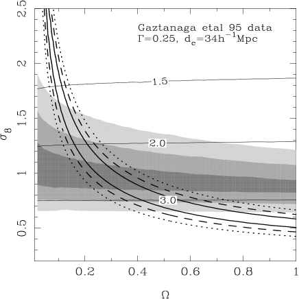
Figure 10: The constraints on model parameters when the abundance of APM clusters is reduced by $30\%$, so that $d_{c}=34h^{-1}$Mpc. The lines and shading are the same as for Fig 9.

Figure 11: The best fitting model parameters when the constraints from the cluster power spectrum and abundance measurements are combined. The contours show $\Delta(\chi^{2}_{P(k)}+\chi^{2}_{abun})=1,4$ and $9$. The top panel shows the $\Delta\chi^{2}$ contours when the Tadros et al. (1995) $P(k)$ is used and the bottom panel is for the Gaztañaga et al. (1995) data. A model power spectrum shape of $\Gamma=0.25$ is adopted and the model clusters are defined by $d_{c}=30.9h^{-1}$Mpc. The vertical line shows the value of $\Omega$ that is consistent with the adopted value of $\Gamma$, the CDM definition of $\Gamma=\Omega h$ and the measurement of Hubble’s constant by Freedman et al. (2001). The vertical dotted lines show the range of $\Omega$ permitted within the $1\sigma$ errors quoted on Hubble’s constant.

4 Discussion

The main goal of this paper was to establish the degree of distortion expected in the clustering pattern of rich clusters when viewed in redshift space. For this purpose, we undertook high precision measurements of the clustering of massive dark matter haloes, with the same space density as observational samples of clusters, using the largest extant cosmological simulations, the Virgo Consortium’s Hubble Volume simulations.

The rms peculiar motions of clusters in the Hubble Volume simulations are modest, of the order $300$–$350{\rm kms}^{-1}$ for a single cluster. Examples of pairwise velocity dispersions of the order of several thousand kilometers per second are found in the simulations, but are relatively rare. We find no evidence for any enhancement of the correlation amplitude along the line of sight arising from peculiar motions. The main type of distortion to the clustering pattern in redshift space is a flattening of the contours of $\xi(\sigma,\pi)$ due to coherent motions of clusters. The shape of the $\xi(\sigma,\pi)=1$ contour is remarkably similar to that found by Miller et al. (1999) for a recent survey of $R\geq 1$ Abell clusters (see their Fig. 7; we note however that lower amplitude contours in their Fig. still show some enhancement along the line of sight). If a redshift error is assigned to each cluster in the simulation (with a single cluster rms of $500{\rm kms}^{-1}$), then we reproduce the form of the distortion seen in measurements of $\xi(\sigma,\pi)$ from the APM cluster redshift survey, confirming that this survey is largely free from projection effects.

Similar conclusions were reached in a study of the redshift space distortions in the clustering of galaxies and groups in the Updated Zwicky Catalogue by Padilla et al. (2001). In this case, the groups are identified in three dimensions rather than in projection. A different set of issues need to be addressed when tuning a three dimensional group-finding algorithm, but superposition of groups along the line of sight should only occur for systems with high internal velocity dispersions. Padilla et al. (2001) found a strong enhancement in the line of sight clustering for galaxies. No such feature was detected in the correlation function of groups. These results were compared with predictions from N-body simulations, and the same form of distortion was found.

The analytic model outlined in Section 2 provides an accurate description of the redshift space power spectrum of clusters measured in Hubble Volume simulations, when errors in the cluster redshifts are included. We then compared the model predictions to the power spectrum measured from the APM cluster redshift survey in order to constrain the cosmological parameters $\Omega$ and $\sigma_{8}$. This is a more direct approach than a comparison with the cluster correlation length and thus avoids uncertainties regarding the way in which the correlation length is derived from the measured correlation function.

We have chosen to focus our attention on the APM cluster redshift survey, as this is the largest volume survey available that has been constructed from survey plates using a well specified, automated procedure. Miller & Batuski (2001) measure the power spectrum of a sample of $R\geq 1$ Abell clusters that does not display large enhancements in the line of sight clustering and which covers a larger volume than the APM survey. These authors find no evidence for a turnover in the cluster power spectrum and probe larger scales than the measurements of Gaztañaga et al. (1995) and Tadros et al. (1998). However, the space density of clusters in Miller & Batuski’s sample changes by a factor of two in a northern extension of the survey, which contributes much of the signal to the power spectrum measurement on large scales. Therefore more detailed modelling of the observational sample is required than we have attempted in this paper in order to make a realistic comparison with these data. Furthermore, the integrity of the Abell catalogue remains open to question, even for $R\geq 1$ clusters. Van Haarlem, Frenk & White (1997) demonstrated that mock Abell cluster catalogues constructed from N-body simulations suffer from significant incompleteness for $R\geq 1$ clusters. Power spectrum measurements have also been made using X-ray selected samples of clusters (e.g. Zandivarez, Abadi & Lambas 2001, Schuecker et al. 2001). Such samples have the appeal of greatly reducing projection effects as the X-ray emission is dominated by the high density core of a cluster’s dark matter halo. However, flux limited X-ray surveys mix clusters of different richness, so more careful modelling of the cluster selection is required to make robust theoretical predictions (Borgani et al. 1999; Moscardini et al. 2000).

We assume that the dark matter power spectrum has the shape measured for the galaxy power spectrum on large scales. This is a reasonable approximation if galaxy formation is a local process (Coles 1993; Cole et al. 1998). The model parameters that we vary to fit the cluster power spectrum data are then the cosmological density parameter $\Omega$ and the fluctuation amplitude $\sigma_{8}$. Within this scheme, the cluster power spectrum does not provide any constraint on $\Omega$ (see Mo, Jing & White 1996). The constraints on $\sigma_{8}$ are fairly broad as a result of the relatively large errors on the measured cluster power spectrum. This situation can be improved if additional information is used. Tadros et al. (1998) compare the power spectrum of galaxies and clusters in the APM survey and find that they have the same shape and can be related by a relative bias of $b\approx 1.8$. If one assumes that APM galaxies are essentially unbiased tracers of the dark matter on large scales (Gaztañaga 1994), then this additional constraint can be used to exclude models in which APM-like clusters have an effective bias that is very different from $b\sim 1.8$. However, we caution against the use of measurements of clustering in redshift space to restrict the value of an effective bias parameter in real space (see Fig. 4).

The range of acceptable model parameters is tightened considerably if the cluster power spectrum data is combined with measurements of the local abundance of rich clusters. The cluster abundance measurements themselves constrain the parameter combination $\sigma_{8}\Omega^{0.6}$ (White, Efstathiou & Frenk 1993). The constraint on these parameters from the power spectrum data has a different dependence on $\Omega$, thus allowing the degeneracy to be lifted. The best model parameters obtained using the combined data sets are $\sigma_{8}\approx 1.25$ and $\Omega\approx 0.2$. The best fitting value of $\Omega$ is inconsistent with the value suggested by our choice of $\Gamma$, if we use the most readily motivated prescription for setting the shape of the power spectrum in cold dark matter models, $\Gamma=\Omega h$, and adopt a recent measurement of Hubble’s constant by Freedman et al. (2001). The discrepancy is severest for the Tadros et al. (1995) power spectrum data (see the discussion of this data in Gawiser & Silk 1998). Whilst values of the shape parameter $\Gamma<\Omega h$ can be motivated physically by postulating a large baryon fraction or decaying neutrinos (Eisenstein & Hu 1998 ; White, Gelmini & Silk 1995), it is difficult to see how a value for $\Gamma$ that is much larger than $\Omega h$ could be accommodated. However, this situation could be alleviated if the abundance of APM clusters has been overestimated and a larger value of $d_{c}$ turns out to be more appropriate.

The cluster power spectrum data will improve significantly in the near future upon completion of the 2dF and SDSS galaxy redshift surveys (Colless 1999; York et al. 2000). Group catalogues will be constructed in three dimensions and the large volumes covered by the surveys mean that these catalogues will contain large numbers of clusters. Moreover, a comparison between the properties of clusters selected in projection and in redshift space will permit fine tuning of the two dimensional algorithms, that can then be applied to the deeper parent photometric catalogues.

References

- [] Abadi, M.G., Lambas, D.G., Muriel, H., 1998, ApJ, 507, 526.
- [] Bahcall, N.A., Cen, R.Y., 1992, ApJ, 398, L81.
- [] Bahcall, N.A., Cen, R.Y., Gramann, M., 1994, ApJ, 430, L13.
- [] Bahcall, N.A., Soneira, R.M., 1983, ApJ, 270, 20.
- [] Bahcall, N.A., Soneira, R.M., Burgett, W.S., 1986, ApJ, 311, 15.
- [] Bahcall, N.A., West, M.J., 1992, ApJ, 392, 419.
- [] Balbi, A., et al. , 2000, ApJ, 545, L1.
- [] Ballinger, W.E., Peacock, J.A., Heavens, A.F., 1996, MNRAS, 282, 877.
- [] Baugh, C.M., Efstathiou, G., 1993, MNRAS, 265, 145.
- [] Baugh, C.M., Efstathiou, G., 1994, MNRAS, 267, 323.
- [] Baugh, C.M., Gaztañaga, E. & Efstathiou, G., 1995, MNRAS, 274, 1049
- [] Blanchard, A., Bartlett, J.G., 1998, Astron. & Astroph., 332, L49.
- [] Borgani, S., Moscardini, L., Plionis, M., Gorski, K.M., Holtzman, J., Klypin, A., Primack, J.R., Smith, C.C., Stompor, R., 1997, New Astronomy, 1, 321.
- [] Borgani, S., Plionis, M., Kolokotronis, V., 1999, MNRAS, 305, 866.
- [] Canavezes, A., et al. , 1998, MNRAS, 297, 777.
- [] Colberg, J.M., et al. , 2000, MNRAS, 319, 209.
- [] Cole, S., Fisher, K.B., Weinberg, D.H., 1994, MNRAS, 267, 785.
- [] Cole, S., Fisher, K.B., Weinberg, D.H., 1995, MNRAS, 275, 515.
- [] Cole, S., Hatton, S.J., Weinberg, D.H., Frenk, C.S., 1998, MNRAS, 300, 945.
- [] Coles, P., 1993, MNRAS, 262, 1065.
- [] Colless, M., 1999, Phil. Trans. Roy. Soc. A., 357., 105.
- [] Collins, C.A., Guzzo, L., Boehringer, H., Schuecker, P, Chincarini, G., Cruddace, R., De Grandi, S, MacGillivray, H.T., Neumann, D.M., Schindler, S., Shaver, P., Voges, W., 2000, Astro-ph/0008245.
- [] Croft, R.A.C., Efstathiou, G., 1994a, MNRAS, 267, 390.
- [] Croft, R.A.C., Efstathiou, G., 1994b, MNRAS, 268, L23.
- [] Croft, R.A.C., Dalton, G.B., Efstathiou, G., Sutherland, W.J., Maddox, S.J., 1997, MNRAS, 291, 305.
- [] Dalton, G.B., Efstathiou, G., Maddox, S.J., Sutherland, W.J., 1992, ApJ, 390, L1.
- [] Dalton, G.B., Efstathiou, G., Maddox, S.J., Sutherland, W.J., 1994, MNRAS, 269, 151.
- [] Dalton, G.B., Maddox, S.J., Sutherland, W.J., Efstathiou, G., 1997, MNRAS, 289, 263.
- [] de Bernardis, P., et al. , 2000, Nature, 404, 955.
- [] Efstathiou, G., Bond, J.R., White, S.D.M., 1992, MNRAS, 258, 1P.
- [] Efstathiou, G., Dalton, G.B., Sutherland, W.J., Maddox, S.J., 1992, MNRAS, 257, 125.
- [] Efstathiou, G., Kaiser, N., Saunders, W., Lawrence, A., Rowan-Robinson, M., Ellis, R.S., Frenk, C.S., 1990, MNRAS, 247, 10P.
- [] Efstathiou, G., Moody, S.J., 2001, MNRAS submitted, astro-ph/0010478.
- [] Eisenstein, D., Hu, W., 1998, ApJ, 496, 605.
- [] Eisenstein, D., Zaldarriaga, M., 2001, ApJ, 546, 2.
- [] Eke, V.R., Cole, S., Frenk, C.S., 1996b, MNRAS, 282, 263.
- [] Eke, V.R., Cole, S., Frenk, C.S., Navarro, J.F., 1996a, MNRAS, 281, 703.
- [] Eke, V.R., Cole, S., Frenk, C.S., Henry, J.P., 1998, MNRAS, 298, 1145.
- [] Freedman, W.L., et al. , 2001, ApJ, in press, astro-ph/0012376
- [] Gawiser, E., Silk, J., 1998, Science, 280, 1405.
- [] Gaztañaga, E., 1994, MNRAS, 268, 913.
- [] Gaztañaga, E., Baugh, C.M., 1998, MNRAS, 294, 229.
- [] Gaztañaga, E., Croft, R.A.C., Dalton, G.B., 1995, MNRAS, 276, 336.
- [] Governato, F., Babul, A., Quinn, T., Tozzi, P., Baugh, C.M., Katz, N., Lake, G., 1999, MNRAS, 307, 949.
- [] Hoyle, F., Baugh, C. M., Shanks, T., Ratcliffe, A., 1999, MNRAS, 309, 659.
- [] Hoyle, F., Szapudi, I., Baugh, C. M., 2000, MNRAS, 317, L51.
- [] Jenkins, A., Frenk, C.S., Pearce, F.R., Thomas, P.A., Colberg, J.M., White, S.D.M., Couchman, H.M.P., Peacock, J.A., Efstathiou, G., Nelson, A.H., 1998, ApJ, 499, 20.
- [] Jenkins, A., Frenk, C.S., White, S.D.M., Colberg, J.M., Cole, S., Evrard, A.E., Couchman, H.M.P., Yoshida, N., 2001, MNRAS, 321, 372.
- [] Klypin, A.A., Kopylov, A.I., 1983, Soviet Astron. Lett., 9, 41.
- [] Lahav, O., Lilje, P.B., Primack, J.R., Rees, M.J., 1991, MNRAS, 251, 128.
- [] Lucey, J. R., 1983, MNRAS, 204, 33.
- [] Lumsden, S.L., Nichol, R.C., Collins, C.A., Guzzo, L., 1992, MNRAS, 258, 1.
- [] Kaiser, N., 1987, MNRAS, 227, 1.
- [] Maddox, S.J., Efstathiou, G., Sutherland, W.J., Loveday, J., 1990, MNRAS, 242, 43P.
- [] Miller, C.J., Batuski, D.J., Slingend, K.A., Hill, J.M., 1999, ApJ, 523, 492.
- [] Miller, C.J., Batuski, D.J., 2001, ApJ, in press, astro-ph/0002295.
- [] Mo, H.J., White, S.D.M., 1996, MNRAS, 282, 347.
- [] Mo, H.J., Jing, Y.P., White, S.D.M., 1996, MNRAS, 282, 1096.
- [] Moore, B., Frenk, C.S., Weinberg, D.H., Saunders, W., Lawrence, A., Ellis, R.S., Kaiser, N., Efstathiou, G., Rowan-Robinson, M., 1992, MNRAS, 256, 477.
- [] Moscardini, L., Matarrese, S., Lucchin, E., Rosati, P., 2000, MNRAS, 316, 283.
- [] Padilla, N.D., Baugh, C.M., 2001, in preparation.
- [] Padilla, N.D., Merchan, M.E., Valotto, C.A., Lambas, D.G., Maia, M.A.G., 2001, ApJ, in press, astro-ph/0102372.
- [] Peacock, J. A., 1991, MNRAS, 253, P1.
- [] Peacock, J. A., 1999, Cosmological Physics, Cambridge.
- [] Peacock, J. A. & Dodds, S. J., 1994, MNRAS, 267, 1020.
- [] Peacock, J. A. & Dodds, S. J., 1996, MNRAS, 280, L19.
- [] Peacock, J. A. & West, M.J., 1992, MNRAS, 259, 494.
- [] Pierpaoli, E., Scott, D., White, M., 2000, Mod. Phys. Lett. A., 15, 1357.
- [] Postman, M., Huchra, J.P., Geller, M.J., 1992, ApJ, 384, 404.
- [] Press, W.H., Schechter, P., 1974, ApJ., 187, 425.
- [] Robinson, J., 2000, astro-ph/0004023.
- [] Robinson, J., Gawiser, E., Silk, J., 2000, ApJ, 532, 1.
- [] Schuecker, P., et al. , 2001, Astron & Astroph., 368, 86.
- [] Sheth, R.K., Mo, H.J., Tormen, G., 2001, MNRAS, 323, 1
- [] Sutherland, W., 1988, MNRAS, 234, 159.
- [] Sutherland, W.J., Efstathiou, G., 1991, MNRAS, 248, 159.
- [] Szapudi, I., Branchini, E., Frenk, C.S., Maddox, S., Saunders, W., 2000, MNRAS, 318, L45.
- [] Tadros, H., Efstathiou, G., Dalton, G., 1998, MNRAS, 296, 995.
- [] van Haarlem, M.P., Frenk, C.S., White, S.D.M., 1997, 287, 817.
- [] Watanabe, T., Matsubara, T., Suto, Y., 1994, ApJ, 432, 17.
- [] White, M., Gelmini, G., Silk, J., 1995, Phys. Rev. D., 51, 2669.
- [] White, S.D.M., Efstathiou, G., Frenk, C.S., 1993, MNRAS, 262, 1023.
- [] White, S.D.M., Frenk, C.S., Davis, M., Efstathiou, G., 1987, ApJ, 313, 505.
- [] York, D.G., et al. , 2000, AJ, 120, 1579.
- [] Zandivarez, A., Abadi, M.G., Lambas, D.G., 2001, MNRAS, in press, astro-ph/0103378.