Deep near-IR observations of the Chandra Deep Field and of the HDF South

We present near-IR (J and Ks) number counts and colors of galaxies detected in deep VLT-ISAAC images centered on the Chandra Deep Field and Hubble Deep Field-South for a total area of 13.6 arcmin². The limiting surface brightness obtained is Ks$\simeq$22.8 mag/arcsec² and J$\simeq$24.5 (1$\sigma$) on both fields. A d$log$N/dm relation with a slope of $\sim 0.34$ in J and $\sim 0.28$ in Ks is found in both fields with no evidence of decline near the magnitude limit. The median J-Ks color of galaxies becomes bluer at magnitudes fainter than Ks$\sim 18$, in agreement with the different number counts slope observed in the two bands. We find a fraction ($\leq 5\%$ of the total sample) of sources with color redder than J-Ks=2.3 at magnitudes Ks$>20$. Most of them appear as isolated sources, possibly elliptical or dusty starburst galaxies at redshift $z>2$. The comparison of the observed number counts with models shows that our J-band and Ks-band counts are consistent with the prediction of a model based on a small amount of merging in a $\Omega=1$ cosmology. On the other hand, we fail to reproduce the observed counts if we do not consider merging independently of the parameters defining the universe.

1 Introduction

Near infrared (IR) observations provide significant advantages over optical ones in studying galaxy evolution because of the small and almost galaxy type independent k-corrections at these wavelengths and of their insensitivity to star formation activity over a wide redshift range (e.g. Cowie et al. 1994). They also provide a first guess about the stellar mass content of the galaxies since they trace the underlying old stellar population of galaxies out to $z\sim 2-3$. These are the main reasons why deep near-IR selected samples have been thought to provide constraints on the different galaxy formation and evolution scenarios.

When the first large IR detectors became available, near-IR galaxy counts were initially considered a powerful cosmological test (Cowie et al. 1990; Gardner et al. 1993). It was later realized that optical and near-IR observations were difficult to reconcile without number evolution (Broadhurst et al. 1992; Gronwall & Koo 1995; Babul & Rees 1992).

Disentangling the effects of luminosity and number density evolution is fundamental in understanding the nature of field galaxy formation and evolution allowing a direct comparison with models. For instance, hierarchical models, which assume that galaxies assemble through merging from smaller sub-units, make concrete predictions about the evolution of the merger rate, morphological mix and redshift distribution (e.g. Baugh et al. 1996; Kauffmann 1996; Kauffmann & Charlot 1998). In this scenario the number density of massive (and luminous in the near-IR) galaxies should decrease with increasing redshift. Consequently, an IR selected sample is better suited to investigate the density of these galaxies.

Kauffmann & Charlot (1998) suggest that the redshift distribution of a K-band selected sample can provide an observational test able to discriminate between hierarchical models and pure luminosity evolution (PLE) models. They show that hierarchical models predict a substantially lower fraction of high-$z$ galaxies at any redshift than do PLE models. Moreover, PLE models predict a high redshift tail of the redshift distribution of galaxies much more extended than in hierarchical models. Fontana et al. (1999) applied this test to a composite sample, deriving the photometric redshift distribution of galaxies down to K$<21$. They found only $\sim 5\%$ of galaxies at $z>2$ in good agreement with predictions of hierarchical models.

Near-IR colors have been used, e.g. by Eisenhardt et al. (2000), to select $z>1$ galaxies with the aim to constrain the fraction of high redshift galaxies in a K-band selected sample.

We have obtained deep J and Ks band VLT-ISAAC observations centered on the Chandra Deep Field ($\sim 6$ arcmin², CDF hereafter) and Hubble Deep Field South ($\sim 7.4$ arcmin², HDFS hereafter) which extend to J$\sim 24.5$ and Ks$\sim 23$. The HDFS data are in common with those of a similar proposal. This data set constitutes the widest area surveyed at these near-IR magnitude limits. In this paper we present counts and near-IR colors of galaxies detected in these two fields. The plan of the paper is as follows: in §2 we describe the observations and the data reduction and show in §3 the procedure adopted to construct our photometric samples and to derive number counts. In §4 we present color distributions and in §5 we compare the observed number counts with different models. In §6 we use color selection to identify $z>1$ and $z>2$ galaxies and to obtain lower limits to their number densities. Finally, in §7 we summarize our results and conclusions.

2 Observations and Data Reduction

2.1 Observations and Photometric Calibration

The data have been obtained with the ISAAC infrared imager/spectrometer (Moorwood et al. 1999) at the ESO VLT-UT1 telescope. ISAAC is equipped with a 1024$\times$1024 pixel Rockwell Hawaii array providing a plate scale of 0.147 arcsec/pix and a total field of view of about 2.5$\times$2.5 arcmin. The two observed fields are centered at 03h32m16s, -27^o47’25” the center of the Chandra Deep Field and at 22h32m55s, -60^o33’,08” the center of the Hubble Deep Field-South. The observations were gathered over several nights from September to December 1999 under homogeneous seeing conditions: around 0.6 arcsec in the case of the HDFS and around 0.7 arcsec in the case of the CDF. The CDF was imaged in the J and Ks bands while the HDFS in the Js, H and Ks bands (see Tab.1).

The standard “auto-jitter” mode was used to take all the images, with the telescope being offset by random amounts up to 30 arcsec (CDF) and 20 arcsec (HDFS) between individual short exposures. In Tab. 1 we summarize the number of frames and the relevant total exposure times in each band for the two observed fields.

Photometric calibration of the observations has been made by observing several standard stars from the list of Infrared NICMOS Standard Stars (Persson et al. 1998) with magnitudes ranging between 10 and 12. Instrumental total flux has been estimated by deriving the growth curve for each star using the IRAF task phot. The estimated magnitudes have then been corrected for atmospheric extinction assuming A_J=0.1, A_H=0.04 and A_Ks=0.05. The typical uncertainty in the derived photometric calibration ranges between 0.02 and 0.04 mag.

Filter	$\bar{\lambda}$	$\Delta\lambda$	Number of	texp	FWHM	$\mu$(1$\sigma$)
	($\mu$n)	($\mu$n)	frames	(s)	(arcsec)	mag/arcsec2
			CDF
J	1.25	0.26	67	12060	0.65	24.40
Ks	2.16	0.27	304	30400	0.70	22.85
			HDFS
Js	1.24	0.16	210	25200	0.59	24.55
Ks	2.16	0.27	487	29220	0.62	22.74

Table 1: Details of observations and image quality

2.2 Data reduction

Raw frames have been first corrected for bias and dark current pattern by subtracting a median dark frame. The flat field corrections have been made by using a mean differential sky-light flat obtained by averaging the difference between a set of low-count sky flat images from a set of high-count sky flat images.

Frames have been then processed by DIMSUM to produce the sky subtracted frames on the basis of the following recipe. A first pass of DIMSUM produces a “raw” final co-added image by which to derive a master mask frame flagging pixels belonging to sources. This master mask is de-registered to create a proper mask relevant to each frame. For each frame a sky background image is thus generated by averaging a set (from 3 to 6) of time adjacent frames where sources are now masked out. This procedure makes it possible to obtain sky subtracted frames where sources are not surrounded by dark halos typical of a sky subtraction process performed without masking objects.

The sky-subtracted frames have been then inspected and sky residuals were removed where present. Sky residuals have been modeled using the IRAF task imsurfit by fitting a bi-cubic spline to the frame after masking out the sources.

Frames have been then rescaled to the same airmass using the airmass information stored in the header of the images and to the same zeropoint by comparing the photometry of all the sources detectable in each frame. Finally, before shifting and co-adding, frames have been additively rescaled to the same median value.

Shifting and co-adding have been then performed with DIMSUM. The final co-added image is the average of the shifted frames. The quality of the final images is shown in Table 1 where the measured FWHM and the 1$\sigma$ limiting surface brightness are reported.

Figure 1: The figure compares the Ks-band counts obtained in this work in the CDF and in the HDFS with those in the literature. The Maihara et al. (2000) counts have been plotted down to their S/N$\sim$3 limit. The slope at Ks$>19$ is 0.28 both for the CDF and the HDFS Ks-band counts.

Figure 2: The J-band galaxy counts obtained in this work are compared with those in the literature. The Maihara et al. (2000) counts have been plotted down to their S/N$\sim$3 limit. Our counts continue to rise with a power law slope at J$>20$ of 0.37 and 0.34 in the CDF and the HDFS respectively.

3 Number Counts

3.1 Object catalogs and magnitudes

Object detection has been performed using the SExtractor package (Bertin and Arnouts 1996). We used a Gaussian function with a FWHM matching the one measured on the frames to convolve the image and an RMS weighting map to optimize the detection procedure. Since the two data sets have been obtained under slightly different seeing condition, we used different detection thresholds such that the faintest detectable source in both the fields has a minimum signal-to-noise ratio of S/N=3 over the seeing disk. The raw catalogs were then been cleaned of those objects having saturated pixels and/or lying too close to the edges to perform a reliable flux estimate.

The Ks-band selected catalogs thus obtained contain 332 sources over an area of 6.01 arcmin² (CDF) and 414 sources over 7.47 arcmin² (HDFS). The CDF near-IR catalog is available in electronic form via http://www.merate.mi.astro.it/$\sim$saracco. The multi-band HDFS catalog will be published in a forthcoming paper (Vanzella et al. 2001).

In order to establish the most reliable and unbiased estimate of the ”total” flux of sources in our images, we compared different magnitude estimates among them. We focused our attention on three different issues: 1) the magnitude which minimizes the systematic underestimate of the flux at faint magnitudes; 2) identifying the most reliable estimate of the flux of blended sources and 3) the best color estimate of the sources.

We made use of the simulated images to compute the completeness corrections to number counts (see §3.2) to systematically investigate these three different issues. The results of our analysis agree with those previously found by Martini (2000) and Saracco et al. (1999) showing that the SExtractor BEST magnitude (i.e. isophotal corrected magnitude for sources flagged by SExtractor as blended and Kron-like magnitude for the remaining sources) underestimates the flux when approaching the limits of the survey. This bias is much larger in the case of isophotal magnitudes (both corrected or not). We also found that a 2 arcsec aperture photometry ($\sim$3$\times$FWHM in our images) brightened by 0.15 mag (derived by point-like sources) gives a good estimate of the magnitude of the faintest sources while underestimate the flux of Ks$<$20.5 sources and fails to recover that of blended sources.

We thus estimated magnitudes on the basis of the following steps:

• the 2 arcsec aperture magnitude corrected by 0.15 mag was assigned to those “isolated” sources having an isophotal diameter (on the smoothed image) smaller than 2 arcsec.

• the BEST magnitude was assigned to the remaining sources.

This is very similar to the procedure adopted in the previous papers (Fontana et al. 2000; Arnouts et al. 1999)

3.2 Galaxy counts

To derive galaxy counts, we first removed stars from the samples relying on the Sextractor star/galaxy classifier. We defined stars as those sources having a stellarity index larger than 0.9 and a point-source FWHM in all the bands. A visual inspection made on the F814W band image of the HDFS confirmed the reliability of the classification. We found 16 and 23 stars (all of them brighter than Ks=21) in the CDF and in the HDFS respectively. The possibility that our classification fails to detect fainter stars implies negligible differences in the number counts at these magnitudes, since the surface density of stars is at least one order of magnitude lower than that of galaxies.

We have computed the correction factors for faint, undetected sources following the recipe described in Saracco et al. (1999) and Volonteri et al. (2000). We generated for each band a set of frames by dimming our final images by various factors and adding pure poissonian noise at the same level as that of the original images. Sextractor was then run with the same detection parameters to search for real sources in the dimmed frames. The correction factor $\bar{c}$ is the mean number of dimmed galaxy which should enter the fainter magnitude bin over the mean number of detected ones. In Tab. 2 we report the raw counts $n_{r}$, the correction factors $\bar{c}$, the counts per square degree corrected for incompleteness and their errors $\sigma_{N}$. Errors were obtained by quadratically summing the Poissonian contribution $\sigma_{n_{r}}=\sqrt{(}n_{r})$ of raw counts, and the uncertainty on the correction factor $\sigma_{c}$.

			CDF	6.01 arcmin2			HDFS	7.47 arcmin2
Ks	$n_{r}$	$\bar{c}$	N/mag/deg2	$\sigma_{N}$	$n_{r}$	$\bar{c}$	N/mag/deg2	$\sigma_{N}$
16.00	3	1	1198	1194	1	1	482	482
17.00	4	1	2396	1694	9	1	1928	1446
18.00	12	1	4193	1694	21	1	8193	2208
19.00	33	1	13180	4792	29	1	11566	2595
19.75	11	1	11980	3973	25	1	22168	5161
20.25	32	1	38340	6777	30	1	28916	5653
20.75	37	1	44330	7287	40	1	38554	6528
21.25	41	1	49120	7671	56	1	53976	7724
21.75	44	1	52710	7947	82	1	79036	9346
22.25	77	1.1	101500	1.103e+04	79	1.13	86043	10370
22.75	35	3.3	138400	1.288e+04	37	4.5	160482	28250
J	$n_{r}$	$\bar{c}$	N/mag/deg2	$\sigma_{N}$	$n_{r}$	$\bar{c}$	N/mag/deg2	$\sigma_{N}$
18.00	3	1	1445	1163	6	1	2409	1669
19.00	5	1	963	1339	10	1	3373	1894
19.75	8	1	2891	2726	15	1	11566	3732
20.25	17	1	5783	3974	13	1	9638	3475
20.75	15	1	10602	3732	16	1	13493	3855
21.25	18	1	17349	4089	26	1	23132	4914
21.75	41	1	39518	6171	39	1	37590	6019
22.25	49	1	47228	6746	48	1	46265	6677
22.75	59	1	56867	7403	87	1	82891	8990
23.25	93	1	89638	9295	91	1	87710	9194
23.75	86	1.3	134891	8938	133	1.1	141092	12300
24.25	70	2.5	207469	8064	86	2.1	174000	18938

Table 2: Differential number counts in the Ks-band and in the J-band derived on the CDF (upper panel) and on the HDFS (lower panel). Errors take into account the Poissonian error on raw counts and the uncertainties in the completeness correction factor $c$.

Fig. 1 and 2 show the number counts derived for the Ks-band and for the J-band, respectively. We do not find significant deviations between the CDF and HDFS. The counts follow a d$log$N/dm relation with a slope $\gamma_{J}\simeq 0.34$ at J$\geq 20$ and $\gamma_{K}\simeq 0.28$ at Ks$\geq 19$. Also plotted in the figures are number counts derived from the previous surveys taken from the literature.

The surface density of galaxies we derived as well as the rate at which it increases with apparent magnitude, i.e. the slope of the counts, lie in between those derived previously by other surveys.

The remarkable scatter among the surveys may be ascribed to the superposition of various effects: the slightly different filters (K, K’, Ks and J, Js), the different method used to estimate magnitudes, possible systematics in the photometric calibration and cosmic variance which could significantly affect the number counts at faint magnitudes where the area covered by the surveys is always narrower than few arcmin². It is actually at magnitudes fainter than K=21 and J=23 that the largest discrepancies among various surveys occur. Finally, fields centered on high-redshift target objects may result in a significant excess of the number counts (e.g. Soifer et al. 1994).

The CDF and HDFS Ks-band counts derived here are systematically lower than those of Bershady et al. (1998), Saracco et al. (1999) and McCracken et al. (2000). The largest discrepancy occurs with respect to Bershady’s counts (a factor 1.7 at Ks$\sim 22.5$) which increase faster (especially in the Ks band) with respect to our counts, the slope being $\sim 0.36$. Both Bershady et al. (1998) and McCracken et al. (2000) surveyed high Galactic latitude blank fields covering an area smaller than 2 arcmin². They count more than 200 and 80 objects down to K$\sim 23.5$ and K$\sim 22.5$ respectively. While Bershady et al. use fixed aperture magnitudes (within $\sim 2$ arcsec) corrected to total on the basis of the object size, McCracken et al. use a Kron-type magnitude. Saracco et al. (1999) surveyed an area of 20 arcmin² centered on the NTT Deep Field (Arnouts et al. 1999) and including the high-redshift quasar BR 1202-07. They detect $\sim 1000$ objects to a limiting magnitude K${}_{s}\sim 22.5$ and apply an aperture correction to the 2.5 arcsec fixed aperture magnitude. The method we used to estimate magnitudes is quite similar to the one used both by Bershady et al. and Saracco et al. The different surface density of galaxies they found with respect to the one here derived may thus be ascribed to cosmic variance affecting the small area covered by Bershady et al. and the field surveyed by Saracco et al. due to the presence of the high-redshift quasar. In the case of McCracken et al. data their different method used to estimate magnitudes adds to the high count fluctuations expected in such a small area.

On the other hand our counts, which agree with those of Moustakas et al. (1997), are systematically higher than those of Djorgovski et al. (1995) and of the recent very deep counts derived by Maihara et al. (2000) on the Subaru Deep Field (SDF). In particular the CDF and HDFS counts are in excess at magnitudes J$\geq 23$ and Ks$\geq 22$ with respect to the SDF counts which are described by a slope of $\sim 0.23$ and they are always $\sim 1.4$ times higher than those derived by Djorgovski et al. Bershady et al. (1998) claim that the corrected aperture magnitude used by Djorgovski et al. (1995) may result in an overestimation of the depth of their survey up to 0.5 mag.

It is worth noting that extrapolating the scaling relation found for field K-band selected galaxies (Roche et al. 1999) to Ks$\sim$21, we found that clustering can produce count fluctuations of $\sim 25\%$ in the magnitude range $20.5<Ks<21.5$ over an area comparable to the CDF and HDFS. These fluctuations rise up to $\sim 30-32\%$ over areas of 2-1 arcmin². Thus, large scale structure fluctuations alone could in principle account for most of the observed discrepancies among the surveys at faint magnitudes.

Figure 3: Color-magnitude diagram for the CDF Ks selected sample. Open circles represent galaxies detected both in the J and in the Ks band the arrows mark the J-Ks lower limits. The horizontal lines represent the typical J-K color of a main sequence M6 star (dashed line, J-K$\simeq 0.96$) and of an elliptical galaxy at $z\geq 2$ (solid line) respectively. The expected J-Ks color for a pure galaxy population of ellipticals (E, solid curve), spirals (Sb, long-dashed curve) and irregular (Irr, short-dashed curve) types is also shown (H₀, $q_{0}$ = 50, 0.5).

Figure 4: Same as Fig. 3 but for the HDFS sample

4 Colors of galaxies

The near-IR color of galaxies of our samples has been obtained by running SExtractor in the so-called double-image mode: J (Js) magnitudes for the Ks selected sample have been derived using the Ks frame as a reference image for detection and the J (Js) image for measurements. We used the difference between the 2 arcsec diameter aperture magnitudes ($\sim 3\times$FWHM) to estimate the color of isolated sources while the difference between isophotal magnitudes has been adopted to measure the color of blended sources. This is to minimize the uncertainties on flux estimates occurring for blended sources in the case of a fixed aperture magnitude. We considered genuine estimates those signals exceeding 2$\sigma$ above the background while fainter signals have been replaced by the 2$\sigma$ upper limit.

In Fig. 3 and 4 the color-magnitude diagrams of the Ks selected CDF and HDFS samples are shown respectively: open circles represent galaxies detected both in the J and in the Ks band while the lower limits to the J-Ks color are represented by the arrows. It is worth noting that the different depth reached in the J filters (see Tab. 1) gives rise to a difference of $\sim 0.15$ mag in the limiting J-Ks color between the two fields. Point-like sources are marked by star symbols. The median J-Ks color in 0.5 magnitude bins for our sample (filled circle) is also plotted and compared to the value given in Bershady et al. (1998, filled squares) and Saracco et al. (1999, filled triangles). Error bars on the median values are the standard deviation within each bin. The horizontal lines represent the typical J-K color of a main sequence M6 star (dashed line, J-K$\simeq 0.96$) and of an elliptical galaxy at $z\geq 2$ (solid line). In the figures we also plotted the expected J-Ks color of an $M^{*}$ elliptical (solid curve), spiral (Sb, long-dashed curve) and irregular (short-dashed curve) galaxy in the redshift range $0<z<3$. Model prediction are based on Buzzoni’s (1989, 1995) population synthesis code: ellipticals are described by a single burst stellar population, spirals are modeled taking into account a declining star formation rate in the disk coupled with a spheroidal component as in the elliptical and irregulars follow a flat star formation rate at every age.

Figure 5: J-Ks color distributions for the whole CDF and HDFS sample (All) and for subsamples selected in different Ks magnitude ranges. At bright magnitudes (Ks$<20$) the two samples are described by the same color distribution. At fainter magnitudes the HDFS sample shows colors slightly redder than to those of the CDF one.

We have compared the color distributions of the two samples: a feature present in the CDF sample is the bluing trend described by the median color occurring at magnitude Ks$\geq 18$ where the J-Ks color change from $\sim 1.7$ at Ks$\sim 18$ to $\sim 1.4$ at Ks$\sim 21.5$. The median colors agree well with those in Bershady et al. (1998) and Saracco et al. (1999) as well as the bluing trend we found, a trend much more evident in the case of optical-IR colors (see e.g. Gardner et al. 1993; McCracken et al. 2000). In the HDFS sample the bluing trend is less obvious. At bright magnitudes (Ks$\leq 20$) the CDF and HDFS samples follow almost the same color distribution while at fainter magnitudes the median colors in the HDFS seem to remain constant and are slightly but systematically redder than those in the CDF. This is shown in Table 3 where we report the median colors for the two samples as a function of Ks magnitude and in Fig. 5 where the color distributions in different Ks magnitude slices for the CDF and HDFS samples are compared. The different behavior shown by the median color of the two samples is not due to the different limiting J-Ks color between the two fields, at least down to Ks=21.5 Indeed, in this magnitude range all the K-band selected objects of both samples have been detected in J.

The median color in the CDF seems to be slightly redder than in the HDFS at very bright magnitudes (Ks$<19$) while it is 0.1 bluer than the HDFS at Ks$>19$. These small differences cannot be ascribed to systematics in photometric calibration since most of the observations were been carried out during the same nights. Various effects can in principle contribute to this difference. For instance, the presence of an intermediate-$z$ cluster in such small areas would strongly influence the median colors. This could be the case of the CDF where the presence of a cluster at $z\sim 06-0.7$ (Cimatti, private communication) would affect colors at magnitudes Ks$<19$, giving rise to the slightly redder color observed in this interval. At Ks$>19$ the larger number of red (J-Ks$>1.9$) objects populating the HDFS with respect to the CDF (see Fig. 3 and 4) gives rise to the different median colors. This different number of red objects can be explained in terms of ERO clustering (see §6). Finally, the use of slightly different filters could produce systematics in the color distributions. The standard J filter used to image the CDF is slightly redder and much wider than the Js filter (see Tab. 1) and has some leaks in the K band. All these features act to make the CDF sources bluer than the HDFS, an effect more evident going to high redshift where the rest-frame optical part of the spectra enters the J filter. We have tried to quantify this effect by convolving the response functions of the two filters with a synthetic spectrum of an Sb galaxy devoid of emission lines. At $z=0$ the difference between the estimated magnitudes within the two filters is 0.012 mag in the sense that the galaxy is brighter in J (bluer in J-Ks), as we expected. At redshift $z=2$, where the Balmer break enters the J filter, the difference rises to 0.083 mag. The possibility that an emission line falls in the J filter but not in the Js due to its narrower width significantly increases this difference. For instance, the presence of a typical H$\alpha$ emission line (which enters the J band at $z\sim 0.9$) would add 0.04 mag to the magnitude in the J filter.

Ks	Js-Ks	$\sigma$	Ks	J-Ks	$\sigma$
	HDFS			CDF
16.50	1.74	0.01	–	–	–
17.50	1.67	0.1	17.00	1.74	0.02
18.25	1.58	0.2	18.00	1.73	0.1
18.75	1.64	0.3	18.75	1.71	0.3
19.25	1.59	0.3	19.25	1.57	0.3
19.75	1.59	0.4	19.75	1.44	0.4
20.25	1.58	0.3	20.25	1.57	0.3
20.75	1.70	0.4	20.75	1.48	0.3
21.25	1.57	0.4	21.25	1.40	0.4
21.75	1.72	0.4	21.75	1.43	0.5

Table 3: Median J-Ks color of galaxies as a function of magnitude. Errors are the standard deviation in each bin.

5 Comparison with models

We have compared our number counts with different models by using $ncmod$, the publicly available code by Gardner (1998). The aim of this comparison is not to define how galaxies evolve, since it is well known that number counts alone are not able to put severe constraints on the evolution of galaxies. We would rather be interested in understanding the most probable mechanisms able to reconcile optical and near-IR number counts in the light of the latest estimates of $\Omega$.

We have considered two families of H${}_{0}=70$ Km s^-1 Mpc^-1 flat cosmological models: the first one defined by

($\Omega_{M},\Omega_{\Lambda}$)=(1.0,0.0) and the second by ($\Omega_{M},\Omega_{\Lambda}$)=(0.3,0.7), according to the recent results of the Boomerang and MAXIMA experiments (De Bernardis et al. 2000; Balbi et al. 2000) and in agreement with the results on Type Ia supernovae (Riess et al. 1998; Perlmutter et al. 1999). The expected Ks and J galaxy counts for the two scenarios are shown in Fig. 6 and 7 respectively. All the models are based on the following assumptions: 1)the local K-band luminosity function (LF) and mix of galaxies of Gardner et al. (1997); 2) the galaxy spectral energy distributions from GISSEL96 (Bruzual and Charlot 1993) We considered five morphological types of galaxies: E/S0, Sa, Sbc, Scd and Irr. We used in the computation the filter transmission curves of the VLT-ISAAC J and Ks filters. In the models, all galaxies formed at $z=15$ with the exception of irregulars which are always 1 Gyr old. E/S0, Sab and Scd evolve following an exponential star formation rate (SFR) with $e$-folding time $\tau=1.0$ Gyr, $\tau=4.0$ Gyr and $\tau=7.0$ Gyr respectively while Scd and Irr are assumed to be described by a constant star formation. These are the basic parameters describing the pure luminosity evolution (PLE) “ev” models represented in the figures by the short-dashed curve. These models tend to underestimate the counts at faint magnitudes, an effect much heavier in the ($\Omega_{M},\Omega_{\Lambda}$)=(1.0,0.0) case.

Figure 6: Galaxy count models ($H_{0}=70$ Km s^-1 Mpc^-1) are compared to the observed Ks-band counts. The long-dashed and short-dashed lines represent a PLE model with (ev+du) and without (ev) absorption by dust. The addition to the ev model of a dwarf population ($\alpha=-1.6$ for Irr) is described by the dot-dashed line (ev+dw) while the solid-line represents a model including merging (ev+dw+me). The left-hand panel shows these models in a ($\Omega_{M},\Omega_{\Lambda}$)=(0.3,0.7) universe, while the right-hand panel considers a ($\Omega_{M},\Omega_{\Lambda}$)=(1.0,0.0) cosmology.

Figure 7: Same as Fig. 6 but for the J-band galaxy counts.

We will now explore the various standard possibilities to reduce the observed excess of faint galaxies in the near-IR with respect to our PLE model.

The addition of dust extinction (long-dashed curve) has been introduced in modeling galaxy counts mainly to reduce the UV excess in galaxies and to match the U and B-band galaxy counts. In this case it enhances the observed excess at faint magnitudes even if the effect is minimal in the near-IR. In these models the absorption by dust internal to the galaxies is based on the recipe of Wang (1991) and Bruzual et al. (1988) who modeled the dust as a layer with variable thickness symmetric around the center of the galaxy.

A steep faint end LF ($\alpha=-1.6$) describing the latest types of galaxies reduces in principal the discrepancy at faint magnitudes. Evidence of a steep LF of field galaxies at infrared wavelength come from Szokoly et al. (1998) who find a slope $\alpha=-1.3$ and from Bershady et al. (1999) who estimate $\alpha=-1.6$. Other evidence in favor of $\alpha\ll-1$ come from the results obtained on optically selected samples of field galaxies (Marzke et al. 1994, 1997; Zucca et al. 1997) and of cluster galaxies (De Propris et al. 1998; Lobo et al. 1997; Bernstein et al. 1995; Molinari et al. 1998). However, such a steep LF, which contributes substantially to the galaxy counts at optical wavelengths (see e.g. Volonteri et al. 2000), affects only marginally galaxy counts in the near-IR due to the blue optical-IR colors of irregular and dwarf galaxies. The small contribution to the counts given by this steep LF at faint IR magnitudes is shown in the figures by the dot-dashed curve (ev+dw), a model which assumes $\alpha=-1.6$ for the LF of irregular galaxies.

We finally considered a model including both merging and the dwarf component (solid curve). This model follows the number evolution proposed by Broadhurst et al. (1992) who parameterized merging in the form $\phi^{*}\propto$ exp[$-Q/\beta((1+z)^{-\beta}-1)$], where Q defines the merger rate and $\beta=1+(2q_{0})^{0.6}/2$ (Peacock 1987). This formalism is preferable to that where merging proceeds exponentially with $(1+z)$ (e.g. Rocca-Volmerange & Guiderdoni 1990) because the rate increases smoothly at high redshift and does not become unreasonably high at early times.

This model fits very well the observed J and Ks galaxy counts both in the $\Omega_{M},\Omega_{\Lambda}$=1.0,0.0 and $\Omega_{M},\Omega_{\Lambda}$=0.3,0.7 cosmology, assuming a merger rate Q=1. However, the same fit could be obtained without the dwarf component by enhancing the rate of merging to Q=1.5.

It is worth noting that all the models without merging here considered predict a turnoff in the counts (at Ks$\sim 20$ in the q${}_{0}=0.5$ models and at Ks$\sim 21$ in the $\lambda_{0}=0.7$ models), contrary to the observations. On the other hand, models including merging both in the $q_{0}=0.5$ and $\lambda_{0}=0.7$ cosmology provide a good fit to the data over the whole magnitude and wavelength ranges considered. The $q_{0}=0.5$ model including merging and dwarf component is in fact the same model previously explored by Volonteri et al. (2000) which provided a good fit also to the HDFS galaxy counts at optical wavelengths.

The merging rate required to fit our data (from Q=1 to Q=1.5) implies that $\Phi^{*}(z=1)_{Q=1}=1.5\Phi^{*}(z=0)$ and $\Phi^{*}(z=1)_{Q=1.5}=2\Phi^{*}(z=0)$, i.e. a galaxy should undergo on average 0.5-1 merger events from $z=1$ to $z=0$. These rate of merging are comparable with those derived from the observed merger fraction based on counts of close pairs of galaxies and from the merger identification studies. The results of Roche et al. (1999) suggest that a galaxy will undergo from 0.4 to 0.7 merger events in the redshift interval $0<z<1$ while Le Fevre et al. (2000) estimate from 0.8 to 1.8 merger events in the same redshift range. Comparing the rate of merging derived by galaxy count models with that predicted by a hierarchical clustering scheme is less obvious. The model of Baugh et al. (1996) predicts that 50$\%$ of the elliptical galaxies and 15$\%$ of the spiral galaxies have had a major merger in the redshift interval $0<z<0.5$. These numbers increase to $\sim 90\%$ and $\sim 50\%$ at $z<1$. On the other hand, a significant fraction of present day ellipticals ($\sim 40\%$) should be the result of the merging of four or more fragments at $z\sim 0.5$, while most of the spirals should contain only two such fragments at $z\sim 1$. The simple galaxy counts model here considered accounts for a mean merging rate averaged over the whole population of galaxies, which at $z\sim 1$ should be $\sim 1.5-2$ times larger than that at $z=0$. These numbers seem to be lower than those predicted by hierarchical clustering.

In the right-hand panels of figures 6 and 7 is also shown for interest a PLE $q_{0}=0.02$ model (dotted-line) including the absorption by dust internal to the galaxies. It fits reasonably well both J and Ks-band galaxy counts. This kind of model, which seems to provide a good fit to the data over a large wavelength range (e.g. Pozzetti et al. 1996, 1998; Metcalfe et al. 2000; McCracken et al. 2000), is in fact ruled out by the recent measurement of $\Omega$.

6 Color selections

6.1 The fraction of $z>1$ galaxies

Kauffmann and Charlot (1998) showed that hierarchical galaxy formation makes substantially different predictions about the redshift distribution of a K-band selected sample with respect to PLE models. In particular, hierarchical models predict a much smaller fraction of galaxies at $z>1$ where most of the massive galaxies should not be already assembled. The fraction of $z>1$ galaxies in a K-band selected sample can thus represent a powerful test to discriminate between the different galaxy formation models.

Fontana et al. (1999, 2000) use a photometric redshift technique to derive the redshift distribution of a K$<21$ selected sample of 319 galaxies. They find a good agreement with the prediction of hierarchical models and estimate a fraction of 35-40$\%$ of galaxies at $z>1$ and of 5$\%$ at $z>2$.

Eisenhardt et al. (2000) suggest that the J-K color of galaxies is a good photometric redshift indicator, showing that all but one of the galaxies redder than J-K=1.9 in their spectroscopic sample of $\sim 50$ galaxies are at redshift $z>1$. Such a color threshold should actually select old stellar systems at redshift $z>1$, J-K$\sim 1.9$ being the color of a present day elliptical galaxy at $z>1$. Consequently, this color selection provides a lower limit to the fraction of $z>1$ galaxies, since later-type $z>1$ galaxies would be discarded due to their bluer color. Eisenhardt et al. find a lower limit of 25$\%$ for the fraction of $z>1$ galaxies in the EES K$=20$ limited sample. This number is in agreement with the photometric redshift distribution of Fontana et al. (2000) at the same limiting magnitude. Indeed, a careful examination of the published photometric redshift catalogs used by Fontana et al. (2000) shows that the two criteria are roughly equivalent at K$<20$, as expected since at these bright K limits most of the selected galaxies are early type.

As a first attempt to extend this test at fainter magnitudes, we have applied the selection criterion suggested by Eisenhardt et al. (2000) to our Ks selected samples in order to derive the lower limit to the fraction of $z>1$ galaxies. In the HDFS sample we applied this color selection taking into account the different J filter used, i.e. restricting the selection to those sources redder than Js-Ks$>2$ (see §4).

Ks	Ntot	Nz>1	fz>1	Ntot	Nz>1	fz>1
		HDFS			CDF
16-17	5	0	$>$0$\%$	4	0	$>$0$\%$
17-18	10	1	$>$10$\%$	4	0	$>$0$\%$
18-19	29	1	$>$3$\%$	26	4	$>$15$\%$
19-20	41	4	$>$10$\%$	28	5	$>$18$\%$
20-21	70	14	$>$20$\%$	61	8	$>$13$\%$
21-22	138	37	$>$27$\%$	99	19	$>$19$\%$

Table 4: Lower limits to the fraction of $z>1$ galaxies as a function of Ks magnitude.

In Table 4 the total number of galaxies (N_tot), the number of galaxies redder than J-Ks=1.9 (N_z>1) and their fraction with respect to the total (f_z>1) are shown for each Ks magnitude bin. We estimate a fraction of J-Ks$>$1.9, Ks$<20$ objects of 14$\%$ and 7$\%$ in the CDF and HDFS respectively, corresponding to a surface density of 1.5 and 0.8 objects per square arcmin. Eisenhardt et al. find a mean surface density of J-Ks$>$1.9 objects of 3.4 over the 124 arcmin² of the EES survey. They show that this value can range from 1 to 6.7 on subfields having a size comparable to the HDF. The values we find are thus consistent with those derived by Eisenhardt et al. and the differences between CDF and HDFS confirm their findings.

At fainter magnitudes ($20<Ks<22$), the fraction of J-Ks$>1.9$ objects rises by 13-27$\%$ in the two fields. These numbers are comparable to the prediction of hierarchical models originally computed by Kauffmann and Charlot (1998), and lower than the fractions predicted by the revised hierarchical models computed by Fontana et al (1999), that range from 23$\%$ of the Standard CDM to 40$\%$ of the $\Lambda$ CDM (both at K$<21$). At the same time, they are significantly lower than the fraction of $z>1$ predicted by PLE models, which predict up to 75$\%$ of galaxies in the same magnitude range (Kauffmann and Charlot 1998). Taking into account the expected fluctuation due to the small size of the field, and considering that the J-K$>1.9$ criteria produces a lower limit to the actual fraction of $z>1$ galaxies, we conclude that both the hierarchical and PLE models are still compatible with our findings, and that more accurate determinations of the redshift distributions at $z>1$ are required at these faint magnitudes to discriminate between them.

6.2 EROs selection at $z>2$

In §4 we derived the J-Ks color distribution of the Ks selected CDF and HDFS samples noting the presence of some sources redder than J-Ks$\sim 2.3$ at magnitudes Ks$>20$. This is the k-corrected color of an elliptical galaxy at $z\geq 1.9$ or at $z\geq 2.1$, in the case of passive evolution (Buzzoni 1995). This color threshold would thus in principle select old stellar systems at $z>2$ where the Balmer jump would be redshifted red-wards of the J filter and the UV emission would be depressed by the lack of young stellar population. On the other hand, similar colors also could be displayed by dusty star-forming galaxies which would look so red due to the heavy absorption of the UV emission by dust.

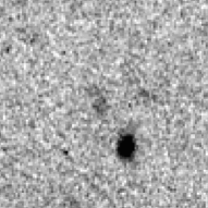
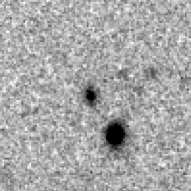
Figure 8: The figure shows the J-band image (left-hand panel) and the Ks-band image (right-hand panel) of source CDF-293. Both the images are 15$\times$15 arcsec centered on the source (RA=03:32:13, Dec=-27:46:41) This source is characterized by a color J-Ks=2.6 and an apparent magnitude Ks=20.4.

Figure 9: The J-band image (left-hand panel) and the Ks-band image (right-hand panel) of source HDFS-363 are shown. Both the images are 15$\times$15 arcsec centered on the source (RA=22:32:49, Dec=-60:32:11). This source is characterized by a color Js-Ks=3.3 and an apparent magnitude Ks=20.8.

In the CDF sample we count 7 sources (2$\%$ of the sample) redder than J-Ks=2.3 at Ks$\leq 22$, i.e. a surface density of about 1.2 per square arcmin. In the HDFS sample we selected 20 sources (5$\%$ of the sample) redder than Js-Ks=2.4 at Ks$\leq 22$, equivalent to a surface density of 2.7 per square arcmin. Six out of these 20 EROs lie out of the WFPC2 field and four on the borders. Four out of the remaining ten have no optical counterpart in the F814W band image.

The different surface densities found are most probably due to the clustering properties of EROs which introduce a strong field-to-field variation in small areas. Indeed, Daddi et al. (2000) detect a strong clustering signal of EROs selected on the basis of the R-K color from a K$\sim 19$ limited sample (see also McCarthy et al. 2000). They show that such clustering produces fluctuations on the surface densities of K$<19$ EROs 1.7 times higher than those expected from pure poissonian statistic on areas of the order of $\sim 25$ arcmin².

We selected EROs on a sample 3 magnitudes fainter and, in principle, on a different redshift range since we have used the J-Ks color selection. Thus, the results of Daddi et al. (2000) cannot be directly applied to our data. However, we could assume that the ERO clustering amplitude scales with K magnitude accordingly to the amplitude found for field K-band selected galaxies. On the basis of the results obtained by Roche et al. (1999) we thus expect that at Ks$\sim 21$ the ERO clustering is 1.25 times weaker than that derived by Daddi et al. at Ks$\sim$19. In the presence of a correlation with amplitude A, the fluctuations $\sigma$ of the counts around the mean value $\bar{n}$ are $\sigma=\sqrt{\bar{n}(1+\bar{n}AC)}$, being $C\propto Area^{-0.4}$. Applying this relation to our data, we derive an ERO surface density fluctuation $\sigma\sim 0.7$ which could be consistent with the fluctuations we observe.

In Fig. 8 and 9 the J and Ks-band images of the EROs CDF-293 and HDFS-363 are shown as an example. These sources have a J-Ks color of 2.6 and 3.3 respectively and an apparent Ks magnitude of 20.4 and 20.8. If they are elliptical galaxies at redshift $z\geq 2$, their k-corrected absolute magnitude would be $M_{Ks}<-25$, consistent with a passively evolved $M^{*}(z=0)$ galaxy.

Objects with extreme J-K color fainter than K$>20$ have been also found in the HDF-N by Dickinson et al. (2000) and in the HDF-S NICMOS field by Yahata et al. (2000). They discuss the possibility that they are dusty star-forming galaxies or ellipticals at $z>2$ or $z>10$ Lyman break galaxies. Maihara et al. (2000) notice that most of the red sources they found in the SDF appear as close neighbors, thus being probable interacting systems. We notice that $\sim 30\%$ of the red sources we found both in the CDF and in the HDFS are flagged as “blended” by SExtractor and that the remaining $70\%$ do not appear as close neighbors. A final possibility remains that some of the most compact sources at Ks$>21$ are faint very low-mass stars, which can display colors redder than J-K=2 (Chabrier et al. 2000; Dahn et al. 2000).

The analysis of the near-IR properties combined with those derived by photometry at optical wavelength will be presented in a forthcoming paper (Saracco et al. 2001).

6.3 Extremely blue sources

Figures 3 and 4 reveal the presence of objects with J-Ks color bluer than $\sim$0.8 mag, the color of a typical irregular galaxy. On the basis of the criteria we used to discriminate between star and galaxy (§3.2) those of them brighter than Ks$\sim$20 turned out to be stars. The remaining blue sources have been classified as galaxies since they have either a FWHM larger than a point source or a stellarity index lower than 0.9. However, almost all of them (14 in the CDF and 8 in the HDFS) are fainter than Ks=21 where star/galaxy classification is unfeasible in our data. Three out of the eight HDFS blue sources lie in the WFPC2 field: while two of them are pointlike in the F814W band image, the remaining one displays an irregular shape.

The first hypothesis we could make about the nature of these sources is that they are Galactic objects. In this case, a possible explanation for the blue IR color of at least some of them is that they are extreme M sub-dwarfs, similar to those studied by Leggett et al. (1998). These sources have metallicities as low as about one-hundredth solar, are characterized by effective temperatures T${}_{eff}\sim 3000$ K and by masses ranging 0.09-0.15 M_⊙. The objects analyzed by Leggett et al. have magnitudes in the range 9$<K<15$, colors J-Ks$\geq 0.4$ mag and absolute magnitudes in the range 9$<M_{K}<10$. Most of our extremely blue sources are in fact in this color range. Under the hypothesis that they are M sub-dwarfs with absolute magnitudes similar to those of Leggett et al., the present observations should have reached $\sim 6$ kpc considering a limiting magnitude Ks$\sim 22.5$.

Sources even bluer than J-Ks=0.4 and approaching J-K$\sim 0$ can be consistent with T-type brown dwarfs (e.g. Nakajima et al. 1995; Cuby et al. 1999). These IR extremely blue objects are characterized by red optical-IR colors. For instance, the methane brown dwarf NTTDF J1205-0744 (Cuby et al. 1999), the most distant reported to date, has a magnitude Ks=20.3. and colors J-K$\sim 0$, I-K$>6$. We reveal 3 faint sources in our samples with such a blue IR color: 2 in the CDF sample having J-Ks$\leq 0.3$ and 1 in the HDFS sample with J-Ks$\leq 0.1$. All of them are fainter than Ks=22 where the uncertainty in the color estimate is larger than 0.3 mag. If our three sources are methane brown dwarfs they have to be 2.5 times more distant than NTTDF J1205-0744 (considering $\Delta K=2$ magnitudes). The analysis of the optical data will help to assess the nature of these sources.

The second hypothesis about the nature of our extremely blue sources is that they are extragalactic objects. Using Bruzual & Charlot models we can account for colors less blue than 0.65, the case of a 1 Gyr old irregular galaxy at $z=0$ with a constant star formation (1 M_⊙/yr) and a metallicity lower than 0.2Z_⊙. Bluer colors can be obtained only assuming irregulars younger than 1Gyr. Another possibility is that these blue objects are $z>3$ sources with strong UV excess, like those reported by Sullivan et al. (2000). They debate the possibility that the UV light in these objects is due to a non-thermal source such as QSO/AGN perhaps superimposed on a star-forming component. In this case we would observe the rest-frame UV ($<3000$ Å) in the J band and wavelengths short-ward of $5500$ Å   in the Ks band. In fact, by red-shifting the mean energy distribution (MED) derived by Elvis et al. (1994) for quasars we are not able to produce colors bluer than 0.85 ($z\sim 3$). The large dispersion about this MED results in an uncertainty we estimate to be about $0.2-0.3$ mag. However, it is worth noting that QSOs showing colors as blue as J-K$\sim 0.6-0.5$ are observed also at redshift $z<3$ (Francis et al. 2000).

7 Summary and conclusions

We presented counts and colors of galaxies detected in the deep J and Ks images obtained with the near-IR camera ISAAC at the ESO VLT telescope centered on the Chandra Deep Field and on the Hubble Deep Field-South. The co-addition of short dithered 2.5$\times$2.5 arcmin images led to a total exposure time of about 8 hours in Ks and to a limiting surface brightness Ks$\simeq$22.8 mag/arcsec² and J$\simeq$24.5 mag/arcsec² on both the fields.

We found an excellent agreement between the counts derived in the two fields. On the other hand our counts and their slope lie in between those previously derived by other authors at comparable depth. In particular we estimate a slope of $\gamma_{J}$=0.34 and $\gamma_{K}$=0.28 at J$>20$ and Ks$>19$ respectively. We do not observe a turnoff in the counts down to the faintest magnitudes.

The observed J and Ks galaxy counts can be well fitted in a flat universe ($q_{0}=0.5$ or $\lambda_{0}>0$) only assuming models including some degree of merging. These models were previously found also to give a good fit to the optical number counts of the HDFS. On the contrary models not including merging are not able to reproduce the observed counts, independent of the cosmology.

Our estimated lower limits to the fraction of $z>1$ galaxies based on the J-K$>1.9$ color selection criterion are broadly consistent with the predictions for hierarchical models as well as for pure luminosity evolution models.

We identify 7 sources in the CDF (or 2$\%$ of the sample) and 20 source in the HDFS (or 5$\%$ of the sample) with colors redder than J-Ks=2.3 and magnitudes $20<Ks<22$, equivalent to a surface density of 1.2 and 2.7 sources per square arcmin respectively. Their extreme red colors suggest that they are old ellipticals or dusty star forming galaxies at redshift $z>2-3$. However some of the most compact of them could be very low-mass stars which can display very red near-IR colors. Another possibility, at least for the faintest and optically undetected ones, is that they are $z>10$ Lyman break galaxies.

A further analysis of their near-IR properties combined with those at optical wavelength will allow us to constraint their nature.

- (1) Arnouts S., D’Odorico S., Cristiani S., Zaggia S., Fontana A., Giallongo E., 1999, A&A 341, 641
- (2) Babul A., Rees M., 1992, MNRAS 255, 346
- (3) Balbi A., et al. 2000, astro-ph/0005124
- (4) Baugh C. M., Cole S., Frank C. S., 1996, MNRAS 283, 1361
- (5) Baugh, C. M.; Benson, A. J.; Cole, S.; Frenk, C. S.; Lacey, C. G., 1999, MNRAS 305, L21
- (6) Bernstein, G. M., Nichol, R. C., Tyson, J. A., Ulmer, M. P., Wittman, D. 1995, AJ, 110, 1507
- (7) Bershady, M. A., Lowenthal, J. D., Koo D. C. 1998, ApJ 505, 50
- (8) Bershady, M. A., Subbarao M., Koo D. C., Szalay A., Kron R. G., 1999, in preparation
- (9) Bertin, E., Arnouts, S., 1996, A&AS, 117, 393
- (10) Broadhurst T. J., Ellis R. S., Glazebrook K., 1992, Nat 355, 55
- (11) Bruzual A. G., Margis C. G., Calvert N., 1988, ApJ 333, 673
- (12) Bruzual A. G., Charlot S., 1993, ApJ 405, 538
- (13) Buzzoni A., 1989, ApJS 71, 817
- (14) Buzzoni A., 1995, ApJS 98, 69
- (15) Chabrier G., Baraffe I., Allard F., Haushildt P., 2000, ApJ 542, 464
- (16) Cowie, L. L., Gardner, J. P., Lilly S. J., McLean I., 1990, ApJ 360, L1
- (17) Cowie, L. L., Gardner, J. P., Hu, E. M., Songaila, A., Hodapp, K. W., Wainscoat, R. J. 1994, ApJ, 434, 114
- (18) Cuby J. G., Saracco P., Moorwood A. F. M., D’Odorico S., Lidman C., Comeron F., Spyromilio J., 1999, A&A 349, L41
- (19) Daddi E., Cimatti A., Pozzetti L., Hoekstra H., R ttgering H. J. A., Renzini A., Zamorani G., Mannucci F., 2000, A&A 361, 535
- (20) Dahn C. C., et al., 2000, in From Giant Planets to Cool Stars, ed. M. Marley and C. Griffith, in press
- (21) De Bernardis P. et al. 2000, astro-ph/0011469
- (22) De Propris, R., Eisenhardt, P. R., Stanford, S. A., Dickinson, M. 1998a, ApJ, 503
- (23) Dickinson M., Hanley C., Elston R., et al., 2000, ApJ 531, 624
- (24) Djorgovski, S., et al. 1995, ApJ, 438, L13
- (25) Eisenhardt P., Elston R., Stanford S. A., et al., 2000, (astro-ph/0002468)
- (26) Fontana A., Menci N., D’Odorico S., et al., 1999, MNRAS 310, L27
- (27) Fontana A., D’Odorico S., Poli F., et al., 2000, AJ 120, 2206
- (28) Francis P. J., Whiting M. T., Webster R. L. 2000, PASA 17, 56
- (29) Gardner, J. P., Cowie, L. L., Wainscoat, R. J. 1993, ApJ, 415, L9
- (30) Gardner, J. P., Sharples, M. R., Carrasco, B. E., Frenk, C. S., 1997, MNRAS 282, L1
- (31) Gardner, J. P., Sharples, M. R., Frenk, C. S., Carrasco, B. E. 1997, ApJ, 480, L99
- (32) Gardner, J. P., 1998, PASP 110, 291
- (33) Glazebrook, K., Peacock, J., Collins, C., Miller, L. 1994, MNRAS, 266, 65
- (34) Gronwall C., Koo D. C., 1995, ApJ 440, L1
- (35) Huang J.-S., Cowie L. L., Gardner J. P., Hu E. M., Songaila A., Wainscoat R. J. 1997, ApJ 476, 12
- (36) Kauffmann G., 1996, MNRAS 281, 487
- (37) Kauffmann G., Charlot S., 1998, MNRAS 297, L23
- (38) Le Fevre O., Abraham R., Lilly S. J., et al., 2000, MNRAS 311, 565
- (39) Leggett S. K., Allard F., Hauschildt P. H., 1998, ApJ 509, 836
- (40) Lobo, C., Biviano, A., Durret, F., Gerbal, D., Le Fevre, O., Mazure, A., Slezak, E. 1997, A&A, 317, 385
- (41) Maihara T., Iwamuro F., Tanabe H., et al., 2000, PASJ in press, (astro-ph/0009409)
- (42) Mamon G. A., 1998, in Wide field surveys in cosmology, XIV IAP Meeting, eds Colombi S., Mellier Y., Raban B., p. 323
- (43) Martini P., 2000, AJ submitted, (astro-ph/0008328)
- (44) Marzke, R. O., et al. 1994, AJ, 108, 436
- (45) Marzke, R. O., Da Costa, L. N. 1997, AJ, 113, 1
- (46) McCarthy P., Carlberg R., Marzke R., et al. 2000, (astro-ph/0011499)
- (47) McCracken H. J., Metcalfe N., Shanks T., Campos A., Gardner J. P., Fong R., 2000, MNRAS 311, 707
- (48) McLeod, B. A., Bernstein, G. M., Reike, M. J., Tollestrup, E. V., Fazio, G. G., 1995, ApJS, 96, 117
- (49) Metcalfe N., Shanks T., Campos A., McCracken H. J., Fong R., 2000, MNRAS in press (astro-ph/0010153)
- (50) Minezaki, T., Kobayashi, Y., Yoshii, Y., Peterson, B. A., 1998, ApJ, 494, 111
- (51) Molinari E., Chincarini G., Moretti A., De Grandi S., 1998, A&A 338, 874
- (52) Moorwood A. F. M. , Cuby J. G., Ballester P., et al., 1999, The Messenger 95, 1
- (53) Moustakas, L. A., Davis, M., Graham, J. R., Silk, J., Peterson, B. A., Yoshii, Y., 1997, ApJ, 475, 445
- (54) Nakajima T., Oppenheimer B. R., Kulkarni S. R., Golimowski D. A., Matthews K., Durrance S. T. 1995, Nature 378, 463
- (55) Peacock J. A., 1987, in em Astrophysical Jets and their Engines, ed. Kundt W., 171, Reidel Dordrecht
- (56) Perlmutter S., et al., 1999, ApJ 517, 565
- (57) Persson E., Murphy D. C., Krzeminski W., Roth M., Rieke M. J., 1998, AJ 166, 2475
- (58) Pozzetti L., Bruzual A. G., Zamorani G., 1996, MNRAS 281, 953
- (59) Pozzetti L., Madau P., Zamorani G., Ferguson H., Bruzual A. G., 1998, MNRAS 298, 1133
- (60) Riess A. G., et al., 1998, AJ 116, 1009
- (61) Roche N., Eales S. A., Hippelein H., Willot C. J., 1999, MNRAS 306, 358
- (62) Rocca-Volmerange B., Guiderdoni B., 1990, MNRAS 247, 166
- (63) Saracco P., Iovino, A., Garilli, B., Maccagni, D., Chincarini, G., 1997, AJ, 114, 887
- (64) Saracco P., D’Odorico S., Moorwood A. F. M., Buzzoni A., Cuby J. G., Lidman C., 1999, A&A 349, 751
- (65) Saracco P., et al., 2001, in preparation
- (66) Sullivan M., Treyer M. A., Ellis R. S., Bridges T. J., Milliard B., Donas J., 2000, MNRAS 312, 442
- (67) Szokoly, G. P., Subbarao, M. U., Connolly, A. J., Mobasher, B. 1998, ApJ, 492, 452
- (68) Teplitz H. I., Gardner J. P., Malumuth E. M., Heap S. R., 1998, ApJ 507, L17
- (69) Vaisanen P., Tollestrup E. V., Willner S. P., Cohen M., 2000, ApJ in press (astro-ph/0004224)
- (70) Vanzella E., Cristiani S., Saracco P., Arnouts S., Fontana A., Giallongo E., Grazian A., Iovino A., 2001, AJ, in preparation
- (71) Volonteri M., Saracco P., Chincarini G., Bolzonella M., A&A 362, 487
- (72) Wang B., 1991, ApJ 383, L37
- (73) Yahata N., Lanzetta K. M., Chen H-W., et al. 2000, ApJ 538, 493
- (74) Zucca, E., et al. 1997, A&A, 326, 477