WeCAPP - The Wendelstein Calar Alto Pixellensing Project I

Abstract

We present WeCAPP, a long term monitoring project searching for microlensing events towards M 31. Since 1997 the bulge of M 31 was monitored in two different wavebands with the Wendelstein 0.8 m telescope. In 1999 we extended our observations to the Calar Alto 1.23 m telescope. Observing simultaneously at these two sites we obtained a time coverage of 53 % during the observability of M 31. To check thousands of frames for variability of unresolved sources, we used the optimal image subtraction method (OIS) by Alard & Lupton (1998). This enabled us to minimize the residuals in the difference image analysis (DIA) and to detect variable sources with amplitudes at the photon noise level. Thus we can detect microlensing events with corresponding amplifications $A>10$ of red clump giants with $M_{\mathrm{I}}=0$.

1 Introduction

In the last decade microlensing studies proved to be a powerful tool for searching baryonic dark matter in the Galactic halo.
Several groups like the MACHO collaboration (Alcock et al., 1993), OGLE (Udalski et al., 1993), EROS (Aubourg et al., 1993) and DUO (Alard et al., 1995) followed the suggestion of Paczynski (1986) and surveyed millions of stars in the Large and Small Magellanic Clouds (LMC, SMC) and in the Galactic bulge for variability induced by gravitational microlensing. Although all of them discovered events compatible with gravitational lensing by MACHOs (Massive Astrophysical Compact Halo Objects) (Paczynski et al., 1994; Ansari et al., 1996; Alcock et al., 1997; Alard & Guibert, 1997; Palanque-Delabrouille et al., 1998; Alard, 1999; Afonso et al., 1999; Alcock et al., 2000a, b; Udalski et al., 2000) they were not able to derive unambiguous constraints on the amount of baryonic dark matter and its distribution in the Galactic halo (e.g. Lasserre et al., 2000; Evans & Kerins, 2000, and references therein).
Crotts (1992) and Baillon et al. (1993) suggested to include M 31 in future lensing surveys and pointed out that it should be an ideal target for these kind of experiments. In contrast to microlensing studies towards the LMC and the SMC, which are restricted to similar lines of sight through the Galactic halo, one can study many different lines of sight to M 31, which allow to separate between self-lensing and true MACHO events.
Since the optical depth for Galactic MACHOs is much greater towards M 31 than towards the LMC, SMC or the Galactic bulge one expects event rates greater than in previous lensing studies. Furthermore M 31 contributes an additional MACHO population as it possesses a dark halo of its own. Thus, three populations may contribute to the optical depth along the line of sight: MACHOs in the Galactic halo, MACHOs in the halo of M 31 and finally stars in the bulge and the disk of M 31 itself, a contribution dubbed self-lensing.
The high inclination of M 31 ($77^{\circ}$) (Walterbos & Kennicutt, 1987) produces a near-far asymmetry of the event rates. The near side of the M 31 disk will show less events than the more distant one (Crotts, 1992). Since Galactic halo-lensing as well as self-lensing events will not show this feature, a detected asymmetry will be an unambiguous proof for the existence of M 31 MACHOs.
As most of the sources for possible lensing events are not resolved at M 31’s distance of 770 kpc (Freedman & Madore, 1990) the name ‘pixellensing’ (Gould, 1996) was adopted for these kind of microlensing studies. In the mid nineties two projects started pixellensing surveys towards M 31, AGAPE (Ansari et al., 1997) and Columbia/VATT (Tomaney & Crotts, 1996). First candidate events were reported (Ansari et al., 1999; Crotts & Tomaney, 1996) but could not yet be confirmed as MACHOs. This was partly due to an insufficient time coverage which did not rule out variable stars as possible sources.
1999 two new pixellensing projects, POINT-AGAPE (Kerins & the Point-Agape Collaboration, 2000), who reported recently a first candidate microlensing event (Auriere et al., 2001), and MEGA (Crotts et al., 1999), the successor of Columbia/VATT, began their systematical observations of M 31. Another project, SLOTT-AGAPE (Slott-Agape Collaboration, 1999) will join them this year.
The Wendelstein Calar Alto Pixellensing Project started with a test and preparation phase on Wendelstein as WePP in autumn 1997 before it graduated after two campaigns to WeCAPP in summer 1999 by using two sites for the survey.
In this paper we will give an introduction to the project including information about the data obtained in three years and our reduction pipeline. In Sect. 2 we briefly discuss the basic principles of pixellensing. In Sect. 3 we will give an overview of the project including information about the sites used and the data obtained during WeCAPP. Section 4 refers to our data reduction pipeline and describes how light curves are extracted. In Sect. 5 we show first light curves and Sect. 6 summarizes the paper.

2 Pixellensing

In microlensing surveys of uncrowded fields a resolved star is amplified by a function $A$ which can be measured from the light curve and which yields direct information of the lensing parameters (Paczynski, 1986):

$$A(u)=\frac{u^{2}+2}{u\sqrt{u^{2}+4}}\;;\;u^{2}=\mu_{\mathrm{E}}^{2}(t-t_{0})^{2}+u_{0}^{2}$$ (1)

with $\mu_{\mathrm{E}}=1/t_{\mathrm{E}}$, the inverse Einstein ring crossing time, $u_{0}$ the angular impact parameter in units of the angular Einstein ring radius $\theta_{\mathrm{E}}$ and $t_{0}$ the time of maximum amplification.
The angular Einstein ring radius $\theta_{\mathrm{E}}$ is connected with the physical Einstein ring radius $r_{\mathrm{E}}$ and the properties of the gravitational lens by

$$\theta_{\mathrm{E}}=\frac{r_{\mathrm{E}}}{D_{\mathrm{l}}}\;;\;r_{\mathrm{E}}=\bigg{(}\frac{4GM}{c^{2}}\frac{D_{\mathrm{l}}D_{\mathrm{ls}}}{D_{\mathrm{s}}}\bigg{)}^{\frac{1}{2}}$$ (2)

with the mass of the lens $M$, and the distances between the observer and lens $D_{\mathrm{l}}$, observer and source $D_{\mathrm{s}}$, and lens and source $D_{\mathrm{ls}}$. According to Eq. 1 a lensing event will produce a symmetric and, as lensing does not depend on the colour of the source, achromatic light curve (see also Sect. 3).
In more crowded fields it is not possible to determine the amplification $A$ unambiguously because many unresolved sources may lie inside the solid angle of the point spread function $\Omega_{\mathrm{PSF}}$ of a bright source. If one of these unresolved sources is amplified, the event could erroneously be attributed to the bright star, which results in a strong amplification bias (Han, 1997; Alard, 1997; Wozniak & Paczynski, 1997; Goldberg, 1998).
Similarly, in pixellensing studies the true amplification cannot be determined because many stars fall in one resolution element.
Nevertheless one can still construct a light curve $\Delta F(t)$ by subtracting a reference frame from the image, in which a lensing event takes place:

$$\Delta F(t)=F(t)-B=F_{i}\cdot[A(t)-1]\;;\;B=F_{i}+B_{\mathrm{res}}$$ (3)

with $F_{i}$ the flux of the source after or before lensing and $B_{\mathrm{res}}=\sum_{j\neq i}F_{j}$ being the residual flux from unlensed sources inside $\Omega_{\mathrm{PSF}}$. As there are many sources contributing to the flux inside $\Omega_{\mathrm{PSF}}$, pixellensing events will only be detected if the amplification $A$ or the intrinsic flux $F_{i}$ of the lensed source are high. However, this difficulty in identifying events is balanced by the large number of possible sources for lensing events in the bulge of M 31.
As pointed out by Gould (1996), the main difference between classical microlensing and pixellensing consists in the fact, that in the latter case the noise within $\Omega_{\mathrm{PSF}}$ is dominated by unlensed sources and therefore stays virtually constant during an event. As only events with a high amplification can be detected, the Einstein timescale $t_{\mathrm{E}}$ is not a general observable in pixellensing. Therefore $t_{\mathrm{FWHM}}$ which describes the width of a lensing light curve at half of its maximum value is the only timescale one is able to measure with a certain accuracy. Based on a previous work of Gondolo (1999), who pointed out that the optical depth towards M 31 can be estimated without knowing $t_{\mathrm{E}}$, Baltz & Silk (2000) showed how the measurement of a moment of the light curve $t_{\sigma n}$ permits to calculate the Einstein time $t_{\mathrm{E}}$ for a particular lensing event. Furthermore principal component analysis of the light curves can yield a less biased information about the mass function of the lenses as shown by Alard (2001).
Han (1996) has estimated the amount of expected microlensing events with a cumulative event signal-to-noise ratio $(S/N)_{\mathrm{min}}=20$ (for a further description see Gould, 1996). The assumption he used was that the whole dark matter halo consists of MACHOs. The calculations are mainly depending on the luminosity function of the M 31 stars and on the spatial distribution of the lenses. From Han’s paper we derive the following scaling relation for the event rate:

$$\Gamma = 94\,\mathrm{ev/yr}\;{\left(\frac{t_{\mathrm{camp}}}{1/3\,\mathrm{yr}}\right)}{\left(\frac{t_{\mathrm{cyc}}}{1\,\mathrm{d}}\right)}^{-1}{\left(\frac{t_{\mathrm{exp}}}{4\,\mathrm{h}}\right)}{\left(\frac{\epsilon}{12\,\mathrm{phot/s}}\right)}\cdot$$ (4)

$$\cdot{\left(\frac{\theta_{\mathrm{see}}}{1\,\arcsec}\right)}^{-2}{\left(\frac{\eta_{\mathrm{sky}}^{2}+\eta_{\mathrm{psf}}^{2}}{3.35}\right)}^{-1}{\left(\frac{\Omega_{\mathrm{ccd}}}{70\,\mathrm{arcmin}^{2}}\right)}$$

For the typical parameters of our 1999/2000 campaign this results in a predicted event rate $\Gamma=27\,\mathrm{ev/yr}$, with the length of the campaign $t_{\mathrm{camp}}=260\,\mathrm{d}$, the average time span between observations $t_{\mathrm{cyc}}=2\,\mathrm{d}$, the exposure time per night $t_{\mathrm{exp}}=0.5\,\mathrm{h}$, the photon detection rate $\epsilon=43\,\mathrm{phot/s}$, the median seeing $\theta_{\mathrm{see}}=1.5\,\mathrm{arcsec}$, the area of the image $\Omega_{\mathrm{ccd}}=70\,\mathrm{arcmin}^{2}$, the inaccuracy of the PSF matching $\eta_{\mathrm{psf}}^{2}=0$, and the factor in the noise due to sky photons $\eta_{\mathrm{sky}}^{2}=2.6$.
This calculation can only serve as a crude estimate of the event rate. In our subsequent papers we will present calculations more appropriate for our data set.

3 The WeCAPP Project

3.1 Telescopes and Instruments

The Wendelstein 0.8 m telescope has a focal length $f$ of 9.9 m, which results in an aperture ratio $f/D=12.4$. Starting in September 1997 we used a TEK CCD with $1024\times 1024$ pixels of $24\,\mu\mathrm{m}$ corresponding to 0.5 arcsec on the sky. With this CCD chip we were able to cover $8.3\times 8.3\,\mathrm{arcmin}^{2}$ of the bulge of M 31. To increase the time sampling of our observations we started to use the Calar Alto 1.23 m telescope ($f=9.8\,\mathrm{m}$, $f/D=8.0$) in 1999. The observations were partly carried out in service mode. Six different CCD chips were used. Three of these CCDs cover a field of $17.2\times 17.2\,\mathrm{arcmin}^{2}$ and were used to survey the whole bulge for lensing events. A detailed overview of the properties of each CCD camera used for WeCAPP is given in Table 1.

Site	Campaign	CCD	Size	[$\mathrm{arcsec}/\mathrm{px}$]	Field [$\mathrm{arcmin}^{2}$]	# of R frames	# of I frames
We	1997/1998	TEK#1	1K $\times$ 1K	0.49	$8.3\times 8.3$	276	123
We	1998/1999	TEK#1	1K $\times$ 1K	0.49	$8.3\times 8.3$	454	210
We	1999/2000	TEK#1	1K $\times$ 1K	0.49	$8.3\times 8.3$	835	358
CA	1999/2000	TEK7c_12	1K $\times$ 1K	0.50	$8.6\times 8.6$	266	136
CA	1999/2000	TEK13c_15	1K $\times$ 1K	0.50	$8.6\times 8.6$	62	33
CA	1999/2000	SITe2b_11	2K $\times$ 2K	0.50	$17.2\times 17.2$	14	7
CA	1999/2000	SITe2b_17	2K $\times$ 2K	0.50	$17.2\times 17.2$	448	249
CA	1999/2000	SITe18b_11	2K $\times$ 2K	0.50	$17.2\times 17.2$	165	91
CA	1999/2000	LOR11i_12	2K $\times$ 2K	0.31	$10.75\times 10.75$	219	92

Table 1: Properties of all CCD cameras used during WeCAPP at Wendelstein (We) and Calar Alto (CA) Observatories, respectively. All CCDs have a pixel size of $24\,\mu\mathrm{m}$, except the Loral which has $15\,\mu\mathrm{m}$ pixels.

Most of the sources for possible lensing events in the bulge of M 31 are luminous red stars i.e. giants and supergiants. Consequently the filters used in our project should be sensitive especially to these kind of stars. We chose therefore R and I filters for our survey. At Wendelstein we used the R2 ($\lambda\simeq 650\,\mathrm{nm}$, $\Delta\lambda\simeq 150\,\mathrm{nm}$) and Johnson I ($\lambda\simeq 850\,\mathrm{nm}$, $\Delta\lambda\simeq 150\,\mathrm{nm}$) wavebands. To be as consistent as possible with the data obtained at Wendelstein, the Calar Alto observations were carried out with the equivalents filters, R2 ($\lambda\simeq 640\,\mathrm{nm}$, $\Delta\lambda\simeq 150\,\mathrm{nm}$) and Johnson I ($\lambda\simeq 850\,\mathrm{nm}$, $\Delta\lambda\simeq 150\,\mathrm{nm}$). Since June 2000 we are using the newly installed filters Johnson R ($\lambda\simeq 640\,\mathrm{nm}$, $\Delta\lambda\simeq 160\,\mathrm{nm}$) and Johnson I ($\lambda\simeq 850\,\mathrm{nm}$, $\Delta\lambda\simeq 150\,\mathrm{nm}$) at Calar Alto.
Despite of the combination of different telescopes, CCDs, and slightly different filter systems we observed no systematic effects in the light curves depending on these parameters.

3.2 Observing Strategy

To follow the suggestion of Tomaney & Crotts (1996) and Han & Gould (1996) we chose the field with the maximal lensing probability, pointing to the far side of the M 31 disk. The main fraction of the field is covered by the bulge of M 31 with the nucleus of M 31 located at one corner of the field (Fig. 1).

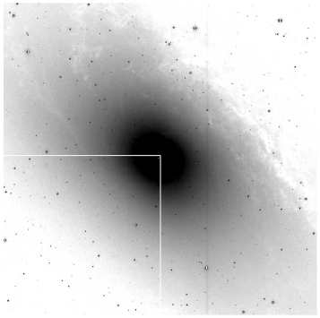
Figure 1: M 31 frame observed on 2000 June 26th with the Calar Alto 1.23 m telescope: $17.2\times 17.2\;\mathrm{arcmin}^{2}$ ($3.85\times 3.85\;\mathrm{kpc}^{2}$). A quarter of this field, marked by the solid lines, was observed during the first three campaigns from September 1997 until March 2000.

As gravitational lensing is achromatic, the amplification of the source is the same in different wavebands. However, as shown in several papers (e.g. Valls-Gabaud, 1994; Witt, 1995; Han et al., 2000) blending on the one hand and differential amplification of an extended source on the other hand can lead to a chromatic, but still symmetric, lensing light curve. Under certain circumstances chromatic light curves permit to constrain the physical properties of the source-lens system (e.g. Gould & Welch, 1996; Han & Park, 2001). Variable stars will generally change colour in a different way. Our observation cycle therefore comprises 5 images in the R band and 3 images in the I band lasting about 45 min including readout time. Stacking these images with an average exposure time of 150 sec in R and 200 sec in I results in a magnitude limit between (20.8 – 22.1) mag in R and (19.1 – 20.4) mag in I for a point source on the background of M 31 and a signal-to-noise ratio $(S/N)=10$ in over 95 % of the frame. The background of M 31 typically has a surface brightness between (18.7 – 21.2) $\mathrm{mag}/\mathrm{arcsec}^{2}$ in R and (16.8 – 19.3) $\mathrm{mag}/\mathrm{arcsec}^{2}$ in I. The cycles were repeated as often as possible during one night, usually at least twice. As we had to avoid saturation of stars in the observed field we made exposure times dependent of the actual seeing, whereas exposure times in the I bands where generally longer.

3.3 The Data

We began our observations at Wendelstein with a test period in September 1997, observing on 35 nights until March 1998. The second observational period lasted from 1998 October 22nd until 1999 March 24th . During the first Calar Alto campaign we received two hours of service observations on 87 of 196 allocated nights (1999 June 27th - 2000 March 3rd). From November 1st until November 14th we were able to observe during the whole night. In parallel we continued our observations at Wendelstein on 221 nights, of which 65 were clear. In this way we achieved an overall time coverage of 132 nights (52.6 %). During the three years of WeCAPP we collected at Wendelstein Observatory a total of 1565 images in the R band and 691 images in the I band. The observations for over more than one year at Calar Alto resulted in 1174 frames in the R and 608 frames in the I band.
During the 1997/1998 test campaign conditions at the Wendelstein telescope were improved significantly. A newly installed air conditioning system reduced dome seeing to a low level. Further improvements like fans just above the main mirror finally lead to a leap in the image quality obtained with the telescope. Figure 2 which presents the PSF statistics of Wendelstein images from the 1997/1998 and 1998/1999 campaigns respectively illustrates this fact. In general Wendelstein shows a marginally better PSF distribution than Calar Alto (see Figs. 2 and 3). Table 2 shows the PSF median values for the images taken during WeCAPP at both sites.

Filter	We 1997/1998	We 1998/1999	We 1999/2000	CA 1999/2000
R	2.76	1.45	1.40	1.49
I	2.59	1.44	1.32	1.44

Table 2: Median values of the FWHM of the PSF, given in arcsec, for the images taken during WeCAPP in the R and I band at Wendelstein and Calar Alto Observatories.

Figure 2: Histograms of the Full Width Half Maximum (FWHM) of the point spread function (PSF) of the frames taken at Wendelstein Observatory during the 1997/1998 campaign (left panel) and the 1998/1999 campaign (right panel). Frames in the R band are marked by a solid line, frames in the I band by a dashed line. The lower limit of the PSF is restricted by a pixel size of 0.5 arcsec.

Figure 3: Histograms of the FWHM of the frames taken during the 1999/2000 campaign at Wendelstein (left panel) and Calar Alto Observatory (right panel). Frames in the R band are marked by a solid line, frames in the I band by a dashed line. Note that the pixel sizes of the CCD cameras used correspond to 0.5 arcsec on the sky.

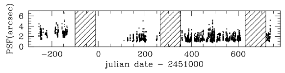
Figure 4: Illustration of PSF vs. time coverage during three years of WeCAPP. Shaded regions mark the periods of time when M 31 was not observable.

Figure 4 shows the time sampling we reached so far with WeCAPP. Because of time loss during the upgrades of the telescope, time coverage of the 1997/1998 campaign is only fragmentary. About the same applies to the following campaign, this time due to a camera shutdown and another time consuming project. Finally time coverage of the first joint campaign of Wendelstein and Calar Alto is good, last but not least due to the often opposite weather situation in Spain and Germany.

4 Data Reduction

4.1 Reduction Pipeline

In the last three years we developed an image reduction pipeline being able to cope with a massive imaging campaign. This reduction pipeline is described in detail in Gössl & Riffeser (2001) and combines all reduction steps from de-biasing of the images until the final measurements of the light curves in one software package, including full error propagation from the first reduction step to the last:

1. standard CCD reduction including de-biasing, flat-fielding and filtering of cosmics

2. position alignment using a 16 parameter interpolation

3. stacking of frames

4. photometric alignment

5. PSF matching using OIS (Optimal Image Subtraction), a method proposed by Alard & Lupton (1998)

6. generation of difference images

7. detection of variable sources

8. photometry of the variable sources

4.2 Standard CCD Reduction

Pre-reduction of the raw frames is performed in a standard way: After de-biasing of the frames, saturated and bad pixels are marked. We use the 3 $\sigma$ clipped median of a stack of at least 5 twilight flatfields for the flat fielding procedure.
Cosmics are effectively detected by fitting a Gaussian PSF to all local maxima in the frame. All PSFs with a FWHM lower than 0.7 arcsec and an amplitude of 8 times the background noise are removed. This provides a very reliable identification and cleaning of cosmics.

4.3 Position Alignment

After determining the coordinates of the reference objects by a PSF fit, we calculate a linear coordinate transformation to project an image onto the position of the reference frame.
The flux interpolation for non-integer coordinate shifts is calculated from a 16-parameter, $3^{\mathrm{rd}}$-order polynomial interpolation using 16 pixel base points.

4.4 Stacking Frames

To avoid saturation of Galactic foreground stars and the nucleus of M 31 in our field, exposure times were limited to a few hundred seconds. Therefore one has to add several frames taken in one cycle to obtain an acceptable signal-to-noise ratio $(S/N)$. Usually we stacked 5 frames in the R band and 3 frames in the I according to two criteria, comparable PSF and comparable sky. Frames with very high background levels or very broad PSFs were not added if they reduced the detectability of faint variable sources. Consequently the number of images to be stacked was not fixed, coaddition of frames was performed in a way to get a maximum $(S/N)$ ratio for faint point sources in the stacked frame.
Before OIS is finally carried out we align all frames photometrically. This ensures that all light curves are photometrically calibrated to a standard flux.

4.5 PSF Matching

In order to extract light curves of variable sources from the data we use a method called Difference Image Analysis (DIA), proposed by Ciardullo et al. (1990) and first implemented by Tomaney & Crotts (1996) in a lensing study.
The idea of DIA is to subtract two positionally and photometrically aligned frames which are identical except for variable sources. The resulting difference image should than be a flat noise frame, in which only the variable point sources are visible.
The crucial point of this technique apart from position registration is the requirement of a perfect matching of the point spread functions (PSFs) between the two frames.
The PSF of the reference frame $r$ is convolved with a kernel $k$ to match the broader PSF of an image $i$,

$$i(x,y)\approx r(u,v)\otimes k(u,v)+bg(x,y)\equiv\tilde{r}(x,y)$$ (5)

where $bg$ accounts for the background level and $\tilde{r}$ is the transformed reference frame.
In order to obtain an optimal kernel $k$ we implemented OIS as proposed by Alard & Lupton (1998). This least-squares fitting method determines $k$ by decomposing it into a set of basis functions. We use a combination of three Gaussians with different widths $\sigma$ multiplied with polynomials up to $6^{\mathrm{th}}$ order. This leads to the following $49$ parameter decomposition of $k(u,v)$:

$$\begin{array}[]{rl}\sigma_{1}=1:&e^{-\frac{u^{2}+v^{2}}{2\sigma_{1}^{2}}}\;(a_{1}+\dots+a_{22}u^{6}+\dots+a_{28}v^{6})\\ \sigma_{2}=3:&e^{-\frac{u^{2}+v^{2}}{2\sigma_{2}^{2}}}\;(a_{29}+...+a_{39}u^{4}+...+a_{43}v^{4})\\ \sigma_{3}=9:&e^{-\frac{u^{2}+v^{2}}{2\sigma_{3}^{2}}}\;(a_{44}+\dots+a_{47}u^{2}+a_{48}uv+a_{49}v^{2})\end{array}$$ (6)

Additionally 3 parameters are used to fit the background

$$bg(x,y)=a_{50}+a_{51}\,x+a_{52}\,y\;.$$ (7)

To cope with the problem of a PSF varying over the area of the CCD we divide the images in sub-areas of 141 x 141 pixels each. In all sub-areas a locally valid convolution kernel is calculated. As we have chosen the kernel to have 21 x 21 pixels we therefore effectivly use 161 x 161 to derive $k(u,v)$.
Differential refraction causes a star’s PSF to depend on its colour (Tomaney & Crotts, 1996, chap. 4.4). However these second order effects are negligible for our data set and do not lead to residuals in the difference images.
As we are performing DIA we have to choose a reference frame $r$ which will be subtracted from all other coadded frames $i$ and which determines the baseline of the light curve. OIS shows best results for a small PSF and a high $(S/N)$ reference frame. Therefore, the best stacked images were coadded once more. Our actual R band reference frame comprises 20 images taken at 2 different nights resulting in a total exposure time of 2400 seconds and a PSF of a FWHM of 1.05 arsec (= 2 pixels for all CCDs except one at Wendelstein and Calar Alto). For the I band we coadded 18 frames (i.e. 6 stacked frames taken at 3 different nights) which results in a total exposure time of 3160 seconds and a FWHM of 1.15 arcsec. As we are continuing collecting data the process of constructing the ultimate reference frame has not finished yet. Each night of high quality data collected at one of the two sites will improve the reference frame further. Figure 5 shows a typical difference image obtained by using our implementation of OIS.

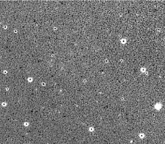
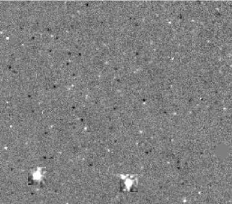
Figure 5: Difference images of a part of the M 31 bulge ($3.25\times 2.82\,\mathrm{arcmin}^{2}$), centered at 6.6 arcmin distance from the nucleus. Left panel: difference frame without OIS. Because of the relatively large residuals from stars no identification of faint variable stars is possible. Right panel: difference frame with OIS. Bright and dark spots are variable sources. The two boxes represent stars not subtracted in order to provide information on the PSF.

4.6 Source Detection

To detect sources in the difference images we fit a rotated Moffat function (Moffat, 1969) to all local maxima in the binned frame. Real sources are filtered by rejecting sources with an amplitude less than 5 times the background noise.

4.7 Photometry of the variable sources

Photometry of the detected sources is performed by a profile fitting technique. To obtain information about the PSF of any particular frame we apply a Moffat fit (Moffat, 1969) to several reference stars in the CCD field. Having determined the shape of the PSF, we perform Moffat fits on the positions of the variable sources as returned from the detection algorithm. In these final fits the amplitude is the only free parameter. To determine the flux of the source we finally integrate the count rates over the area of the (now fully known) analytical function of the PSF. This minimizes the contamination from neighbouring sources.

4.8 Calibration of the Light Curves

As the coadded images are normalized to the reference frame it is not necessary to calibrate each image separately. Only the reference frame is calibrated once.
To calculate magnitudes $m_{\mathrm{R^{\prime}}}$ in our $\mathrm{R^{\prime}}$ band, which corresponds to R2, we determined the instrumental zeropoint $ZP_{\mathrm{R^{\prime}}}$ and the extinction coefficient $\kappa$:

$$m_{\mathrm{R^{\prime}}}=-2.5\log[ADU/t]-\kappa\cdot AM+ZP_{\mathrm{R^{\prime}}}$$ (8)

where $t$ is the exposure time and $AM$ is the airmass.
Aperture photometry with 7 different Landolt standard stars (Landolt, 1992) observed at different airmasses was performed for a photometric night at Calar Alto Observatory. With these stars the extinction $\kappa$ for the night was calculated to $\kappa_{\mathrm{R^{\prime}}}=0.073\pm 0.005$. To determine the zeropoint for the $\mathrm{R^{\prime}}$ band we used an A0V-star, Feige 16, with the colours $(B-V)=-0.012$, $(U-B)=0.009$, $(V-R)=-0.003$, $(R-I)=0.002$, and a visual magnitude of $V=12.406$ mag. The zeropoint was determined according to Eq. 8 to $ZP_{\mathrm{R^{\prime}}}=23.05\pm 0.02\ \mathrm{mag}$ and used to calculate the magnitudes for the reference frame. This zeropoint is not valid for Wendelstein.
In the following, we only give fluxes for the sources in our filter system, because the intrinsic magnitudes and colours of our unresolved sources cannot be determined with sufficient accuracy.
We show the light curves in flux differences according to

$$\Delta f_{\mathrm{R^{\prime}}}=f_{\mathrm{R^{\prime},Vega}}\frac{\Delta ADU_{\mathrm{R^{\prime}}}}{t}10^{0.4\,\kappa\ \mathrm{AM}}10^{-0.4\,ZP_{\mathrm{R^{\prime}}}}$$ (9)

with $f_{\mathrm{R^{\prime},Vega}}=3124\,\mathrm{Jy}$ from an integration over the CCD-filter system.
The same transformations were done for our $\mathrm{I^{\prime}}$ band, corresponding to Johnson I (Calar Alto), with $\kappa_{\mathrm{I^{\prime}}}=0.025\pm 0.005$, $ZP_{\mathrm{I^{\prime}}}=21.82\pm 0.03\,\mathrm{mag}$ and $f_{\mathrm{I^{\prime},Vega}}=2299\,\mathrm{Jy}$.
The colour terms between all filter sets we used in our observation are negligible. The transformation to the standard Kron-Cousins filter system is: $R=R^{\prime}+ZP_{\mathrm{R^{\prime}}}+0.06(R-I)$, $I=I^{\prime}+ZP_{\mathrm{I^{\prime}}}+0.38(R-I)$.

5 Results

We present a small sample of light curves to show the efficiency of the method. All light curves were observed over more than three years from 1997 until 2000. Time spans when M 31 was not observable are marked by shaded regions. Because of bad dome seeing conditions and an inappropriate autoguiding system errors were largest during the first Wendelstein campaign 1997/98. During the second period 1998/99 we were able to decrease the FWHM of the PSF by a factor of two, thus the photometric scatter is also clearly smaller. During the third period 1999/2000 we observed simultaneously at Calar Alto and Wendelstein and got data points for 53 % of the visibility of M 31.
The OIS method can be applied for very crowded fields like M 31 and gives residual errors at the photon noise level (Fig. 6), see also Gössl & Riffeser (2001)).

Figure 6: Histogram of the pixel values of a simulated difference image $d_{xy}=i_{xy}-r_{uv}\otimes k_{uv}$ ($r$ is the reference frame, $i$ is a second frame and $k$ is the convolution kernel). The pixel values are divided by the expected rms errors, as derived from error propagation. The solid curve shows a Gaussian with $\sigma=1$. We calculated the reduced chi-square $\chi^{2}_{\mathrm{dof}}$ of 19 different simulated images in the range between -3 and 3. The median $\bar{\chi}^{2}_{\mathrm{dof}}$ is 1.1, which means that expected and measured errors match almost perfectly and that the residuals of the OIS are at the photon noise level.

A good estimate for the average noise present in the area $\Omega_{\mathrm{PSF}}$ of a PSF is $N=0.1\times 10^{-5}\mathrm{Jy}$. The light curves of variable stars presented in the Figs. 7 through 16 indicate a typical scatter which is in good agreement with the above estimate. This means that a red clump giant with a brightness of $M_{\mathrm{I}}=0$ (Grillmair et al., 1996, Fig. 7) and a colour of $(R-I)=0.5$ (Lejeune et al., 1998) has to be amplified by a factor of 10 to be detected with a peak signal-to-noise ratio of $(S/N)=3$ in our survey. The brightest RGB stars with a $M_{\mathrm{I}}=-3.5$ and a colour of $(R-I)=1$ need an amplification of 1.6 only.
Up to now we detected over 5000 variable sources in a $8\times 8\,\mathrm{arcmin}^{2}$ field. A preliminary analysis of the light curves shows that we have found the whole range of variable stars including novae and other types of eruptive variables, Cepheids, semi-regular, Mira-type and other longperiodic variables.
In Fig. 7 we present one of the $\delta$-Cephei variable stars in the $\mathrm{R^{\prime}}$ and $\mathrm{I^{\prime}}$ bands, Fig. 8 shows the $\mathrm{R^{\prime}}$ light curve of this star convolved with its period, which was determined to $15.76\pm 0.01$ days. Figure 9 presents the light curve of a nova previously published by Modjaz & Li (1999). It’s the brightest variable source detected in our M 31-field. Figure 10 is an example for an eruptive variable star, which could be mistaken as a microlensing event, if the time coverage were insufficient. Figures 11 to 15 display light curves of variable stars, which were classified as longperiodic in a preliminary analysis. Finally we present the light curve of a RV Tauri star in Fig. 16.

Figure 7: Light curve of a $\delta$-Cephei variable, upper panel: $\mathrm{R^{\prime}}$ band, lower panel: $\mathrm{I^{\prime}}$ band.

Figure 8: Light curve of the $\delta$-Cephei star of Fig. 7 in the $\mathrm{R^{\prime}}$ band, convolved with its period of $P=15.76\pm 0.01$ d. Plotted without (left panel) and with (centre panel) $1\sigma$ error bars, which represent fully propagated errors through all reduction steps. Right panel: Binned $\mathrm{R^{\prime}}$ light curve of this star.

Figure 9: Light curve of a nova, representing the brightest variable source detected in our M 31-field. This nova was previously published by Modjaz & Li (1999). Upper panel: $\mathrm{R^{\prime}}$-Band, lower panel: $\mathrm{I^{\prime}}$-Band.

Figure 10: Light curve of an eruptive variable, which could be mistaken as a microlensing event, if the time coverage were insufficient. Upper panel: $\mathrm{R^{\prime}}$ band, lower panel: $\mathrm{I^{\prime}}$ band.

Figure 11: Light curve of a longperiodic variable. Upper panel: $\mathrm{R^{\prime}}$ band, lower panel: $\mathrm{I^{\prime}}$ band. Note, that insufficient time coverage could result in a false identification of this variable as a microlensing event.

Figure 12: Light curve of a longperiodic variable. Upper panel: $\mathrm{R^{\prime}}$ band, lower panel: $\mathrm{I^{\prime}}$ band.

Figure 13: Light curve of a longperiodic variable. Upper panel: $\mathrm{R^{\prime}}$ band, lower panel: $\mathrm{I^{\prime}}$ band.

Figure 14: Light curve of a longperiodic variable star with a very large variation in the $\mathrm{I^{\prime}}$ band. Upper panel: $\mathrm{R^{\prime}}$ band, lower panel: $\mathrm{I^{\prime}}$ band.

Figure 15: Light curve of a longperiodic variable. Upper panel: $\mathrm{R^{\prime}}$ band, lower panel: $\mathrm{I^{\prime}}$ band.

Figure 16: Light curve of a RV Tauri star in the $\mathrm{R^{\prime}}$ (upper panel) and $\mathrm{I^{\prime}}$ (lower panel) bands. Due to the optimal time coverage, the typical double-wave shape with alternating deep and shallow maxima of the light curves of this class of variable stars is uncovered.

6 Conclusions

We presented an overview of the Wendelstein Calar Alto Pixellensing Project (WeCAPP). We demonstrated that despite observing at different sites with different instruments all data can be used for optimal image subtraction following Alard & Lupton (1998). This method can be applied for very crowded fields like M 31 and gives residual errors at the photon noise level. A red clump giant of $M_{\mathrm{I}}=0$, which is amplified by a factor of 10 by a microlensing event, can be detected with our data. We showed how the data are reduced and how light curves are extracted. For illustration we presented a small sample of light curves. In future publications we will present a full catalogue of variable sources which we found in our M 31 field, including potential MACHO light curves.

arri@usm.uni-muenchen.de

References

- Afonso et al. (1999) Afonso, C., Alard, C., Albert, J., et al. 1999, A&A, 351, 87
- Alard (1997) Alard, C. 1997, A&A, 321, 424
- Alard (1999) —. 1999, A&A, 343, 10
- Alard (2001) —. 2001, MNRAS, 320, 341
- Alard & Guibert (1997) Alard, C. & Guibert, J. 1997, A&A, 326, 1
- Alard et al. (1995) Alard, C., Guibert, J., Bienayme, O., et al. 1995, The Messenger, 80, 31
- Alard & Lupton (1998) Alard, C. & Lupton, R. H. 1998, ApJ, 503, 325+
- Alcock et al. (1993) Alcock, C., Akerloff, C. W., Allsman, R. A., et al. 1993, Nat, 365, 621+
- Alcock et al. (1997) Alcock, C., Allsman, R. A., Alves, D., et al. 1997, ApJ, 486, 697+
- Alcock et al. (2000a) Alcock, C., Allsman, R. A., Alves, D. R., et al. 2000a, ApJ, 542, 281
- Alcock et al. (2000b) —. 2000b, ApJ, 541, 734
- Ansari et al. (1999) Ansari, R., Aurière, M., Baillon, P., et al. 1999, A&A, 344, L49
- Ansari et al. (1997) Ansari, R., Auriere, M., Baillon, P., et al. 1997, A&A, 324, 843
- Ansari et al. (1996) Ansari, R., Cavalier, F., Moniez, M., et al. 1996, A&A, 314, 94
- Aubourg et al. (1993) Aubourg, E., Bareyre, P., Brehin, S., et al. 1993, Nat, 365, 623+
- Auriere et al. (2001) Auriere, M., Baillon, P., Bouquet, A., et al. 2001, ApJ, 553, L137
- Baillon et al. (1993) Baillon, P., Bouquet, A., Giraud-Héraud, Y., & Kaplan, J. 1993, A&A, 277, 1+
- Baltz & Silk (2000) Baltz, E. A. & Silk, J. 2000, ApJ, 530, 578
- Ciardullo et al. (1990) Ciardullo, R., Tamblyn, P., & Phillips, A. C. 1990, PASP, 102, 1113
- Crotts (1992) Crotts, A. P. S. 1992, ApJ, 399, L43
- Crotts & Tomaney (1996) Crotts, A. P. S. & Tomaney, A. B. 1996, ApJ, 473, L87
- Crotts et al. (1999) Crotts, A. P. S., Uglesich, R., Gyuk, G., & Tomaney, A. B. 1999, in: ASP Conf. Ser. 182, 409+
- Evans & Kerins (2000) Evans, N. W. & Kerins, E. 2000, ApJ, 529, 917
- Freedman & Madore (1990) Freedman, W. L. & Madore, B. F. 1990, ApJ, 365, 186
- Goldberg (1998) Goldberg, D. M. 1998, ApJ, 498, 156+
- Gondolo (1999) Gondolo, P. 1999, ApJ, 510, L29
- Gössl & Riffeser (2001) Gössl, C. & Riffeser, A. 2001, submitted to A&A
- Gould (1996) Gould, A. 1996, ApJ, 470, 201+
- Gould & Welch (1996) Gould, A. & Welch, D. L. 1996, ApJ, 464, 212+
- Grillmair et al. (1996) Grillmair, C. J., Lauer, T. R., Worthey, G., et al. 1996, AJ, 112, 1975+
- Han (1996) Han, C. 1996, ApJ, 472, 108+
- Han (1997) —. 1997, ApJ, 484, 555+
- Han & Gould (1996) Han, C. & Gould, A. 1996, ApJ, 473, 230+
- Han & Park (2001) Han, C. & Park, S. 2001, MNRAS, 320, 41
- Han et al. (2000) Han, C., Park, S., & Jeong, J. 2000, MNRAS, 316, 97
- Kerins & the Point-Agape Collaboration (2000) Kerins, E. & the Point-Agape Collaboration. 2000, astro-ph/0004254
- Landolt (1992) Landolt, A. U. 1992, AJ, 104, 340
- Lasserre et al. (2000) Lasserre, T., Afonso, C., Albert, J. N., et al. 2000, A&A, 355, L39
- Lejeune et al. (1998) Lejeune, T., Cuisinier, F., & Buser, R. 1998, A&AS, 130, 65
- Modjaz & Li (1999) Modjaz, M. & Li, W. D. 1999, IAUC, 7218, 2+
- Moffat (1969) Moffat, A. F. J. 1969, A&A, 3, 455+
- Paczynski (1986) Paczynski, B. 1986, ApJ, 304, 1
- Paczynski et al. (1994) Paczynski, B., Stanek, K. Z., Udalski, A., et al. 1994, ApJ, 435, L113
- Palanque-Delabrouille et al. (1998) Palanque-Delabrouille, N., Afonso, C., Albert, J. N., et al. 1998, A&A, 332, 1
- Slott-Agape Collaboration (1999) Slott-Agape Collaboration. 1999, astro-ph/9907162
- Tomaney & Crotts (1996) Tomaney, A. B. & Crotts, A. P. S. 1996, AJ, 112, 2872+
- Udalski et al. (1993) Udalski, A., Szymanski, M., Kaluzny, J., et al. 1993, Acta Astronomica, 43, 289
- Udalski et al. (2000) Udalski, A., Zebrun, K., Szymanski, M., et al. 2000, Acta Astronomica, 50, 1
- Valls-Gabaud (1994) Valls-Gabaud, D. 1994, in: Large scale structure in the universe, 326+
- Walterbos & Kennicutt (1987) Walterbos, R. A. M. & Kennicutt, R. C. 1987, A&AS, 69, 311
- Witt (1995) Witt, H. J. 1995, ApJ, 449, 42+
- Wozniak & Paczynski (1997) Wozniak, P. & Paczynski, B. 1997, ApJ, 487, 55+