A quasi-spherical inner accretion flow in Seyfert galaxies ?

Abstract

We study a phenomenological model for the continuum emission of Seyfert galaxies. In this quasi-spherical accretion scenario, the central X-ray source is constituted by a hot spherical plasma region surrounded by spherically distributed cold dense clouds. The cold material is radiatively coupled with the hot thermal plasma. Assuming energy balance, we compute the hard X-ray spectral slope $\Gamma$ and reflection amplitude $R$. This simple model enables to reproduce both the range of observed hard X-ray spectral slopes, and reflection amplitude $R$. It also predicts a correlation between $R$ and $\Gamma$ which is very close to what is observed. Most of the observed spectral variations from source to source, would be due to differences in the cloud covering fraction. If some internal dissipation process is active in the cold clouds, darkening effects may provide a simple explanation for the observed distributions of reflection amplitudes, spectral slopes, and UV to X-ray flux ratios.

1 Introduction

The hard X-ray spectra of galactic black holes (GBH) and radio-quiet active galactic nuclei (AGN) are generally thought to form through thermal Comptonisation process, i.e., multiple up–scattering of soft seed photons in a hot plasma. This process indeed, leads generally to a power law hard X-ray spectrum with a nearly exponential cut-off at an energy characteristic of the plasma temperature. The spectral slope depends both on the temperature $T$ and the Thomson optical depth of the plasma $\tau$. The spectra are generally harder when both $\tau$ and $T$ are larger (e.g. Sunyaev & Titarchuk 1980). Spectral fits indicate $kT\sim 100$ keV and $\tau\sim 1$ (see reviews by Zdziarski et al. 1997, Poutanen 1998).

The nature of the comptonising plasma is still unclear. This could be the hot inner part of the accretion disc powered by viscous dissipation (e.g. Shapiro, Lightman & Eardley 1976). Another possibility would be a patchy corona lying atop an accretion disc and powered by magnetic reconnection (e.g. Bisnovatyi-Kogan & Blinnikov 1977; Haard, Maraschi & Ghisellini 1994). See Beloborodov 1999b (B99b) for a recent review. In both cases the main dominant cooling mechanism of the hot plasma is Compton cooling. The soft cooling photons may be generated internally (e.g. by cyclo/synchrotron processes, see however Wardzinski & Zdziarski 1999), or more likely be produced by a cold medium in the vicinity of the hot plasma.

In addition the spectra exhibit reflection features, in particular, the Compton bump and the fluorescent iron line which are the signatures for the presence of cold matter which reflects the primary hard radiation (George & Fabian 1991; Nandra & Pound 1994). This cold matter could take the form of standard accretion disc or be constituted of cold clouds in the vicinity the hot source.

A correlation between the amplitude of the reflection component, $R$, and the photon index, $\Gamma$, is observed both in sample of sources and in the evolution of individual sources. This correlation is reported both in AGN and GBH (Zdziarski, Lubiński & Smith 1999, hereafter ZLS99; Gilfanov, Churazov & Revnitsev 2000, hereafter GCR00). The existence of a correlation strongly support models where the cooling of the plasma is due to thermal radiation from the same medium that produces the reflection component (Haardt & Maraschi 1993; ZLS99). It is an evidence against models where the soft photons are generated internally and independently of the reflection component. It is also an evidence against models where most of the reflection is produced very far from the hot source (e.g. on a torus; Ghisellini, Haardt & Matt 1994; Krolik, Madau & Życki 1994).

It could also be an argument against the patchy corona scenario which, in its simplest version, produces an anti-correlation between $R$ and $\Gamma$ (e.g. Malzac, Beloborodov & Poutanen 2001, hereafter MBP). However, the energetics of the source may be strongly modified by mildly relativistic bulk motions in the corona (Beloborodov 1999a). The effects of bulk motion enable to reproduce both individual spectra and the observed $R$-$\Gamma$ correlation in AGN as well as in GBH (B99b; MBP).

The alternative model is a hot quasi-spherical plasma, surrounded by a cold accretion disc which can overlap with the hot inner region (e.g. Poutanen, Krolik & Ryde 1997). This latter model seems to fit well the $R$-$\Gamma$ correlation observed in galactic sources (GCR00, see however Beloborodov 2001).

In the case of Seyfert galaxies the measured $R$ values should be taken with caution since they may be affected by the larger uncertainties in the spectrum measurement. It is however striking that the hot-sphere plus cold-disc model cannot account for the whole range of observed $R$ in Seyfert galaxies (ZLS99). In particular, since the outer disc is always present, very low reflection coefficients ($R<0.1$), observed in many sources, cannot be produced (unless the disc is strongly ionized). Due to the low covering fraction of the cold material, large observed reflection amplitudes ($R>1$) cannot be reached.

A simple geometry for the cold material that may produce both large and very low covering fraction is a spherical geometry where cold clouds are distributed spherically, around the central hot plasma. The possibility for the existence of cold clouds in the innermost part of the accretion flow was suggested by Guilbert & Rees 1988. It has been further studied in details and shown to be physically realisable (Celotti, Fabian & Rees 1992; Kuncic, Blackman & Rees 1996; Kuncic, Celotti & Rees 1997). The particular spherical geometry considered here was proposed by Collin-Souffrin et al. (1996). Different variations on this model have been further studied, in the context of multi wavelength variability and line formation. It has been shown to present a range of advantages regarding to the observations (e.g. Czerny & Dumont 1998; Abrassart & Czerny 2000, hereafter AC00; Collin et al. 2000).

In all these studies the authors focussed on the cold blobs themselves and not on the problem of energy balance in the hot phase. The influence of the cold matter distribution on the primary emission was not considered. Indeed, a fraction of the cold clouds thermal radiation enters the central hot region. The heating of the hot plasma is thus balanced by the Compton cooling due to the incoming soft photon flux. The resulting equilibrium temperature $T$, (and thus the emitted the spectrum) then depends mainly on the cloud distribution.

Here we will show that taking into account these latter effects enable to reproduce the range of observed $R$ and $\Gamma$ as well as the correlation that is observed Seyfert galaxies. With some additional assumptions, the distribution of $R$, and $\Gamma$ as well as the UV to X-ray flux ratios, may be explained by darkening effects.

In section 2, we present our assumptions and provide analytical estimates for $R$ and $\Gamma$ as predicted by the spherical accretion model. Then, we will use these estimates to constrain the model with observations. In section 3, we consider the case where the clouds thermal emission is due only to reprocessing of the hard X-ray radiation. In section 4, we study the effects of an eventual additional internal energy dissipation process in the clouds. Finally, in section 5, we comment on several observational issues.

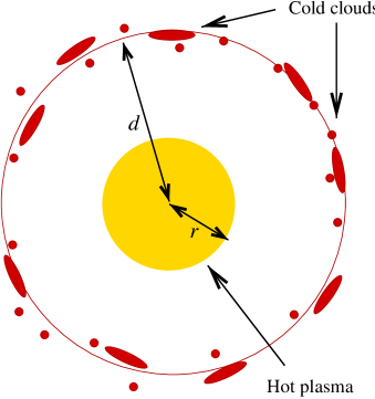
Figure 1: The assumed geometry of the inner accretion flow: the black hole is at the centre of a spherical hot plasma cloud, with radius $r$, forming the hard X-ray source. Cold clouds are spherically distributed at some distance $d$ from the centre. They provide the seed photons for Comptonisation in the hot phase. They intercept a fraction of the primary X-ray radiation. The main part of the intercepted X-ray flux is reprocessed as low energy (UV) radiation, the rest is reflected in the X-ray. The system is assumed to be in radiative equilibrium.

2 Quasi-spherical accretion model

2.1 Setting-up the picture

For the purpose of computing the spectral characteristics, the exact nature of the cold clouds does not need to be specified. They could consist in radially infalling material as well as the residual fragments from the inner part of a disrupted disc orbiting around the central object. We require the accretion flow to be spheric only in its inner parts. This does not preclude the existence of an outer accretion disc. The clouds are even not required to be accreting and they could be part of an outflow or a wind. They are however powered by accretion through reprocessing of the primary hard X-ray radiation.

As long as the number of clouds is large enough the observed spectrum does not depend much on the particular cloud distribution or line of sight. Rather, it depends on general intrinsic characteristics of the source such as the cloud covering fraction and the average relative distance between the clouds and the hot comptonising plasma. The shape of the individual clouds is then indifferent.

Let us consider that the hot phase constitutes a sphere with radius $r$. We note $L_{\rm h}$, the power dissipated inside this hot sphere. We assume that the cold clouds are all at the same distance $d$ from the centre of the sphere (see Fig. 1). We model their effects by assuming that a fraction $C$ of the radiation impinging on the sphere of radius $d$ is intercepted. $C$ is thus the covering fraction of the clouds. A fraction $a$ of the intercepted flux is reflected while the rest is absorbed, reprocessed and reemitted as soft (UV) radiation. $a$ is the energy and angle integrated hard X-ray albedo.

For simplicity, we will assume that all the reprocessed power is emitted by the inner clouds surface, i.e. toward the inner part of the accretion flow. This assumption is reasonable if the clouds are Compton thick and highly absorbing and thermal conductivity can be neglected. Then, most of the impinging energy is absorbed close to the inner surface and reemited locally. In addition to reprocessed emission it is possible that the clouds radiate due to some additional internal dissipation process (see section 4). We will allow for this possibility. We note $L_{\rm d}$ the total power dissipated in the cold clouds and radiated as UV radiation. Half of it is emitted outward, the other half is emitted toward the hot plasma.

The virtual sphere of radius $d$ receives a total power $L_{\rm t}$. It arises from three contributions:

$$L_{\rm t}=L_{\rm x}+L_{R}+L_{\rm uv},$$ (1)

respectively the comptonised luminosity, the reflected luminosity, the soft luminosity. A fraction $CL_{\rm t}$ is intercepted by the reflector and then reprocessed/reflected toward the inner direction. An important quantity is the fraction of luminosity emitted inwardly by the reflector surface which is not comptonised (i.e. emitted toward the reflector without interacting with the hot plasma):

$$K=1-\xi+\xi\exp{-\tau}.$$ (2)

$\tau$ is the hot plasma Thomson optical depth, $\xi=\Delta\Omega/2\pi$ and $\Delta\Omega$ is the solid angle subtended by the hot source as seen from the surface of the reflector. In our spherical approximation, we have:

$$\xi=1-\sqrt{1-\left(\frac{r}{d}\right)^{2}}.$$ (3)

In reality, one expects to have clouds radially distributed around the source, rather than at a given distance. Actually quantities such as $d/r$, $\xi$ or $K$ should be regarded as average quantities, indicative of the characteristic distance where most of the reprocessing takes place. We expect that for most of possible radial distributions one can find an effective $d/r$ that provides a reasonable approximation to the high energy spectrum. The only important effect of a very extended radial distribution would be that a significant fraction of the radiation reprocessed by the outer clouds, rather than feeding the hot phase, escapes trough reflection on the dark side of the innermost clouds. Taking into account this effect would require to introduce a transmission factor for reprocessed radiation which would depend on the specific cloud distribution. In order to limit the number of model parameters and for the sake of simplicity, we will not consider this possibility.

2.2 Model parameters

In the next sections we will link the intrinsic physical and geometric properties of the source to observable quantities. Similar estimates for the luminosity ratios and the amplification factor can be found in a different form in AC00. We extend their results to the case where some dissipation occurs in the cold phase. But the main improvement brought by the present work is to provide estimates for the two measured quantities that are commonly used to describe the hard X-ray spectra, namely the spectral slope $\Gamma$ and the reflection coefficient $R$.

These spectral characteristics are fully determined by 6 parameters: the covering factor $C$, the relative cloud distance $d/r$, the relative dissipation in the clouds $L_{\rm d}/L_{\rm h}$, the hot plasma scattering optical depth $\tau$ and the cloud albedo $a$ and the characteristic energy of the soft seed photons, which may be quantified using an effective blackbody temperature $T_{\rm bb}$.

The albedo depends mainly on the ionization state of matter and also on the shape of the incident spectrum. In the following, we will assume that the cold matter in the clouds is neutral. The characteristic values of the albedo for typical Comptonisation spectra in AGN is then $a\sim 0.1$ (see MBP). Our results are insensitive to its actual value as long as it is low ($a<0.3)$. Since this condition is always realized for neutral matter we will fix $a$$=$0.1 without considering any dependence on the spectral parameters. On the other hand, there is a complication due to our particular geometry which make possible multiple reflections inside the spherical cavity. The neutral albedo for a reflection-like spectrum differs significantly from that for the primary Comptonisation spectrum. We will thus consider a different albedo, noted $a_{R}$, for the reflected luminosity. A Monte-Carlo simulation, considering a typical reflection spectrum incident on neutral matter, provided the value $a_{R}=0.4$ used below.

Precise estimates of $\tau$ from spectral analysis are quite model dependent. In the same object one can infer $\tau$ being as low as a few tenth, and up to a few, depending on the fitting model (Petrucci et al. 2000) and may differ from source to source. However the 2-10 keV spectral slope $\Gamma$ depends only weakly on $\tau$ (see section 2.5 and Fig. 2). The main effect of $\tau$ is on the reflection amplitude $R$ due to the destruction of the reflection component crossing the hot phase (MBP). This effect is important only when the clouds are extremely close to the source (i.e. $d/r<1.1$; see section 3.1 and Fig. 3). Since, $\tau$ is generally found to be of order unity, we will fix the optical depth to the standard value $\tau$=1.

The value of the effective blackbody temperature, $T_{\rm bb}$ affects $\Gamma$ (and also slightly $a$). Changes in $kT_{\rm bb}$ have however almost no effects, as long as they are kept inside the observed range where the bulk of the soft luminosity emerges in AGN (5-50 eV; see Fig. 2). We will thus assume that $T_{\rm bb}$ lies somewhere in that range.

The number of effective parameters is thus reduced to 3, namely: $d/r$, $C$ and $L_{d}/L_{h}$.

2.3 The reflected component

The reflected luminosity $L_{R}$ impinging on the sphere of radius $d$ has been emitted by the reflector itself from a fraction of the impinging X ray luminosity and crossed the system without being Compton scattered, we can thus write:

$$L_{R}=KC(aL_{\rm x}+a_{R}L_{R}).$$ (4)

The additional $L_{R}$ term on the right hand side of equation 4 accounts for multiple reflections in the cloud system.

The amplitude of reflection $R$ is usually defined by the ratio of an observed reflection component to that expected from an isotropic point source with the same luminosity illuminating an infinite slab:

$$R=\frac{L_{R}}{L_{R}^{slab}}.$$ (5)

In our case the latter can be estimated as:

$$L_{R}^{slab}\sim a\frac{L_{\rm x}}{2}f(\cos i).$$ (6)

Indeed, in the disc illumination framework, half of the hard X-ray luminosity is emitted toward the disc, of which a fraction $a$ is then reflected. The angle $i$ is the assumed inclination of the slab. The factor $f(\cos i)$ represents the angular dependence of reflection in the reference slab model. We estimate the $f$ function using the approximation given by Ghisellini et al. (1994):

$$f(\mu)=\frac{3\mu}{4}[(3-2\mu^{2}+3\mu^{4})\ln\left(1+\frac{1}{\mu}\right)+$$

$$(3\mu^{2}-1)\left(\frac{1}{2}-\mu\right)].$$ (7)

It is then straightforward to relate the observable $R$ to the physical parameters of the spherical model:

$$R\sim\frac{L_{R}}{L_{\rm x}}\frac{2}{af(\cos i)}=\frac{2CK}{1-a_{R}CK}f^{-1}(\cos i).$$ (8)

Usually $i$ is a frozen parameter of the fitting model enabling to measure $R$ from comparison to the slab reflection model (cf pexrav model in XSPEC, Magdziarz & Zdziarski 1995). In sections 3 and 4, we will compare the model predictions with the the observational $R$ values given by ZLS99. These data have been fitted with $i$$=$$30^{\circ}$. We will thus adopt this value in most of our numerical estimates.

2.4 The amplification factor

The soft flux incident on the virtual sphere of radius $d$, arises partly from reprocessing on the reflector itself and partly from internal dissipation:

$$L_{\rm uv}=KC\left[(1-a)L_{\rm x}+(1-a_{R})L_{R}+L_{\rm uv}\right]+KL_{\rm d}/2.$$ (9)

The global energy balance can be written:

$$L_{\rm h}+L_{\rm d}/2=(1-C)L_{t},$$ (10)

where $L_{\rm h}$ and $L_{\rm d}$ are the power dissipated in the hot and cold phase respectively. Combining equations 1, 9 and 10 and leads to:

$$L_{\rm uv}=\frac{KC(\omega-a)L_{\rm h}+K(\omega-aC)L_{\rm d}/2}{(1-C)(1-CKa_{R})},$$ (11)

where we set :

$$\omega=1-KC(a_{R}-a).$$ (12)

We defined $L_{\rm uv}$ as the soft luminosity impinging on the virtual sphere. $L_{\rm uv}$ can also be considered as the amount of soft luminosity, inwardly emitted by the reflector, that reaches the sphere of radius $d$ without interacting in the hot plasma. The total soft luminosity emitted by the reflector is thus $L_{\rm uv}/K$. The soft luminosity entering the hot phase is then:

$$L_{\rm s}=\frac{\xi}{K}L_{\rm uv}.$$ (13)

The total luminosity escaping from the hot phase is the sum of the power dissipated internally and the total power received from the cold phase:

$$L=L_{\rm h}+C\xi L_{t}+\xi L_{\rm d}/2.$$ (14)

Then using equation 10, it is straightforward to show that

$$L=\frac{(1-C+C\xi)L_{\rm h}+\xi L_{\rm d}/2}{1-C}.$$ (15)

Finally, combining equation 15 with 11 and 13, we derive an estimate for the amplification factor:

$$A=L/L_{\rm s}=\frac{(1-KCa_{R})\left[(1-C+C\xi)L_{\rm h}+\xi L_{\rm d}/2\right]}{\xi C(\omega-a)L_{h}+\xi(\omega-aC)L_{\rm d}/2}.$$ (16)

2.5 The spectral slope

Figure 2: Relation between amplification factor and photon index $\Gamma$, for a spherical geometry. Soft photons are injected at the sphere surface, with a blackbody spectrum of temperature $T_{\rm bb}$. The symbols show the results of non-linear Monte-Carlo simulations. Open and filled symbols respectively stand for $T_{\rm bb}$=5 and 50 eV. The radial Thomson optical depth of the sphere was fixed to $\tau$=1 (triangles), and $\tau$=0.2 (squares). The solid line shows the approximation given by equation 17 with $\gamma$=2.26 and $\delta$=1/12.

A commonly measured quantity is the photon index $\Gamma$. It represents the spectral slope of the intrinsic Comptonisation power law spectrum (i.e. not including reflection). It is generally measured in the energy range 2–10 keV for a flux given in units of photon per energy (e.g. photon keV^-1 cm^-2 s^-1).

The amplification factor is directly related to the photon index. The $\Gamma$ versus $A$ relation may be derived from numerical simulations. We use the Monte-Carlo code of Malzac & Jourdain (2000) based on the non-linear method proposed by Stern et al. (1995). We consider a sphere of thermal plasma with optical depth $\tau$ defined along its radius. The sphere is homogeneously heated with a power $L_{\rm h}$. Soft photons are externally injected at the sphere surface with a black body spectrum of temperature $T_{\rm bb}$. The injected soft luminosity is $L_{\rm s}$. The density is homogeneous inside the sphere. It is however divided in 10 radial zones in order to account for temperature gradients. For a fixed ratio $L_{\rm h}/L_{\rm s}$=$A$-$1$, the code computes the equilibrium temperature structure as well as the spectrum of escaping radiation. We then use a least-square fit to the 2-10 keV spectrum to determine the photon index $\Gamma$.

Simulations were performed for several values of $A$-$1$ in the range 1–1000, for $T_{\rm bb}$$=$ 5 and 50 eV, $\tau$$=$0.2 and 1. We then discarded simulations resulting in a volume averaged electron temperature larger than 400 keV, i.e. larger than what is inferred from the observations of the high energy cut-off. We also discarded simulations resulting in $\Gamma$ outside of the range of interest regarding to the observations (1.4–2.2). As shown in Fig. 2, this sample of numerical results can be represented by the functional shape proposed by B99b:

$$\Gamma=\gamma(A-1)^{-\delta},$$ (17)

with $\gamma$=$2.26$ and $\delta$=$1/12$.

The largest error is about 7 per cent, arising for $T_{\rm bb}$$=$50 eV, $L_{\rm h}/L_{\rm s}$$=$6 and $\tau$$=$0.2 ($T$$=$360 keV). If one except this high temperature case the error is less than 5 per cent. We conclude that, at least for $\tau$ in the range 0.2–1, and all the other parameters being in the observed range, $\Gamma$ depends (almost) only on the amplification factor. This dependence can be represented with a good accuracy by equation 17.

The value of the coefficient differs slightly from those originally given by B99b ($\gamma$$=$2.33, $\delta$$=$$1/10$). The reasons for these small differences could be that we performed a detailed radiative transfer for the sphere geometry, while Beloborodov’s results are based on a simple escape probability formalism in a one zone approximation (Coppi 1992), and photons injected at the centre. Another possible cause for the discrepancy, is that we fitted numerical results allowing temperature to adjust while temperature was fixed in the calculations of B99b and $\tau$ was varied according to the amplification.

Relation 17, used together with equation 16 relates the observable $\Gamma$ to the model parameters.

Figure 3: Dependence of the spectral parameters on the covering factor $C$. Left panel: $R$ vs $C$; right panel: $\Gamma$ vs $C$. The solid lines stand for the model without dissipation in the cold clouds ($L_{\rm d}$=0), and different distances: $d/r=1,1.2,1.7,2.5$ and $4$ respectively from top to bottom in right panel, from bottom to top in left panel. Dashed lines are for the model with intrinsic dissipation in the clouds such that $L_{\rm d}/L_{\rm h}=60C$ (see section 4). Distances are $d/r=4.0,5.9,9.0,13.6,22.1$ from top to bottom in right panel. In left panel all dashed curves are almost indistinguishable since $R$ is almost independent on $d$ for $d>2$. In all curves the Thomson optical depth is $\tau$=1, cloud albedo is $a$=0.1, reflection angle parameter is $i$=$30^{\circ}$ (see section 2).

2.6 The UV to X luminosity ratio

The observed UV to X-ray flux ratio can be estimated as follow:

$$\frac{F_{\mathrm{uv}}}{F_{\mathrm{x}}}=\frac{(1-C)L_{\rm uv}+L_{\rm d}/2}{(1-C)(L_{\rm x}+L_{R})}.$$ (18)

Then, using equations 9 and 11, one can link the luminosity ratio to the model parameters:

$$\frac{F_{\mathrm{uv}}}{F_{\mathrm{x}}}=\frac{\left(\omega-a\right)KCL_{\rm h}+\left[1+K\omega-KC(a_{R}+a)\right]L_{\rm d}/2}{\omega\left[(1-KC)L_{\rm h}+(1-K)L_{\rm d}/2\right]}.$$ (19)

When comparing to observations one should keep in mind that this relation gives actually only a lower limit on the observed UV to X-ray flux. Indeed, there may be other sources of UV radiation in real objects (like an external accretion disc).

3 Clouds without internal dissipation

In this section, we will assume no dissipation in the blobs ($L_{\rm d}$=0). The solid lines in Fig. 3 show $R$ (left panel) and $\Gamma$ (right panel) as function of $C$ for different ratios $d/r$.

3.1 $R$ versus $C$ relation

The reflection amplitude grows almost linearly with $C$, starting from $R$$=$0 where there is no reflector ($C$=0), and reaching values of order $2$ for fully obscured source ($C\sim 1$). Indeed, as seen from the source, the reflector then covers a solid angle $\sim 4\pi$.

As the observed reflection component is produced on the inner side of the clouds, a fraction of the reflected photons may be Compton scattered in the hot plasma before escaping to the observer. The net effect is to decrease the apparent amount of reflection in the observed spectrum (see MBP). This Compton smearing effect is obviously stronger at low $d/r$, when the hot source subtends a larger solid angle. The maximum $R$ value is then lower, as shown on left panel of Fig. 3. This maximum value depends on the plasma optical depth $\tau$. For an optically thin plasma there is no significant reduction of $R$, while for very thick plasma and very close clouds ($d/r<1.1$) the reflection component can be almost totally destroyed.

On the other hand at large $d/r$ ($>2$), this effect can be neglected. For large covering factors, multiple reflections on the inner side of the clouds tend to increase $R$ up to values larger than 2. In this limit of $d/r$ larger than a few, the shape of the relation $R$ vs $C$ becomes fully independent of $d/r$.

In any case, for reasonable optical depths, the range of achievable $R$ when $C$ varies from 0 to 1, is comparable to the range of observed $R$ (from 0 up to a few).

3.2 $\Gamma$ versus $C$ relation

For very low covering factors ($C\sim 0$) the amplification factor is huge and the spectrum is thus very hard. It softens very quickly with increasing $C$. At $C\sim 0.1$ the growth rate decreases and $\Gamma$ then evolves slowly and almost linearly. The spectral slope softens by $\Delta\Gamma\sim 0.6$ between $C$=0.1 and $C$=0.8. Then, for higher covering factors, the soft radiation emitted by the clouds remain trapped inside the reflector sphere. This effect is non linear, a small increase in $C$ then increases dramatically the amount of soft cooling radiation $L_{\rm s}$ entering the hot plasma. As a consequence the emitted spectrum softens very quickly and $\Gamma$ diverges again for $C\sim 1$.

The effect of changing $d/r$ does not change significantly the global shape described above. Increasing $d/r$ simply shift the curve downward. Indeed, the feedback from the clouds decreases, as they are more distant, and the spectra are harder on average.

For clouds distances in the range $r$$<$$d$$<$$4r$ the plateau of the curve falls in the range $1.4<\Gamma<2.2$. The observed range of $\Gamma$ values is then produced with intermediate $C$ values ($0.1<C<0.8$).

3.3 $R$ versus $\Gamma$ relation

As both $R$ and $\Gamma$ increase with $C$, it is obvious that changes in the covering factor will produce a correlation between these two spectral parameters. It is then interesting to compare this correlation with the observed one.

The solid lines in Fig. 4 show the $R$-$\Gamma$ correlation obtained when varying the covering factor of the source. The data points (from ZLS99) are also plotted in this figure. The different curves are for different fixed values of the distance $d$ from the centre. Clearly, the overall shape of the correlation is well reproduced as long as the reflector is closer than 3 times the size of the X-ray source. Most of the data points lie in this range. This range of distances could be the dispersion of the average distance of the reprocessor in different sources. It is also probable that most of the apparent spread is simply due to errors in the measurements of $R$ and $\Gamma$.

If the reflector is located at distance larger than $\sim 3r$ the feedback from reprocessing becomes too low and this produces very hard spectra. The distance is thus strongly constrained to be below $3r$. If some dissipation occurs, however, a wider range of distances is allowed, see section 4.

The prediction of a correlation, as well as its general shape, are insensitive to our model assumptions.

3.4 Distributions in the $d/r$-$C$ plane

The system formed by equation 8, 16 and 17, giving $R$ and $\Gamma$ as a function of $d/r$ and $C$ is, in general, invertible analytically. It is thus possible to transpose the $R$-$\Gamma$ data shown in Fig. 4 into the $d/r$-$C$ plane. The result is shown in Fig. 5. It illustrates the fact that the values of the distance are comparable from source to source, while the covering factor can change by a large amount. In the passive case the average distance is $<$$d/r$$>$=1.7, the root mean square spread is about 35 per cent.

For a fixed $L_{\rm d}/L_{\rm h}$, the correspondence between any couple ($R$, $\Gamma$ ) and ($d/r$, $C$) is univocal as long as $R$$\neq$0. If $R$$=$0 then $C$$=$0, and $d/r$ is undetermined. Several data points of our sample fall into this unphysical case. The probable reason is that the reflection component was too weak to be detected. Then we can infer that $C$ is actually very low, but $d/r$ cannot be estimated at all. Therefore such data are not represented in Fig. 5.

On the other hand, we used them for the purpose of computing the observed distribution of covering factors $p(C)$, displayed in Fig. 6. Clearly, the $C$-distribution appears to be a decreasing function of $C$. As shown in Fig. 6, it is reasonably well represented by a linear distribution i.e.:

$$p(C)=2(1-C).$$ (20)

This distribution has the same average value as the observed one: $<$C$>$=0.33. The distribution $p(C)$ represents the probability density of observing a source with a covering factor $C$. It does not necessarily reflects the intrinsic distribution of covering factors, since $p(C)$, the distribution of observed $C$, is likely to include some selection effects.

3.5 $R$ and $\Gamma$ distributions

Assuming a fixed $d/r$, for a given $C$-distribution $p(C)$ the respective distribution of $R$ and $\Gamma$ are respectively given by :

$$p_{R}=p(C)\left(\frac{{\rm d}R}{{\rm d}C}\right)^{-1},$$

$$p_{\Gamma}=p(C)\left(\frac{{\rm d}\Gamma}{{\rm d}C}\right)^{-1}.$$ (21)

For a given $p(C)$, an analytical expression for $p_{R}$ and $p_{\Gamma}$ can be easily derived from equations 8 and 16.

The solid lines in Fig. 7, compare the predicted $p_{R}(R)$ and $p_{\Gamma}(\Gamma)$ for $p(C)$ given by equation 20 with the observed distribution. They are qualitatively reproduced for $d/r$$=$$<$$d/r$$>$=1.7. This confirm that the actual $p(C)$ is well represented by the equation 20.

It is striking to have such a good agreement despite we neglected the spread in $d/r$. Actually, the shapes of $p_{R}(R)$ and $p_{\Gamma}(\Gamma)$ are not very sensitive to the value of $d$, as long as it is kept in the observed range. A reasonable agreement is obtained as long as 1.3$<$$d/r$$<$2. Only for very close reflector, the effects of Compton smearing of the reflection component become important. The $R$ distribution steepens slightly, with, on average lower $R$ values. Concerning $p_{\Gamma}$, at larger $d$, the average $\Gamma$ is harder, and the distribution is slightly narrower.

Unlike the $C$-distribution, the theoretical $\Gamma$ distribution depends somewhat on the exact relation between $\Gamma$ and the amplification factor $A$. Different approximations used to represent this exact relation may give different results. For example, if instead of equation 17 with $\gamma$$=$2.26, $\delta$$=$1/12, we use the coefficients given by B99b (i.e. $\gamma$$=$2.33, $\delta$$=$1/10) we get a larger width and softer spectra. If instead we use $\gamma$$=$2.15, $\delta$$=$1/14, as given by MBP for a cylindric geometry, we get, on the contrary, a distribution with a smaller width, peaking at harder spectra. In both cases, the shape of the distribution is still in qualitative agreement with the data.

We conclude that the spread in $d/r$ is actually negligible and the $C$-distribution plays a major role for the observed $R$ and $\Gamma$ distributions. Simply by setting the only significant parameters (namely $d/r$) to a value relatively close to 1.7, the model qualitatively reproduces three observational pieces of information that we have on the sources: the correlation $R$-$\Gamma$, and the respective distributions of $R$ and $\Gamma$.

3.6 Distribution of UV to X flux ratios $F_{\mathrm{uv}}/F_{\mathrm{x}}$

Using equation 19, one can derive the distribution of the $F_{\mathrm{uv}}/F_{\mathrm{x}}$ that is predicted by the model with the $C$-distribution given by equation 20. The solid line in Fig. 8 shows the theoretical distribution which is compared with the observed one (data from Walter & Fink 1993). This kind of comparisons should be taken with caution, since the expression for $F_{\mathrm{uv}}/F_{\mathrm{x}}$ given by equation 19 refers to integrated quantities while the measurements of Walter & Fink were performed at a fixed UV and X-ray wavelengths (respectively 1375 Å and 2 keV). Moreover, as shown by Kuncic et al. (1997), small clouds probably emit in the EUV, rather than in the UV.

Despite these uncertainties, Fig. 8 clearly shows that the modeled and observed distributions do not match. For $F_{\mathrm{uv}}/F_{\mathrm{x}}$ larger than a few, the model probability density is very close to 0. In contrast, the observed distribution extends up to quite large large UV to X flux ratios ($F_{\mathrm{uv}}/F_{\mathrm{x}}\sim 50$). Clearly, the inner clouds do not emit enough UV radiation to reach the highest observed UV to X luminosity ratios. Note that, in principle, the model can produce arbitrarily large $F_{\mathrm{uv}}/F_{\mathrm{x}}$ (see equation 19), by setting $C$ and $K$ close to unity. The problem is that it produces a too small amount of large $F_{\mathrm{uv}}/F_{\mathrm{x}}$ sources. Fitting the observed $F_{\mathrm{uv}}/F_{\mathrm{x}}$ distribution would require a distribution of covering factor which would be a growing function of $C$, in contradiction to what is inferred from the X-ray data.

In an attempt to solve the problem, one can think about considering that a fraction of the reprocessed flux is transmitted through the cloud instead of being fully emitted toward the hot plasma (see AC00). However, this does not increase the observed $F_{\mathrm{uv}}/F_{\mathrm{x}}$ ratio. In fact, the opposite occurs. Due to the additional losses, amplification of the UV field in the cloud cavity is less efficient and, for a given covering factor, the observed $F_{\mathrm{uv}}/F_{\mathrm{x}}$ ratio is lower.

This apparent discrepancy can be overcomed if one consider that we assumed that all the soft radiation is produced trough reprocessing of the hard X-rays, without any additional source of UV radiation. The data simply suggest that such additional sources of UV radiation are present in real sources. These sources of UV radiation could be external, and not directly related to the central cloud system. For example, an external disc could be responsible for a significant (if not the largest) fraction of the observed UV emission. Then, the expected distribution UV to X luminosity ratio will depend on additional parameters such as the disc inner radius or inclination. Estimating the $F_{\mathrm{uv}}/F_{\mathrm{x}}$ distribution would require additional assumptions and several physical complications. From a qualitative point of view however, it is obvious that the resulting distribution would extend up to larger $F_{\mathrm{uv}}/F_{\mathrm{x}}$, as required by the data.

Such an outer source of UV radiation is unlikely to contribute sensibly to the cooling of the central source neither to the reflected component. Thus, our estimates for $R$, $\Gamma$, $p_{R}$ and $p_{\Gamma}$ are still valid, as well as our conclusion drawn from the comparison with data: the present model enable to explain the main properties of the hard X-ray continuum observed in Seyfert galaxies provided that the passive clouds are distributed at distances $d$, in the range $r$–3$r$ from the central hot plasma region of radius $r$.

Another possibility is that the additional source of UV luminosity would be located in the cold clouds themselves. Then, the excess soft luminosity may affect the radiative equilibrium and subsequently the emitted spectrum. We thus have to take it into account when computing the spectral characteristics and distributions. This, in turn, requires some additional assumptions on the energy dissipation process presumed to be active in the clouds. Then however, it makes it possible to build a simple self-consistent model accounting for the UV to hard X-ray spectral properties of the continuum emitted in Seyfert galaxies. This is the aim of the next section.

Figure 4: The predicted $R$-$\Gamma$ correlation compared with observations of Seyfert galaxies. The circles are the best fits parameters to the Ginga data (Zdziarski et al. 1999) in the $R$ vs $\Gamma$ plane. The lines represent the correlation obtained for cold blobs are at a fixed distance from the hot plasma and covering fraction varying from 0 to 1. The solid lines stand for models with negligible dissipation in the blobs, from left to right for $d/r$=4, 2.5, 1.7, 1.2, and 1, respectively. The dashed lines stand for models with dissipation in the cold medium proportional to the covering factor $L_{\rm d}/L_{\rm h}=60C$ (see section 4). The assumed distances from the centre are 22.1, 13.6, 9.0, 5.9, 4.0 times the size of the hot plasma, respectively from left to the right hand side. The Thomson optical depth is fixed to unity, the reflector albedo is $a$=0.1, the reference inclination angle for reflection (see text) is $i$$=$$30^{\circ}$. The corresponding covering factors can be estimated from Fig. 3.

Figure 5: The same $R$-$\Gamma$ data as in Fig. 4, transposed into the $d/r$ vs $C$ plane. The position of the open circles was determined assuming no dissipation in the cold phase ($L_{\rm d}/L_{\rm h}$$=$0), while $L_{\rm d}/L_{\rm h}$$=$60$C$ was assumed for the filled circles. The Thomson optical depth is fixed to unity, the reflector albedo is $a$$=$0.1, the reference inclination angle for reflection (see text) is $i$$=$$30^{\circ}$. Data with $R$=0 were excluded (see text).

Figure 6: The observed distribution of the covering factors. The histograms were determined using the data (Zdziarski et al. 1999). The lines show fits to histograms assuming $p_{C}(C)=(1+\alpha)(1-C)^{\alpha}$. $\alpha$ best fitting values are $1$ and $1.5$ respectively in the passive case (solid lines, $L_{\rm d}/L_{\rm h}$=0) and in the active clouds case (dashed lines, $L_{\rm d}/L_{\rm h}=60C$). The Thomson optical depth is fixed to unity, the reflector albedo is $a$=0.1, the reference inclination angle for reflection (see text) is $i$=$30^{\circ}$.

4 Clouds with internal dissipation

Figure 7: Comparison of the predicted spectral parameters distribution with the observed one. Left panel: the $R$ distribution, right panel the $\Gamma$ distribution. The histograms show the observed distributions in the sample of Zdziarski et al. (1999). Solid lines shows the model predictions for $L_{\rm d}$=0, $d$=1.7 $r$. The dashed line show the model predictions for $L_{\rm d}/L_{\rm h}=60C$ and $d$=8.5$r$ (see section 4). The assumed distributions of covering factors are those shown in Fig. 6. The Thomson optical depth is fixed to unity, the reflector albedo is $a$=0.1, the reference inclination angle for reflection (see text) is $i$=$30^{\circ}$.

4.1 Dissipation process

There may be some mechanism providing a substantial dissipation in the cold medium, even if we consider spherical accretion. An example of such mechanism is turbulent dissipation at shocks (Chang & Ostriker 1985) that are likely to form due to the development of spatial instabilities (Kovalenko & Eremin 1998). It is out of the scope of this paper to discuss or model accurately the dissipation mechanism. The only assumption that we will make about the dissipation process, is that the total relative power dissipated in the cold phase grows linearly with the covering factor i.e.:

$$\frac{L_{\rm d}}{L_{\rm h}}=\eta C.$$ (22)

It is indeed quite natural to assume that dissipation increases with the amount of matter in the cold phase. This is also required by the existence of the $R$-$\Gamma$ correlation. Our prescription consists in choosing the simplest (linear) function enabling to produce a $R$-$\Gamma$ correlation. The $\eta$ coefficient represents the highest relative dissipation possible in the cold phase. It is obtained for a fully covered source. In the following, we will assume that $\eta$ is a (nearly) universal constant. We will consider it as a free parameter and try to get some constraints with the data.

4.2 Effects of internal cloud dissipation on $\Gamma$ and $R$

It is obvious that increasing the internal dissipation parameter $\eta$, will have a similar effect on $\Gamma$, as decreasing the distance ratio $d/r$. In both cases, the cooling soft radiation flux entering the hot phase becomes larger, the amplification factor diminishes and the spectrum softens.

As the effects of both parameters almost compensate, very similar $\Gamma(C)$ curves may be obtained for very different values $\eta$ and $d/r$ provided they are adjusted together in order to keep $\Gamma(C)$ unchanged. One can derive a simple relation between $\eta$ and $d/r$ enabling to conserve $\Gamma(C)$. Indeed, expression 16 for the amplification factor can be rewritten using the prescription of equation 22:

$$A=\frac{1-\left[1-\xi\left(1+\eta/2\right)\right]}{\xi\left(1+\eta/2\right)C}.$$ (23)

For simplification, in this expression, second order effects due to reflection have been neglected (i.e. we set $a$$=$0). Equation 23 shows that at first order, the function $A(C)$ and thus $\Gamma(C)$ will remain unchanged provided that the quantity:

$$\xi_{0} = \xi(1+\eta/2)$$ (24)

$$= \left(1-\sqrt{1-\left(\frac{r}{d}\right)^{2}}\right)(1+\eta/2),$$

is kept constant. $2\pi\xi_{0}$ is the value of the solid angle subtended by the hot phase as seen from the reflector that provide the same $\Gamma(C)$ curve without internal dissipation in the cold phase ($\eta$$=$0).

The solid lines, in the right panel of Fig. 3, show different $\Gamma(C)$ curves obtained for different distance ratios $d/r$ and no cloud dissipation ($\eta$$=$0, see section 3.2). For each solid line, we computed a model with internal dissipation in the clouds shown in dashed line. We fixed $\eta$$=$60 (this value will be shown to fit the $F_{\mathrm{uv}}/F_{\mathrm{x}}$ distribution in section 4.4), and $d/r$ was computed according to equation 24, with $\xi_{0}$ determined from the distance parameter of the corresponding non dissipative model. Solid and dashed curves are very close from each other. There are only minor differences due to effects of reflection. The global properties of the $\Gamma$ vs $C$ relation are thus unchanged when dissipation in the cold clouds is taken into account. Only the distance-scale is different.

From equation 21, one can see that $R$ is fully independent of $\eta$. And, as quoted in section 3, $R$ is almost independent of $d$, specially when $d$ is large. This can be seen on the left panel of Fig. 3, the dashed curves show the $R$ versus $C$ relation for different distances ($d/r$$>$4), corresponding to those of the right panel. They are almost indistinguishable from each other. The model will always produce the correct range of $R$ values.

Then, the shape of the predicted $R$-$\Gamma$ correlation at constant $d/r$, appears to be nearly unchanged provided that $d$ and $\eta$ are tuned simultaneously according to equation 24. In Fig. 4, the dashed lines show the model $R$-$\Gamma$ correlation for $\eta$$=$60. One can see that the observed correlation is then reproduced for reflector distances in the range $4r<d<14r$. At the lowest limit, the strong dissipation in the cold phase cools the plasma down to very low temperatures and the spectra are too soft, on the other hand, large $d$ values produce too hard spectra.

4.3 Effects of internal cloud dissipation on the $C$ and $d/r$ distributions

When dissipation is assumed, the data points, considered in the $d/r$-$C$ plane, shift toward larger $d/r$. The shift in distance can be estimated using equation 24. Indeed, we know from section 3 that for $\eta$$=$0 the average distance is $d/r$$=$1.7. Thus, fixing

$$\xi_{0}=1-\sqrt{1-(1/1.7)^{2}}\sim 1/5,$$ (25)

in equation 24, provides the general relation between $\eta$ and $d$ which enables to fit the observed $\Gamma$ distribution. In the limit of large distances, (effectively $d>3r$) expression 24 with $\xi_{0}$$=$1/5 becomes

$$\frac{d^{2}}{r^{2}}\sim\frac{5}{4}\eta.$$ (26)

This can be understood geometrically as being (for large $d$) a relation enabling a constant average soft photon input in the hot phase when varying $d$ (or $\eta$). It may also tell us that the dissipation process has to provide a fixed amount of dissipation per unit surface of reflector. The numerical constant in front of the relation is close to unity. This indicates that we need nearly the same amount of dissipation per unit surface, both in the reflector and the hot medium.

The data distribution in the $d/r$-$C$ plane for $\eta$$=$60, is shown in Fig. 5. At first sight, the points are simply shifted toward larger $d/r$ as compared to the passive case. The average distance is $<$$d/r$$>$=8.5, in agreement with equation 26. The root mean square spread around the average is 44 per cent.

A more detailed inspection of Fig. 5 reveals that the data points are slightly shifted toward the left (i.e. lower $C$) compared to the passive case. This shift is due to the slight dependence of $R$ on $d/r$. It affects the $C$-distribution shown in Fig. 6. Equation 20 provides only a poor approximation to the observed $C$-distribution with dissipation. Instead, the following function:

$$p(C)=(1+\alpha)(1-C)^{\alpha},$$ (27)

with $\alpha$=1.5, gives a good representation of the distribution (see Fig. 6).

We fitted the observed $p(C)$ distribution, for different values of $\eta$, with the function 27 and $\alpha$ as a free parameter. The resulting best fitting values are close to unity as long as $\eta$ is low $<1$, for larger $\eta$, $\alpha$ converge quickly toward 1.5. For any $\eta>$10 the $C$-distribution is well represented by equation 27 with $\alpha\sim$1.5. We checked that these results are not significantly affected by statistical errors due to a particular bining of the $C$-distribution.

In all cases the derived $p(C)$ distribution provided a reasonable agreement with the $R$ and $\Gamma$ distributions, as long as $d/r$ is set to the average value given by the data. Fig. 7 illustrates the case $\eta$=60 with $d/r$=8.5, comparing the derived $R$ and $\Gamma$ distributions with the data in a way similar to that of section 3.5. As expected, they are very well reproduced.

4.4 $F_{\mathrm{uv}}/F_{\mathrm{x}}$ distribution

The observations provide an upper limit on $\eta$. Indeed in the limit of large $\eta$, this parameter is roughly comparable to the largest UV to X-ray luminosity ratio predicted by the model. As a consequence, $\eta$ can not be much larger than the maximum observed UV to X fluxes ratios. It turns out (see e.g. Fig. 8) that the largest observed UV to X ratios are in the range 10-100. This observational fact constrains $\eta<100$. As a consequence of equation 26, this limit indicates that the reflector cannot be at a distance larger than $\sim 13r$.

Fig. 8 shows that the observed $F_{\mathrm{uv}}/F_{\mathrm{x}}$ distribution in Seyfert 1 galaxies is well represented by the model with $\eta$=60 (dashed line). This result is not very sensitive to $\eta$ as long as it keeps being comparable to the largest observed $F_{\mathrm{uv}}/F_{\mathrm{x}}$ values. Reasonable agreement with the observed distribution can be achieved for $40<\eta<80$. The predicted distribution is insensitive to reflector distance as long as $d>3r$.

We stress again that the distribution of the observed $F_{\mathrm{uv}}/F_{\mathrm{x}}$ does not provide any lower limit on $\eta$, which can be much smaller than 60, the limiting case $\eta$=0 was studied in section 3. Then, however, external sources of soft radiation are required in order to explain the important amount of sources with large $F_{\mathrm{uv}}/F_{\mathrm{x}}$ ratios.

We conclude that fixing the universal relative dissipation to be roughly $L_{\rm d}/L_{\rm h}\sim 60C$, and the distance $d\sim 8.5r$, enable to explain the $R$ and $\Gamma$ distribution, their correlation and, independently the observed distribution of $F_{\mathrm{uv}}/F_{\mathrm{x}}$. This result is not very sensitive to the exact value of the parameters: a qualitative agreement can be achieved in a quite large region of the parameter space.

Figure 8: Comparison of the predicted $F_{\mathrm{uv}}/F_{\mathrm{x}}$ distribution with the observed one. The histogram shows the observed distribution in the sample of Walter & Fink (1993). The curves show the model distribution computed according to equation 18 and assuming the distributions of covering factors shown in Fig. 6. The solid line is for a reflector distance $d$=1.7$r$ without any dissipation in the clouds: additional sources of UV radiation are required to explain the observed distribution (see section 3.6). Dashed line is for $d$=8.5$r$ and a relative dissipation in the clouds such that $L_{\rm d}/L_{\rm h}=60C$ (see section 4): the UV emission can be understood as being totally emitted by the cold clouds. In both cases optical depth is $\tau$=1, the cloud albedo is $a$=0.1 (see section 2).

5 Additional considerations

5.1 Absorption features

The observed column density of absorbing cold material on the line of sight of Seyfert 1 galaxies is usually quite weak ($N_{H}\mathrel{\hbox{\raise 2.15277pt\hbox{$<$}\hbox to0.0pt{\hss\lower 2.15277pt\hbox{$\sim$}}}}10^{21}$ cm^-2). As already quoted by Celotti et al. (1992) this may indicate that the cloud column density is low. A larger amount of absorbing material would induce a characteristic hardening of the spectral slope in the soft X-ray, since the lower energy photons are more likely to be absorbed than harder ones. Such an absorption feature would be easily detected.

However, our comparisons with the data have shown that, at least for some sources, large covering factors are required. A low absorbing column density is not compatible with a large fraction of primary radiation being intercepted (up to 80–90 per cent). A possibility would be, on the contrary, to have the clouds optically very thick (i.e. highly absorbing, $N_{H}\sim 10^{25}\quad\mathrm{cm}^{-2}$). So that, the fraction of escaping X-ray luminosity intercepting the clouds would be fully blocked, while the rest would escape without any spectral alteration.

The constraints on the clouds column density are less stringent at low covering factor. Then, the effects of absorption on the observed spectrum are weak in any case. The observed $R$ and $\Gamma$ distributions suggest that most of the sources are observed with a low covering factor. According to the distribution 20, 75 per cent of the observed objects would have $C<0.5$. Thus, for most of the observed sources the cloud optical thickness may be low. When the amount of darkening material is increased, it is likely that the additional matter spreads in the three dimensions, so that its radial optical depth grows together with the surface covered.

Still, the absorption effects might be observable in some sources, with large covering fractions i.e. very steep power law spectrum. At low energy ($<$ 10 keV) the radiation escapes only through the uncovered parts of the source. Above 20 keV the clouds are transparent to radiation, the observed 20-30 keV flux could be larger than the extrapolation of the 2-10 keV one, by nearly an order of magnitude. This would induce a strong hardening of the spectrum similar to what is observed in some obscured Seyfert 2 galaxies. Since such a characteristic is specific to the quasi-spherical accretion scenario, a detailed investigation of the soft gamma-ray spectrum of the softest Seyfert 1 galaxies would be of great interest. However, even at high energy, the radiation still suffers Compton down scattering on the cold matter. If the cloud Thomson optical depth is large, the energy loss is important and the down scattered radiation is absorbed before escaping from the cloud. This may limit the observability of the absorption features.

5.2 Is the observed $C$-distribution due to selection effects ?

If, as suggested in section 5.1, the clouds are highly absorbing, it may arise that in some objects, the X-ray source is completely hidden, either because one large cloud is on the line of sight, or because a particular cloud distribution happens to fully cover the X-ray source as seen from earth. Obviously such sources would be very unlikely to be detected. Such an effect may explain that according to the $C$ distribution derived from the data, we observe much more sources with a low covering factor than highly covered ones.

Indeed, for a nearly homogeneous intrinsic $C$-distribution, and if, for the observer, the angular size of an individual cloud, is much larger than the hot source size (i.e. in the limit of extended clouds at large distances), the probability of detecting a source decreases exactly like its uncovered fraction $(1-C)$. In the general case, the exact $C$-distribution depends on the average number of clouds, and their distance and size distributions. In addition, both size and number are likely to be a function of $C$. Depending on the details, one can reasonably get a distribution decreasing more or less according to $(1-C)^{\alpha}$ with $\alpha$ in the required range.

This kind of extinction effects are more likely to occur if the cloud distance is large. Simple geometrical considerations show that a complete extinction is possible only when $(r/d)^{2}>(2c-c^{2})^{-1/2}$. Even above this limit, strong departure from spherical geometry may be required. Such effects are thus unlikely to be important at low $d/r$ (i.e.if there is no dissipation in the clouds). On the other hand, the observed $C$-distribution may be strongly affected by such selection effects if the clouds are at a larger distance, i.e. $d/r>3$, as considered in section 4.

In the case where the source of primary emission is hidden, it might be detected in the X-rays through the reflected radiation coming from the clouds themselves. Thus, if obscuring effects are important, we can expect to detect some very faint sources with infinite reflection coefficient. Such detections have not been reported. However, at least one previously known and usually bright source (NGC4051; Guainazzi et al. 1998) has been observed in a very faint state dominated by reflection. Such spectrum can be interpreted as being due to a obscuring event.

The obscuring clouds of the present model cannot be identified with the obscuring material that hide the broad line region (BLR) in Seyfert 2 galaxies. The BLR is at large distance from the black hole ($>10^{3}$ gravitational radius $R_{g}$), so the obscuring material is, at least, at a similar distance. On the other hand our clouds are constrained to be in the very inner part of the accretion flow ($<100$ $R_{\mathrm{g}}$).

Figure 9: The $R$-$\Gamma$ data of Gilfanov et al. (2000) for galactic black holes, transposed into the $d/r$ vs $C$ plane. Circles, triangles and squares represent data for Cygnus X-1, GX 339-4 and GS 1354-644 respectively. There is no dissipation in the cold phase ($L_{\rm d}/L_{\rm h}$=0). The Thomson optical depth is fixed to unity. The reflector albedo is larger for GBH than AGN (see MBP), we set $a$=0.15. Following GCR00, the reference inclination angle for reflection (see text) is set to $i$=$50^{\circ}$. The coefficients of B99b ($\gamma$=2.33, $\delta$=1/6) relevant for GBH are used in equation 17.

5.3 Galactic black holes

Since GBH sources present hard X-ray spectral properties which are very similar to those of Seyfert 1 galaxies, this model can, in principle, be applied to such objects. We compared the predicted correlation with the data given by GCR00. In these comparisons, the $\Gamma$ versus $A$ relation was approximated by equation 17 with coefficient $\gamma$ and $\delta$ appropriate for GBH. We used both coefficients given by B99b ($\gamma$=2.33, $\delta$=1/6) and MBP ($\gamma$=2.19, $\delta$=2/15). In both cases, we found a reasonable agreement with the observed $R$-$\Gamma$ correlation for $d$ in the range 1.1–1.4, without dissipation in the clouds. Fig. 9 shows the data of GCR00 represented in the $d/r$-$C$ plane. The average $d/r$ value is 1.2. The rms $d/r$ spread is about 4 per cent, much smaller than in the extra-galactic case.

The distribution of spectral parameters is found to be inconsistent with a covering factor distribution of the type given by 27. The sample of data of GCR00 contains only 3 sources (Cygnus X-1, GX 339-4 and GS 1354-644) with numerous observations of each source. This situation differs from the Seyfert sample where we have a larger amount of sources (23) with less observations of each sources (2 on average). In GBH, we trace the physical evolution of a few particular sources, while in Seyfert galaxies, we trace the properties of the whole class. In Seyfert galaxies also, selection effects are more likely to bias the distribution. Therefore, the source statistic is expected to be different.

It is not clear if such a spherical model could explain the complex temporal behavior of galactic sources, whose interpretation generally requires the presence of a disk very close to the central object. Actually, the striking spectral similarities between GBH sources and Seyfert galaxies (similar hard X-ray spectra, correlation R-$\Gamma$), are probably due to the universal properties of Compton self-regulated plasma. The underlying heating process and geometry could be however very different.

5.4 The iron line profile

We focussed on the properties of the continuum spectra and did not attempt to model any line emission. It is however worth mentioning the iron K$\alpha$ fluorescence line at 6.4 keV. Such lines are indeed commonly observed in Seyfert galaxies (Nandra & Pounds 1994; Nandra et al. 1997). They generally present a broad, possibly red-shifted profile. The usual interpretation is that the line forms trough illumination of the innermost part of an accretion disc. The line profile then appears broadened and red shifted due to special and general relativistic effects (Fabian et al. 1989; Tanaka et al. 1995). It seems however that some alternative mechanisms may produce the broad line profiles without a disc (see Karas et al. 2000, and references therein). Such mechanisms include:

1. Radiative transfer effects, like reflection by a ionized medium with an intermediate temperature ($kT\sim 1$ keV). This warm medium could be the transition region located between the hot phase and the cold clouds.

2. Doppler effects due to cloud motions. For example, if the clouds form an out-flowing wind. The line is formed by reflection on the inner side of the clouds traveling away from the observer. It is then Doppler red-shifted and broadened due to the spread in the clouds radial velocities.

3. Gravitational red-shift, if the size the system is small enough.

Or a combination of these different effects. Note also that a recent reanalysis of the ASCA data (Lubiǹski & Zdziarski 2000) indicates that in most of sources, the broadening is much less important than previously thought.

5.5 Ionization

We assumed that the clouds are dense enough so that the ionization parameter is low ($<10^{3}$) and the ionization effects are weak (e.g. Życki et al. 1994). Then, the cloud albedo is low $a\sim 0.1$ and most of the hard X-rays impinging on the clouds are absorbed.

For large ionization parameter a ionized skin forms on the irradiated surface of the clouds. Such ionization may have important effects on the radiative equilibrium (Ross, Fabian & Young 1999; Nayakshin, Kazanas & Kalman 2000) and change many observational parameters such as the hard X-ray spectral slope, the amplitude of the reflection component or the UV to X-ray luminosity ratio. Despite we restricted our considerations to neutral clouds, most of our analytical estimates, given in section 2, may be used to study ionized cases, simply by setting the cloud albedo to a convenient value.

Only equation 8, giving the reflection amplitude, would breakdown. Indeed, the $R$ parameter, as measured in spectral fits gives the amount of reflection on a nearly neutral matter. Reflection on strongly ionized material produces a spectrum which is indistinguishable from the primary emission. Our estimate gives the truly reflected luminosity both on neutral and ionized matter. Equation 8 thus overestimates the effective $R$ when ionization is important.

6 Conclusion

We assumed a spherical distribution of reflecting/absorbing matter surrounding the central source of primary radiation in Seyfert galaxies. We showed that such a situation is consistent with the $R$-$\Gamma$ data. The model successfully reproduces the range of observed spectral slopes and reflection amplitudes, the $R$-$\Gamma$ correlation and the individual $R$ and $\Gamma$ distributions. The same model is also consistent with the $R$-$\Gamma$ data of galactic black holes.

The two main quantities controlling the value of the spectral parameters are the average cloud distance to the hot plasma size ratio $d/r$, and the covering factor $C$. The observations of Seyfert galaxies put the following constraints on the model parameters:

1. The data indicate that the distance $d/r$ of the cold material is comparable in all objects. On the other hand, wide changes in the covering factor $C$ from source to source would be responsible for the observed spectral differences.

2. The observed distributions of spectral parameters require the distribution of covering factors to decrease with $C$. A $C$-distribution of the form $p(C)=(1+\alpha)(1-C)^{\alpha}$ with $\alpha$ in the range 1–1.5, gives a good description of the data. If $d$ is large ($d>3r$) this kind of distribution may be explained by darkening effects. Otherwise, if $d<3r$, it is more likely that the observed $C$-distribution reflects the intrinsic one.

3. Without dissipation in the cold phase: the clouds are constrained to be in the immediate vicinity of the central hot plasma. The data indicate an average relative distance $<$$d/r$$>$=1.7 with a small spread in distance from source to source. The index $\alpha$ of the $C$-distribution is 1.

4. If there is some internal dissipation in the soft phase, growing proportionally to $C$ ($L_{\rm d}/L_{\rm h}=\eta C$): the cloud distance may be larger, depending on the amount of dissipation in the cold phase. For $d>3r$, the average distance required by the data grows with $\eta$, like $d/r\sim\sqrt{1.25\eta}$.

5. In any case the distance is constrained to be lower than $d\sim 13r$, by the maximum observed UV to X flux ratios. Fixing $d\sim 8.5r$ (and $\eta\sim 60$) enables us to understand the bulk of the UV emission as being emitted by the spherical reflector itself. Then, the index of the $C$-distribution, derived from the X-ray data, is $\alpha$$=$1.5. The distribution of $F_{\mathrm{uv}}/F_{\mathrm{x}}$ ratios derived from this $C$-distribution is consistent with the observed one. If the cloud distance is lower than 8.5$r$, the $F_{\mathrm{uv}}/F_{\mathrm{x}}$ data suggest that part of the observed UV flux is emitted by some additional source, external to the cloud system.

This simple model, with a limited number of parameters, enables us to understand the bulk of the phenomenological properties of the continuum emitted in Seyfert 1 galaxies. We believe this is a strong support in favor of a spherical inner accretion flow in these sources.

References

- [] Abrassart A., Czerny B., 2000, A&A, 356, 475 (AC00)
- [ ] Beloborodov A. M., 1999a, ApJ, 510, L123
- [ ] Beloborodov A. M., 1999b, in Poutanen J., Svensson R., eds, ASP Conf. Series Vol. 161, High Energy Processes in Accreting Black Holes. Astron. Soc. Pac., San Francisco, p. 295 (B99b)
- [] Beloborodov A.M., 2001, “Accretion disk models for luminous black holes”, 33rd COSPAR Assembly, to appear in Adv. Space Research, astro-ph/0103320
- [ ] Bisnovatyi-Kogan G.S., Blinnilov S.I., 1977, A&A, 59, 111
- [ ] Celotti A., Fabian A.C., Rees M.J., 1992, MNRAS, 255, 419
- [ ] Chang K.M., Ostriker J.P., 1985, ApJ, 288, 428
- [] Collin-Souffrin S., Czerny B., Dumont A.-M., Zycki P. T., 1996, A&A, 314, 393
- [] Collin S., Abrassart A., Dumont D., Mouchet M., in proc. ”AGN in their Cosmic Environment”, Eds. B. Rocca-Volmerange & H. Sol, EDPS Conf. Series in Astron. & Astrophysics, in press, astro-ph/0003108
- [ ] Coppi P.S., 1992, MNRAS, 258, 657
- [] Czerny B., Dumont A.M., 1998, A&A, 338, 386
- [ ] Fabian A.C., Rees M.J., Stella L., White N.E., 1989, MNRAS, 238, 729
- [ ] George I.M., Fabian A.C., 1991, MNRAS, 249, 352
- [ ] Ghisellini G., Haardt F., Matt G., 1994, MNRAS, 267, 743
- [ ] Gilfanov M., Churazov E., Revnivtsev M., 2000, in Proc. 5th CAS/MPG Workshop on High Energy Astrophysics, in press, astro-ph/0002415 (GCR00)
- [ ] Guainazzi M. et al., 1998, MNRAS, 301, L1
- [ ] Guilbert P.W., Rees M.J., 1988, MNRAS, 233, 475
- [ ] Haardt F., Maraschi L., 1993, ApJ, 413, 507
- [ ] Haardt F., Maraschi L., Ghisellini G., 1994, ApJ, 432, L95
- [ ] Karas V., Czerny B., Abrassart A., Abramowicz M.A., 2000, MNRAS, 318, 547
- [ ] Kovalenko I.G., Eremin M.A., 1998, MNRAS, 298, 861
- [ ] Krolik J.H., Madau P., Życki P.T., 1994, ApJ, 420, L57
- [ ] Kuncic Z., Blackman E.G., Rees M.j., 1996, MNRAS, 283, 1322
- [ ] Kuncic Z., Celotti A., Rees M.J., 1997, MNRAS, 284,717
- [ ] Lubiński P., Zdziarski A.A., MNRAS, submitted, astro-ph/0009017
- [ ] Magdziarz P., Zdziarski A. A., 1995, MNRAS, 273, 837
- [ ] Malzac J., Jourdain E., 2000, A&A, 359, 843
- [ ] Malzac J., Beloborodov A., Poutanen J., MNRAS in press, astro-ph/0102490
- [ ] Nandra K., Pounds K.A., 1994, MNRAS, 268, 405
- [ ] Nandra K., George I.M., Mushotzky R.F., Turner T.J., Yaqoob T., 1997, ApJ, 477, 602
- [ ] Nayakshin S., Kazanas D., Kallman T.T., 2000, ApJ, 537, 833
- [ ] Petrucci P.O. et al., 2000, ApJ, 540, 131
- [ ] Poutanen J., 1998, in Abramowicz M. A., Björnsson G., Pringle J., eds, Theory of Black Hole Accretion Disks. Cambridge Univ. Press, Cambridge, p. 100
- [ ] Poutanen J., Krolik J. H., Ryde F., 1997, MNRAS, 292, L21
- [] Ross R.R., Fabian A.C., Young A.J., 1999, MNRAS, 306, 461
- [ ] Stern B., Begelman M.C., Sikora M., Svensson R., 1995, MNRAS, 272, 291
- [ ] Shapiro S.L., Lightman A.P., Eardley D.M., 1976, ApJ, 204, 187
- [ ] Smith D.A., Done C., 1996, MNRAS, 280, 355
- [ ] Sunyaev R.A., Titarchuk L.G., 1980, A&A, 86, 121
- [ ] Tanaka Y. et al., 1995, Nature, 375, 659
- [] Walter R., Fink H. H., 1993, A&A, 274, 105
- [ ] Wardzinski G., Zdziarski A. A., 2000, MNRAS, 314, 183
- [ ] Zdziarski A. A., Johnson W. N., Poutanen J., Magdziarz P., Gierliński M., 1997, in Winkler C., Courvoisier T. J.-L., Durouchoux Ph., eds, Proc. 2nd INTEGRAL Workshop, The Transparent Universe, ESA SP-382. ESA, Noordwijk. p. 373
- [ ] Zdziarski A. A., Lubiński P., Smith D. A., 1999, MNRAS, 303, L11 (ZLS99)
- [ ] Życki P. T., Krolik J. H., Zdziarski A. A., Kallman T. R., 1994, ApJ, 437, 597