Cataclysmic Variables: An Empirical Angular Momentum Loss Prescription From Open Cluster Data.

Abstract

We apply the angular momentum loss rates inferred from open cluster stars to the evolution of cataclysmic variables (CVs). We show that the angular momentum prescriptions used in earlier CV studies are inconsistent with the measured rotation data in open clusters. The timescale for angular momentum loss ($\dot{J}$) above the fully convective boundary is $\sim$2 orders of magnitude longer than inferred from the older model, and the observed angular momentum loss properties show no evidence for a change in a behavior at the fully convective boundary. This (1) provides evidence against the hypothesis that the period gap is caused by an abrupt change in the angular momentum loss law when secondary becomes fully convective, (2) implies that evolution of CV is much longer than it was thought, comparable to a Hubble time; for the same reason, it will be more difficult to produce CVs from the products of CE evolution and implies much lower space density of CVs, (3) is consistent with the observed period minimum (1.3 hours) contrary to the minimum predicted by the case when only angular momentum loss due to gravitational radiation works (1.1 hours).

We introduce a method to infer time-averaged mass accretion rate and derive mass-period relation for different evolutionary states of the secondary. The mass-period relationship is more consistent with evolved secondaries than with unevolved secondaries above the period gap. Implications for the CV period gap are discussed, including the possibility that two populations of secondaries could produce the gap.

1 Introduction

Cataclysmic Variable stars (CVs) are mass-transferring binary systems with orbital periods between 1.3 and 10 hours (see Patterson 1984; Warner 1995 for reviews). The primary in a CV is a white dwarf, and the secondary is a low mass main sequence star (see Smith & Dhillon 1999) which is overfilling its Roche lobe and transferring mass onto the primary. The evolution of a CV is driven by angular momentum loss; it has long been known that low mass stars lose angular momentum from a magnetic wind (e.g. Weber & Davis 1967). This angular momentum is removed from the orbit in a synchronized binary system, which causes the orbit to decay. Gravitational radiation is a second angular momentum loss mechanism, which is important at short periods. Mass accretion reduces the moment of inertia of the system, and these two effects together will determine the time evolution of CV systems. In general, a given CV will evolve from a higher mass secondary with a longer period to a lower mass secondary with a shorter period.

It is the purpose of this paper to connect two different areas of astrophysics, the study of the angular momentum evolution of low mass stars and the study of CVs. Following the work of Basri (1987), the angular momentum loss properties of secondaries in CVs are typically assumed to be the same as those for single stars or detached binary stars. There has been a dramatic increase in the amount and quality of rotation data available for low mass stars in open clusters and the field, from the important early work of Stauffer & Hartmann (1987) to the present (see Stauffer 1997, Krishnamurthi et al. 1997, Reid & Mahoney 2000 for reviews). However, many theoretical studies of CVs use angular momentum loss rates (e.g. Rappaport, Verbunt & Joss 1983) that precede these data. We will show that an empirical angular momentum loss law as a function of rotation rate and mass both poses a challenge to our understanding of some of the important ingredients in the study of CVs and also presents an opportunity to learn about some crucial components by reducing the number of degrees of theoretical freedom.

The study of CVs is a rich and complex one. Despite much work, there some significant unresolved problems in the field:

1. Classification of CVs. There are several observationally distinct classes of CVs. Nova like systems (NLs) show steady emission. Dwarf Novas are known for outbursts - sudden increases of their visual brightness by 2-5 magnitudes for periods of a few days (see Verbunt 1997, Warner 1995, Patterson 1984). Magnetic CVs (AM Her systems or mCVs) are discovered by their strong X-ray fluxes. VY Scl are the most mysterious variables - they spend most of their time at a relatively bright level, sometimes showing declining level of brightness. Verbunt (1997) and Hellier & Naylor (1998) have argued that they should be categorized either as NLs or DNs. The physical origin of these differences is not understood.

2 The period distribution of CVs and the origin of the period gap. There are only a few CVs observed with periods between 2 and 3 hours, while there are many systems above and below this period range. The lack of CVs in the 2-3 hour period range seems to be statistically significant (see Verbunt 1997, Hellier & Naylor 2000.) In Figure 1 we show the distribution of cataclysmic variables as a function of orbital period; the data is taken from Clemens, Reid & Gizis (1998). A successful theory of CVs must explain the shape of this distribution and the origin of the period gap.

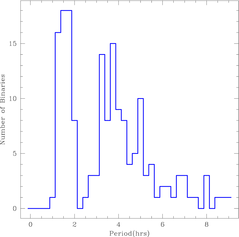
Figure 1: Orbital period distribution of CVs from Clemens, Reid & Gizis(1998).

The origin of the different classes of CVs necessarily involves a detailed consideration of the physics of the accretion disk and its interaction with the stars. This is beyond the scope of the current paper. It is, however, possible to study the existence and origin of the period gap without knowledge of the detailed properties of accretion disks.

A variety of models have been proposed attempting to explain the lack of systems in the period range between 2 and 3 hours (period gap). Almost all of them are different implementations of the suggestion of Robinson et al. (1981) that some mechanism forces secondaries to suddenly shrink when they reach a mass of about 0.3 $M_{\odot}$. Due to the correlation between the mass of the secondary and the orbital period, this happens at about at 3 hours for typical white dwarf masses (see section 3.4). The mass transfer then stops until the secondary touches its Roche lobe again, reestablishing the contact and accretion. Robinson et al. noted that this is the characteristic mass where the secondary becomes fully convective. Theorists have therefore focused on stellar properties that might change at the fully convective boundary.

D’Antona and Mazzitelli (1982) proposed that sudden mixing of ${}^{3}He$ when the star becomes fully convective could cause star to shrink. Later calculations, however, showed that this effect is negligible (McDermott & Taam 1989.) Recent stellar evolution models do not predict any change of mass-radius relation at the point where the star becomes fully convective (see table 1).

Rappaport, Verbunt & Joss (1983) proposed the “disrupted angular momentum loss” model. The most recent description of this model can be found in Howell, Nelson & Rappaport (2000). The timescale for mass accretion is governed by the timescale for angular momentum loss. The Rappaport et al. angular momentum loss timescale for a magnetic stellar wind was shorter than the Kelvin-Helmholtz timescale. The secondary star, being out of thermal equilibrium, could then have a greater radius than a normal main sequence star of the same mass.

Stellar magnetic fields are generated by a dynamo mechanism, and there are plausible theoretical grounds for believing that stellar magnetic field properties could be different in fully convective stars than in stars with radiative cores. As the total stellar mass decreases, the depth of the outer convection zone increases; at very low masses (solar dynamo is thought to be anchored at the interface between the radiative interior and the convective envelope; this mechanism will no longer operate in a fully convective star, which requires a distributed dynamo mechanism (Durney & Latour 1978). McDermot & Taam (1989) claimed that the net effect would be a drastic reduction in angular momentum loss when the secondary became fully convective. With a fully convective secondary, the timescale for angular momentum loss increases dramatically, the secondary shrinks back to its normal radius, and the star is not visible as a CV until gravitational radiation could bring the stars close enough together to cause the secondary to once again overfill its Roche lobe. This model is testable using stellar rotation rates in open clusters with a range of ages and masses.

In this paper, we will show that the empirical timescale for angular momentum loss is much longer that predicted by early models of $\dot{J}$, and that the secondary star will therefore be in thermal equilibrium above and in the period range where the gap is found. Second, the stellar transition between the two dynamo mechanisms appears to be smooth rather than abrupt, suggesting that something other than a phase transition in the angular momentum loss rate must be used to explain the origin of the period gap.

Potential problems with the disrupted magnetic braking model have been discussed in the literature (for example, Clemens et al. 1998 noted the conflict with rotation and activity data in low mass stars.) The assumption that magnetic braking is the only angular momentum loss mechanism for short period CVs also creates some difficulties (Patterson 1998.) Patterson concluded that if the orbital evolution of CVs at low period were driven only by gravitation radiation there would be two serious problems.

First, the predicted period minimum would be at 1.1 hours instead of the observed cutoff at 1.3 hours. Second, the angular momentum loss rates would be very low for short period systems, which implies a low mass accretion rate for the systems near the minimum period. There would then be a large number of CVs observed at or near the minimum period, which is in contradiction with the observations. In order to solve these problems Patterson suggested that there should be some mechanism for destroying CVs before they reach the predicted very high space density. This could be possible if secondaries in CVs lost their thermal equilibrium at about 1.3 hours.

Things become even more interesting with the observational work which have been done in the last decade. Verbunt (1997) re-analyzed the period distribution of cataclysmic variables and came to the conclusion that for Nova Like variables the period gap is not significant. Different classes of variables were found to have considerably different statistical properties. If the period gap does not exist in the intrinsic period distribution of all variables, then models which treat all CVs equally are potentially problematic. Hellier & Taylor (2000) re-examined the distribution of CVs. While they argue against Verbunt’s classification, their work confirms Verbunt’s conclusion that period gap is not significant for Nova-like CVs.

Clemens et al. (1998) proposed an alternate model where the period gap is produced by changes in the mass - radius relation that appear at the edges of the gap. However, this does not address the question of why different types of CVs prefer one or another side of the gap. Kolb, King & Ritter (1998) demonstrated that a sudden change of the mass-radius relationship of the Clemens et al. form would produce two spikes rather than the observed distribution of CVs over period. The question of the impact of the mass-radius relationship on the distribution of CVs is an interesting one that we will return to later.

In this paper we concentrate on the question of the angular momentum loss prescription which is appropriate for CVs. The evolution of CVs is closely related to the angular momentum loss, and therefore it is important to have a correct prescription for it. We introduce an empirical angular momentum loss rate obtained from main sequence stars in open clusters with a range of mass and age. In section 2 we describe the stellar model physics that we use, including a comparison of the empirical angular momentum loss rate to the Rappaport, Verbunt, & Joss (1983) rates which are commonly used in the literature. In section 3 we illustrate a method for inferring the time-averaged mass accretion rate from knowledge of the angular momentum loss rate and the mass-radius relationship. In this section we also infer a mass-period relationship and compare it to the observations. We compare the various timescales of interest for the evolution of CVs and conclude that the secondary star in CV systems should be in thermal equilibrium at and above the 2-3 hour period range. Our results, along with a discussion of the evolutionary state of the secondaries as a possible explanation of the period gap, can be found in section 4.

2 Physics

In this section we describe the physics of CVs relevant to our calculations. The properties of the secondary star are important for understanding the time evolution in CV systems. We describe the global properties of our stellar models in section 2.1. We then briefly describe the angular momentum of the binary system in section 2.2. Section 2.3 is devoted to the important issue of the angular momentum loss prescription for CVs.

2.1 Stellar model

We need the total moment of inertia and radius of the secondary stars in CVs to determine the angular momentum evolution and the mass-radius-period relationship for the system respectively. In addition, the luminosity is required to estimate the Kelvin-Helmholtz timescale.

For the purposes of this paper we constructed a zero-age main sequence set of models to determine the radius, luminosity, and moment of inertia as a function of mass. The angular momentum loss saturation threshold $\omega_{crit}$ (see Section 2.3) as a function of mass was taken from Sills, Pinsonneault & Terndrup (2000). The Yale Rotating Stellar Evolution Code (YREC, Guenther et al. 1992) was used to construct these models. The nuclear reaction rates are taken from Gruzinov & Bahcall (1998). The heavy element mixture is that of Grevesse & Noels (1993), and our models have a metallicity of Z=0.0188. Gravitational settling of helium and heavy elements is not included in these models.

We use OPAL opacities (Iglesias & Rogers 1996) for the interior of the star down to temperatures of $\log T(K)=4$. For lower temperatures, we use the molecular opacities of Alexander & Ferguson (1994). For regions of the star which are hotter than $\log T(K)\geq 6$, we used the OPAL equation of state (Rogers, Swenson & Iglesias 1996). For regions where $\log T(K)\leq 5.5$, we used the equation of state from Saumon, Chabrier & Van Horn (1995), which calculates particle densities for hydrogen and helium including partial dissociation and ionization by both pressure and temperature. In the transition region between these two temperatures, both formulations are weighted with a ramp function and averaged. The equation of state includes both radiation pressure and electron degeneracy pressure. For the surface boundary condition, we used the stellar atmosphere models of Allard & Hauschildt (1995), which include molecular effects and are therefore relevant for low mass stars. We used the standard Böhm-Vitense mixing length theory (Cox & Guili 1968; Böhm-Vitense 1958) with $\alpha$=1.72. This value of $\alpha$, as well as the solar helium abundance, $Y_{\odot}=0.273$, was obtained by calibrating models against observations of the solar radius ($6.9598\times 10^{10}$ cm) and luminosity ($3.8515\times 10^{33}$ erg/s) at the present age of the Sun (4.57 Gyr).

The zero-age main sequence model properties define the normal single star mass-moment of inertia, mass-radius, and mass-luminosity relationships that we will apply to the study of CVs.

m r l I[cgs] $\omega_{crit}$ 0.1 0.118 0.001 2.81e+51 9.50e-7 0.2 0.216 0.005 1.89e+52 2.31e-6 0.3 0.289 0.011 5.04e+52 3.69e-6 0.4 0.361 0.019 9.80e+52 5.13e-6 0.5 0.451 0.037 1.61e+53 6.76e-6 0.6 0.553 0.074 2.38e+53 1.16e-5 0.7 0.643 0.146 3.21e+53 1.45e-5 0.8 0.711 0.266 4.16e+53 1.82e-5 0.9 0.785 0.444 5.36e+53 2.27e-5 1.0 0.883 0.690 6.85e+53 3.00e-5 1.1 0.995 1.028 8.61e+53 4.39e-5 1.2 1.119 1.476 1.06e+54 8.66e-5

Table 1 gives the radius and luminosity in solar units and the cgs moment of inertia as a function of the mass in solar masses. The important saturation threshold $\omega_{crit}$ is discussed in section 2.3. We interpolate in the above table to get stellar properties as a function of mass. Some investigators use linear or power-law fits for these global properties. The mass-radius relationship for unevolved secondary stars can be expressed as $r\approx 0.901m+0.014$. The mass-luminosity relationship can be fit by a broken power law of the form $\lg{(l)}\approx 2.022\lg{(m)}-0.878,m\leq 0.5;4.730\lg{(m)}-0.117,m\geq 0.5$. Finally, the moment of inertia as function of mass is described by $\lg{I}\approx 2.397\lg{m}+53.91$.

2.2 Angular momentum

The timescale for tidal synchronization is much shorter than the characteristic evolutionary timescale for the orbital period range of cataclysmic variables (see section 3.) We can therefore assume that the rotation periods of the stars and the system are the same; because of the small moment of inertia of the white dwarf its rotational angular momentum can be safely neglected. Helioseismic data for the Sun indicates that the rotation rate in the surface convection zone is independent of radius (e.g. Schou et al. 1998) Most helioseismic inversions indicate that the rotation in the solar core is similar to that of the surface convection zone down to a depth of order 0.2 solar radii (Chaplin et al 1999); there is some debate about the situation in deeper layers (compare Chaplin et al. 1999 with Gavryuseva, Gavryusev, & di Mauro, 2000) The stars in CV systems rotate relatively rapidly (implying a short timescale for internal angular momentum transport) and have deep surface convection zones, so it is therefore reasonable to assume solid-body rotation in the secondary star.

The total angular momentum of the system can thus be written in the form :

$$J=M_{\odot}^{5/3}G^{2/3}m_{1}m_{2}m^{-1/3}\omega^{-1/3}+I(m_{2})\omega$$ (1)

where $m_{1}$ and $m_{2}$ are the masses of the primary and secondary, $m$ is the total mass of the system, $\omega$ is the angular rotation velocity of the secondary, and $I(m_{2})$ is the moment of inertia of the secondary star. The first term describes the orbital angular momentum of the system, and the second term is the spin angular momentum of the secondary star.

2.3 Angular momentum loss

The evolution of a CV is determined by the masses of the primary and secondary, the structural properties of the secondary star, and the angular momentum loss rate. We will show in section 3.5 that the mass loss rate can be inferred from the mass-radius relationship and knowledge of the angular momentum loss rate under the assumption of marginal contact. The angular momentum loss prescription is therefore a crucial ingredient for the study of CVs.

There are two general mechanisms for the transferring angular momentum out of the system.

First, binary systems emit gravitational radiation, which carries away angular momentum. The rate of angular momentum loss increases as the orbital separation decreases, but it decreases as the total mass of the system decreases. Because both the secondary mass and the orbital separation decrease as CV systems evolve, the net effect is a loss mechanism that does not depend strongly on the orbital period.

We use the following expression for the angular momentum loss from gravitational radiation (see, for example, Landau & Lifshitz 1939):

$$\left(\frac{dJ}{dt}\right)_{grav}=-\frac{32}{5}\frac{G^{7/2}}{c^{5}}a^{-7/2}m_{1}^{2}m_{2}^{2}\sqrt{m}M_{\odot}^{5/2}$$ (2)

Where $m_{1}$ , $m_{2}$ , $m$ are the white dwarf mass, secondary mass, and total mass respectively; $a$ is the separation between the stars, which can be obtained from Newtons’ form of Kepler’s third law $a=\left(\frac{GmM_{\odot}}{\omega^{2}}\right)^{\frac{1}{3}}$.

However, gravitational radiation alone cannot explain the orbital evolution of low mass stars (e.g. Patterson 1984, Rappaport, Verbunt & Joss 1983.) Secondary stars with sufficiently deep surface convection zones experience angular momentum loss from a magnetic stellar wind. Because binaries at the orbital periods of CVs are tidally synchronized (Patterson 1984), angular momentum lost from the secondary star is removed from the orbital angular momentum and the orbital separation of the binary system is reduced. Weber & Davis (1967) predicted an angular momentum loss rate proportional to $\omega^{3}$ based upon a study of the solar wind; this is consistent with the time dependence of rotation inferred from early studies of solar-type stars in open clusters (Skumanich 1972). The strong dependence of the angular momentum loss rate on the angular velocity results primarily from scaling the mean magnetic field strength to the rotation rate. Rappaport, Verbunt &Joss (1983) developed an empirical prescription that is commonly used in studies of CVs; their relationship is given by:

$$\left(\frac{dJ}{dt}\right)_{wind}\approx-3.8\cdot 10^{-30}\cdot M_{\odot}R_{\odot}^{4}\cdot mr^{\gamma}\omega^{3}\,dyn\,cm.$$ (3)

where $\gamma$ is a dimensionless parameter in the range from 0 to 4.

There are serious difficulties with applying any angular momentum loss model which scales as $\omega^{3}$ to observations of young low mass stars. The spindown of rapid rotators is predicted to be extremely fast (see for example Pinsonneault, Kawaler, & Demarque 1990), but rapidly rotating low mass stars are observed in young open clusters (Stauffer & Hartmann 1988). Both chromospheric activity indicators and X-ray studies, furthermore, can be used as proxies for measurements of the strength of stellar magnetic fields. There is now extensive empirical evidence that both chromospheric and coronal indicators become independent of the rotation rate above a mass-dependent critical angular velocity (e.g. Patten & Simon 1996); this would imply a much lower angular momentum loss rate for rapid rotators. We note that this does not contradict the overall Weber & Davis (1967) model in the case of slow rotators; however all of the direct and indirect observational tests in low mass stars and open clusters of different ages indicates that it overestimates the angular momentum loss rate for rotation periods shorter than 2.5 - 5 days.

A number of different theoretical groups have investigated the spindown of low mass stars (Queloz et al. 1998; Collier-Cameron & Jianke 1994; Keppens, MacGregor, & Charbonneau, 1995; Krishnamurthi et al. 1997; Sills, Pinsonneault, & Terndrup, 2000). In all cases the survival of rapid rotation in young open clusters required a modification of the angular momentum loss law at high rotation rates. We therefore use an angular momentum loss prescription with the same function form as that of Sills, Pinsonneault, & Terndrup (2000):

$$\left(\frac{dJ}{dt}\right)_{wind}=-K_{w}\cdot\sqrt{\frac{r}{m}}\cdot\left\{\begin{array}[]{ll}\omega^{3}&{\rm for}\;\omega\leq\omega_{crit}\\ \omega\omega^{2}_{crit}&{\rm for}\;\omega>\omega_{crit}\end{array}\right.$$ (4)

Here $\omega_{crit}$ is the critical angular frequency at which the angular momentum loss rate enters into the saturated regime. The constant $K_{w}\approx 2.7\cdot 10^{47}\,g\,cm\,s$ and is calibrated to reproduce the known solar rotation period at the age of the Sun (see Kawaler 1988 for a discussion of the ingredients and uncertainties.) The value of $\omega_{crit}$ can be inferred empirically by reproducing the observed spindown of low mass stars as a function of mass and age. There is therefore one clear implication from the large database of observational and theoretical work in the study of rotation in low mass open cluster stars: angular momentum loss prescriptions of the form used by Rappaport, Verbunt & Joss (1983) greatly overestimate angular momentum loss rates for secondary stars in the period range of interest for the study of CVs. Solokani, Motamen & Keppens (1997) propose an alternate physical mechanism (concentration of magnetic fields close to the pole for rapid rotators), but their model predicts a very similar angular momentum loss rate to the saturated wind model.

The second important result in the context of CV studies is the observed mass dependence of the angular momentum loss rate. It has long been known that the observed saturation threshold for chromospheric and coronal activity indicators is mass dependent (see Noyes et al. 1984; Patten & Simon 1996). Krishnamurthi et al. (1997) found that a scaling of $\omega_{crit}$ with the inverse Rossby number (the ratio of the rotation period to the convective overturn timescale) gave a reasonable fit to the observed timescale for spindown as a function of mass from 0.6 - 1.2 solar masses. Similar Rossby number scalings are also found to describe the saturation of activity indicators (Krishnamurthi et al. 1998) and are expected on general theoretical grounds for a shell dynamo (e.g. Durney & Latour 1978). In other words, the timescale for stars to spin down increases as the mass decreases.

Observations of both activity indicators and rotation velocities down to very low masses have been obtained in open clusters with a range of ages (Jones, Fischer, & Stauffer 1996; Stauffer et al. 1997; Terndrup et al. 2000; Reid & Mahoney 2000). There is no observational support for an abrupt change in angular momentum loss properties at the point where stars become fully convective (around 0.3 solar masses.) Sills, Pinsonneault, & Terndrup (2000) found that the mass dependence of $\omega_{crit}$ could no longer be fit by a Rossby scaling below 0.5 solar masses; this suggests that the transition from a shell to a distributed dynamo occurs well above the fully convective boundary. However, some angular momentum loss was needed even below the fully convective boundary in order to explain the observed spindown of Hyades stars relative to Pleiades stars. Hawley (1999) and Hawley et al. (1999) also found that the timescale for high activity levels to survive was a smooth function of mass.

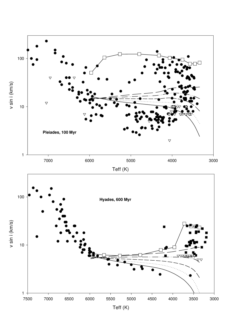
Figure 2: Theoretical models for the upper envelope of rotation compared with data in the Pleiades (top) and Hyades (bottom). The solid line with the open boxes is the empirical model (0.2 - 1.1 $M_{\odot}$ in the 0.1 $M_{\odot}$ increments). The group of lines below are the RVJ models with $\gamma=0,1,2,3,4$. Pleiades data is taken from Terndrup et al. 2000, Stauffer et al. 1997, and Anderson et al. 1966. Hyades data is taken from Radick et al. 1987, Terndrup et al. 2001, and Kraft 1965.

We compare the predicted stellar rotation rates using the Sills, Pinsonneault, & Terndrup (2000) empirical angular momentum loss law as a function of mass and the Rappaport, Verbunt, & Joss (1983) angular momentum loss law with Pleiades and Hyades data in Figure 2. For these models we chose an initial rotation period at the deuterium-burning birthline of 10 days (corresponding to the average rotation period inferred for T Tauri stars from Choi & Herbst 1996). Because of the strong feedback in the unsaturated angular momentum loss law, choosing a much shorter initial rotation period would yield very similar results for the Rappaport et al. loss rates. This choice of initial conditions corresponds to the expected upper envelope of rotation rates that are observed in open clusters.

We note that because the most rapid rotators are rare (roughly 3% of the total population) the upper envelope as a function of effective temperature is subject to Poisson noise. However, the existence of stars rotating more rapidly than 10 km/s in the Pleiades is a direct contradiction of the predictions of an unsaturated angular momentum loss law. We do see evidence of a transition away from a pure Rossby scaling of the saturation threshold in the coolest Hyades stars. The upturn in rotation at the low mass end indicates a change in the efficiency of angular momentum loss (a pure Rossby scaling would reduce to the older angular momentum loss rates at this age.) However, this transition occurs at 0.6 solar masses, well above the fully convective boundary. Furthermore, there is clear evidence for spindown even in the lowest mass stars for which we have data. This extends into the very low mass regime from field star data (Hawley et al. 1999.)

We compare our empirical angular momentum loss rates as a function of secondary mass with that from the Rappaport et al.(1983) prescription in Figure 3; in the latter prescription magnetic braking is stopped at 0.3 solar masses and the only angular momentum loss mechanism for the low mass stars is gravitational radiation. The older angular momentum loss rate is overestimated by about 2 orders of magnitude at the period gap.

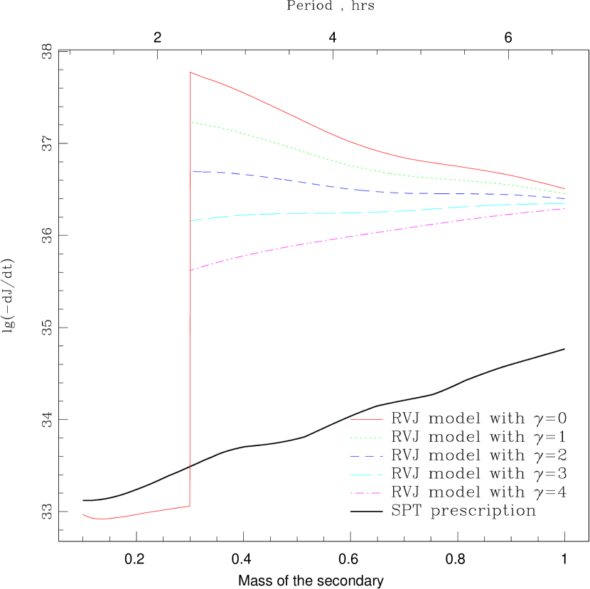
Figure 3: Angular momentum loss for a system with mass-conserving primary of 0.62$M_{\odot}$. Dashed lines are Rappaport,Verbunt&Joss model, thick solid line is Sills, Pinsonneault & Terndrup (2000) prescription.

We note that the stellar data becomes sparse below about 0.2 solar masses, and further observational data on very low mass stars would be useful to constrain the empirical angular momentum loss law at the bottom of the main sequence. It is also possible that for the faintest stars the timescale for angular momentum loss could become much longer (see Basri & Marcy 1995 for a discussion of this point.) Any such effect, however, occurs at a significantly lower mass than the fully convective boundary and therefore has no direct effect on the existence of the period gap. This change in the angular momentum loss law has important consequences for the predicted time evolution of CVs which we present in the next section.

3 Model, limitations and solution.

This section describes our model for the evolution of CVs. Section 3.1 describes our mass-radius relation, which is one of the most important ingredients in the evolution of cataclysmic variables. We summarize all of the equations and assumptions in our models in Section 3.2. Section 3.3 gives a motivation for the assumption of marginal contact. We compares our inferred theoretical mass-period relation to the empirical one in section 3.4, and discuss the time-averaged mass accretion rate as a function of period in section 3.5. Section 3.6 is devoted to a comparison of the timescales of different processes.

3.1 Mass - radius relation for the secondary

In this work we begin with the theoretical mass-radius relationship for single unevolved low mass main sequence stars described in section 2. These models provide a natural starting point for the study of CVs; if the secondary star begins with a mass at or lower than $\sim$0.8 solar masses then there will be little nuclear evolution within a Hubble time and such objects would therefore be expected to follow the unevolved mass-radius relationship. In principle, both the rapid rotation of CV secondaries and the tidal gravitational field of the white dwarf primary could affect the mass-radius relationship. However, Kolb & Baraffe (1999) investigated the impact of rotation and tidal distortion on the properties of CV secondaries. They concluded that these effects are small even in short period CVs. We therefore do not include the structural effects of rotation and tidal deformation in our models. We do note, however, that if the secondary star is not chemically homogeneous then meridional circulation and rotational instabilities could induce significant mixing; as we will see below, there is possible evidence that some CV secondaries could have experienced significant nuclear evolution on the main sequence. We defer a treatment of these effects to a paper in preparation.

The secondary star in CVs could also be partially evolved. This could occur if the secondary and primary stars had similar mass; alternately, if the timescale for CV evolution was sufficiently long, primary stars more massive than $\sim 1$ solar mass could experience significant nuclear burning during the CV phase. A proper treatment of this effect would require calculation of a range of initial secondary masses and evolutionary states and stellar interiors models which evolve under the presence of mass loss; we are constructing such models in a paper in preparation. We have also considered two simplified models which do not begin in a chemically homogeneous state to test for the impact of the evolutionary state of the primary on the mass-radius relationship. We evolved 1.0 and 1.2 solar mass, solar composition models until they overflowed their Roche lobes at an initial orbital period of 10 hours for an assumed primary white dwarf mass of 0.6 solar masses. We then removed mass from them without further nuclear burning; these models are systematically larger at a given mass than the chemically unevolved models until they become fully mixed at low total stellar mass.

3.2 Model and limitations

Our system of equations is:

$$\left\{\begin{array}[]{l}J=M_{\odot}^{5/3}G^{2/3}m_{1}m_{2}m^{-1/3}\omega^{-1/3}+I(m_{2})\omega\\ \frac{dJ}{dt}=\left(\frac{dJ}{dt}\right)_{w}+\left(\frac{dJ}{dt}\right)_{g}\\ r_{2}=f(m_{2})\end{array}\right.$$ (5)

When the mass of the secondary drops below $\sim 0.07M_{\odot}$ the radius increases with decreased mass (see for instance Burrows et al. 1993). This would result in increased period for decreased mass; systems which pass this critical point are sometimes called period bouncers in the literature. We do not consider secondaries with masses below this limit.

Accretion happens only when the secondary star overfills its Roche lobe. In order to take this into account we introduce a dimensionless parameter $y$ which is defined as the ratio of the star’s radius to the Roche distance from the center of the secondary. For the Roche distance from the secondary we use the relation derived by Eggleton (1983):

$$y=\frac{R}{R_{L}}=\frac{R_{\odot}r_{2}}{a}\cdot\frac{0.6\left(\frac{m_{2}}{m_{1}}\right)^{2/3}+\ln{\left[1+\left(\frac{m_{2}}{m_{1}}\right)^{1/3}\right]}}{0.49\left(\frac{m_{2}}{m_{1}}\right)^{2/3}}$$ (6)

Accretion only occurs if $y\geq 1$. In the marginal contact assumption described below, we constrain $y$ to be unity.

3.3 Marginal contact

The usual way to make the system of equations (10) closed is to add a prescription for the mass accretion rate (D’Antona et al 1989, Hameury 1991). This is obtained indirectly from observations (see Patterson 1984, Rutten, Paradijs and Tinbergen 1992), or from semi-analytic expressions (D’Antona et al 1989). The uncertainties in the observed mass loss rates are significant; the estimates of mass accretion are based on poorly understood physics of accretion disks and the distances to CVs are not well constrained (Patterson 1984, Rutten et al 1991).

Directly using the inferred mass loss rates leads to oscillations of the period in a small timescale (Hameury 1991). Due to orbital angular momentum loss, the period of the system decays until the secondary overfills its Roche lobe and mass loss sets in. When mass is lost from the system the moment of inertia is reduced, which causes the orbital period to increase. If the timescale for mass accretion is short enough this can drive the system out of contact and lead to oscillations in the orbital period. To resolve this instability some investigators have introduced a dependence of the mass accretion rate on the extent to which the Roche lobe is overfilled (Hameury 1991, D’Antona et al. 1989).

However, we contend that knowledge of the angular momentum loss rate and the mass-radius relationship specifies the time-averaged mass loss rate with a small uncertainty. CV systems will tend to remain close to marginal contact; a small decrease in orbital period will drastically increase the mass loss rate and drive the stars apart because of the decrease in moment of inertia, while an increase in orbital period will drive $y$ below unity and detach the stars, causing the stars to come closer from angular momentum loss. For any given primary and secondary masses, this implies that the orbital period should be close to the case where $y$ is unity. If the mass-radius relationship is known, this can be directly converted into a mass-orbital period relationship. There is also a similar and well constrained relationship between the total angular momentum and the orbital period.

There is no strong motivation for the existence of changes of mass accretion in a small timescale. But even if such oscillations exist, they would not make difference in time averaged angular momentum loss rate. First, such oscillations would be of order of the timescale for the accretion disk, which is much lower than any other characteristic time for CVs. Secondly, the weaker dependence of the saturated angular momentum loss rate upon $\omega$ than in the older $\dot{J}$ prescriptions would imply a smaller amplitude of fluctuations of angular momentum loss. Therefore, when averaged over a time larger than the characteristic time for the accretion disk, the angular momentum rate would not be very sensitive to such oscillations.

We therefore introduce the assumption of marginal contact; namely that the secondary is always at the critical orbital period where it begins to overflow its Roche lobe ($y=1$). The time-averaged mass accretion rate is inferred from the angular momentum loss rate and the mass-radius relationship. This can be regarded as a steady-state accretion rate. It is mathematically stable; of course, this does not guarantee the physical stability of such a flow in a real accretion disk. For understanding the period distribution of CVs, however, this should be a good approximation. A comparison of the steady-state mass loss rate to the observed one, and its implications, are discussed in section 3.6.

The mass-radius relationship that we use is for secondary stars in thermal equilibrium; this assumption can be tested in two different ways. In the next section we compare our mass-period relationship for both unevolved and evolved secondary stars to the observed one; in section 3.5 we compare the Kelvin-Helmholtz timescale to the timescales for angular momentum and mass loss.

3.4 The Secondary Mass-Orbital Period Relationship

The mass-period relation for the secondary can be obtained in the assumption of marginal contact with one final ingredient: the amount of mass from the secondary that the primary retains. The rates of change of the primary and secondary masses are related by

$$\frac{dm_{1}}{dt}=-\chi\frac{dm_{2}}{dt}$$ (7)

where $\chi$ is a dimensionless parameter that varies from 0 to 1. In the case of $\chi=1$ the system conserves its total mass. In the case of $\chi=0$ the primary mass is constant and the rest of the mass is lost in nova outbursts.

If one specifies the masses and the value of $\chi$, for a given mass-radius relation and angular momentum loss rate, the period is defined. This yields a relationship between the mass of the secondary and period for CVs. The rate of period change is correlated with the mass accretion rate through the mass of the secondary-period relation:

$$\frac{d\omega}{dt}=\left.\dot{m_{2}}\frac{d\omega}{dm_{2}}\right|_{m_{2}+\chi m_{1}=const}$$ (8)

By requiring $y=1$ we obtain the relation:

$$R_{\odot}r_{2}(m_{2})=\left(\frac{G(m_{1}+m_{2})M_{\odot}}{\omega^{2}}\right)^{\frac{1}{3}}\cdot\frac{0.49\left(\frac{m_{2}}{m_{1}}\right)^{2/3}}{0.6\left(\frac{m_{2}}{m_{1}}\right)^{2/3}+\ln{\left[1+\left(\frac{m_{2}}{m_{1}}\right)^{1/3}\right]}}$$ (9)

The mass-period relation is shown in figure 4 together with two empirical fits $m_{2}=(0.038\pm 0.003)P^{1.58\pm 0.09};m_{2}=(0.126\pm 0.011)P-(0.11\pm 0.04)$ taken from recent work on CV secondaries by Smith and Dhillon (1999).

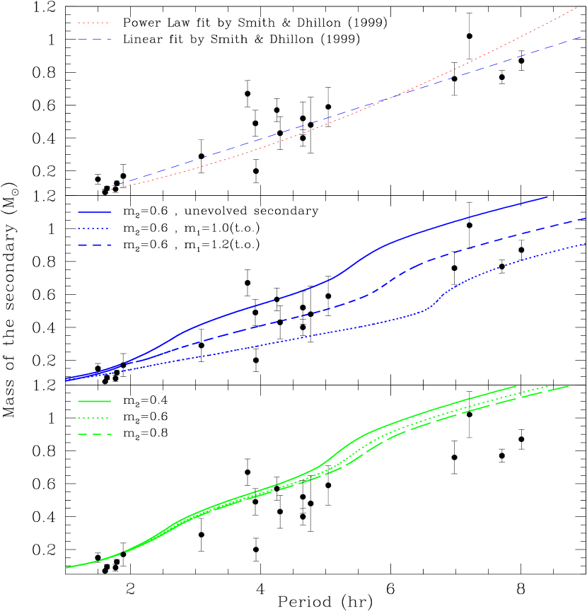
Figure 4: The mass of the secondary - period relation.

In the top panel we show the data and empirical fits. The bottom panel illustrates the effect of changing the primary mass in the range of 0.4 to 0.8 solar masses; this has only a small impact on the predicted mass-period relationship. In the middle panel we compare our unevolved secondary models and two simplified evolved secondary models with the data.

The unevolved relationship is a good match to the upper envelope of the data. Especially at longer periods, there is a tendency for some of the data to lie at lower mass for a fixed period, which indicates a larger radius than predicted by the unevolved models. However, the observed range of mass-period relationships is consistent with the range spanned by our partially evolved and unevolved models.

At short periods, the M-R relationship for our evolved models could be altered because there is significant helium enrichment and we are using model atmospheres with a solar mix. Even though the predictions are close to the data around periods of two hours, the error bars there are smaller. This could also indicate that non-spherical effects become important at low period, which is plausible as those stars could be severely distorted by their much more massive and close WD companion.

In conclusion, the models are consistent with the data if a range of secondary evolutionary states are considered. There is evidence for a departure from thermal balance only if the unevolved models are considered as the only ones. We directly compare the relevant timescales in the next section. We also compare the data with the inferred mass loss rates for different mass-radius relationships in the section that follows. We contend that these diagnostics are more consistent with a range of evolutionary states rather than a departure from thermal balance.

3.5 Timescales

The governing timescale for the orbital evolution of CVs is the timescale for angular momentum loss. Our mass-radius relationship assumes models in thermal equilibrium, so it is important to compare the timescales for orbital change and for secondaries to establish thermal balance (e.g. the Kelvin-Helmholtz timescale.) In addition, we can infer the steady-state accretion rate and the timescale for mass loss from the secondary.

For angular momentum loss, mass accretion and period change timescales can be estimated by $\tau_{X}=\left|\frac{X}{\dot{X}}\right|$ where $\dot{X}$ is the time derivative of variable $X$.

The steady-state mass loss rate can be derived as follows. Taking the derivative from the angular momentum equation (1) and using equation (8), one can get :

$$\begin{array}[]{l}\dot{J}=\dot{m_{2}}\left(A\omega^{-1/3}m^{-1/3}(m_{1}-\chi m_{2})-\frac{1}{3}Am_{1}m_{2}m^{-4/3}\omega^{-1/3}(1-\chi)\right.\\ -\frac{1}{3}Am_{1}m_{2}m^{-1/3}\omega^{-4/3}\frac{d\omega}{dm_{2}}+\left.I(m_{2})\frac{d\omega}{dm_{2}}+\omega\frac{dI}{dm_{2}}\right)\end{array}$$ (10)

We can now solve for $\dot{m_{2}}$ because we know the angular momentum loss rate, moment of inertia as a function of mass and the mass-period relationship, which gives $\frac{d\omega}{dm_{2}}$:

$$\begin{array}[]{l}\dot{m_{2}}=\dot{J}\left(A\omega^{-1/3}m^{-1/3}(m_{1}-\chi m_{2})-\frac{1}{3}Am_{1}m_{2}m^{-4/3}\omega^{-1/3}(1-\chi)\right.\\ -\frac{1}{3}Am_{1}m_{2}m^{-1/3}\omega^{-4/3}\frac{d\omega}{dm_{2}}\left.+I(m_{2})\frac{d\omega}{dm_{2}}+\omega\frac{dI}{dm_{2}}\right)^{-1}\end{array}$$ (11)

This defines the steady-state mass accretion rate directly, and the rate of change of angular frequency through equation (7). We solve this set of equations iteratively.

For CVs the timescale for tidal synchronization is very short, of order $5000$ years (Warner 1995); this timescale is much shorter than the other relevant ones for the system. The thermal relaxation or Kelvin - Helmholtz timescale for the secondary is

$$\tau_{KH}\approx\frac{3}{4}\frac{GM^{2}}{LR}$$

We use the mass-radius and mass-luminosity relationships described earlier. The relevant timescales for cataclysmic variables are illustrated in figure 5.

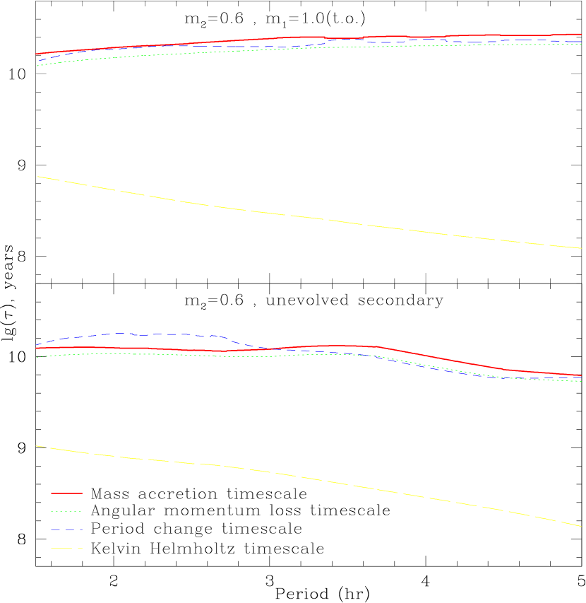
Figure 5: Comparison of timescales.

The timescales for mass accretion and period change are comparable and follow the timescale for angular momentum loss, because in the assumption of marginal contact they are both defined by it. The Kelvin-Helmholtz timescale is shorter; therefore we can infer that the secondary stars in CVs should be in thermal equilibrium at all periods. We also note that the timescales for the evolution of CVs are much longer than in previous studies, which will have a profound impact. It is no longer correct to assume that the timescale for CVs to reach the period gap is less than a Hubble time. Rather than treating the period distribution of CVs as being in a steady-state, this implies that finite age effects could be crucial.

Our timescale estimates imply that the secondary stars are in thermal equilibrium which is consistent with unperturbed mass-radius relationships that we have used. This is in contrast with the results from earlier loss laws, and it is a straightforward consequence of our angular momentum loss prescription. Early prescriptions for angular momentum loss predicted much higher loss rates for rapid rotators than are consistent with modern open cluster data. A relatively low angular momentum loss of the form we advocate leads to a low mass accretion rate and a longer evolutionary timescale. In addition, the open cluster data indicate that angular momentum loss works even for stars below the fully convective boundary.

This supports the idea that a range of evolutionary states, rather than a departure from thermal balance, is responsible for the stars with low mass at fixed period discussed in the previous section. In a recent paper Rubenstein(2001) demonstrated that evolutionary stage and metallicity are able to explain the observed Period-Color relation for contact binaries. Our results are consistent with this work, although we are describing the mass - period relationship. The closer correspondence between the observed properties of CVs and evolved stellar models has been noted earlier (e.g. Patterson 1984; Baraffe & Kolb 2000).

3.6 Comparison of Mass Accretion Rates

In this section we compare our mass accretion rates to the data. We begin by noting that the uncertainties in the empirically derived mass accretion rates are significant (Patterson 1984). First, it can be difficult to infer the luminosity. The distances to CVs are not well constrained. The bolometric correction is based upon the properties of x-ray emitting systems and involves the complex physics of accretion disks. Knowledge of the luminosities of CV systems is therefore non-trivial.

Accretion rates are derived from the luminosity via the expression $L_{bol}=kGM_{1}\dot{M}/R_{*}$ (Patterson 1984) which involves an additional unknown: the parameter $k$ is efficiency of conversion of gravitational energy to radiation. Patterson is using the low spatial abundance of CVs as one of the arguments justifying high mass accretion rate. With a high mass accretion rate, CV systems will die rapidly. However, we suggest that the solution for the slow spatial abundance of CVs is actually slow angular momentum evolution. Systems with relatively high orbital periods after the common envelope phase ($\sim$3-5 days) would not come into contact and hence most of them exist as planetary nebulae with a companion, rather than CVs.

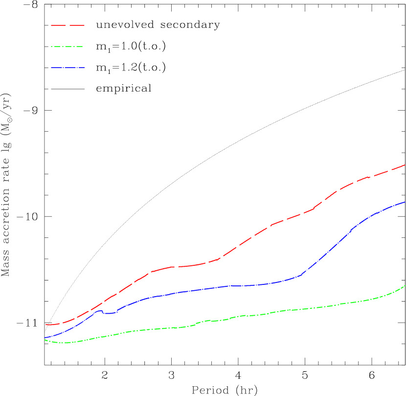
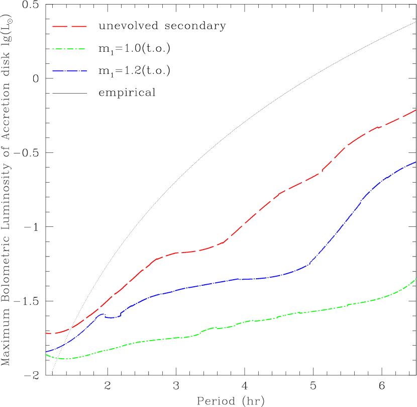
Figure 6: Comparison of the time averaged mass accretion rate and maximum possible accretion disk luminosity for our 3 models. The thin solid line is the empirical fit from Patterson (1984).

The theoretical mass accretion rate is derived using formula (10) assuming the maximum possible theoretical luminosity of the accretion disk ($k=1$). We compare the mass loss rates inferred from both the unevolved and evolved M-R relationships to the empirical results by Patterson (1984) in figure 6. The inferred observed rates are closer to the evolved than unevolved models, but the empirical results are systematically significantly higher than the theoretical predictions in both cases. There are three possible classes of explanations. First, this could reflect systematic errors in the measured rates. Alternately, this could indicate a problem with the mass-radius relationship; as in the case of the mass-period relationship we find that evolved secondaries provide a better fit to the data. Finally, there is an difference between the instantaneous mass loss rate that is observed and the time-averaged mass loss rate obtained under marginal contact. This discrepancy could therefore reflect a duty cycle, where the systems are only in contact (and visible as CVs) for a fraction of their total lifetime. With better distance estimates and new x-ray satellites it will be possible to distinguish between these different explanations.

4 Summary

The most important result of this paper comes from applying the empirical angular momentum loss rates inferred from young single stars to the evolution of cataclysmic variables. In contrast to some popular models, we find that the timescale for angular momentum loss from CV secondaries is significantly longer than previously assumed. This has two direct and important consequences.

First, the angular momentum loss timescale is significantly longer than the Kelvin-Helmholtz timescale for all but the shortest period CVs, which implies that these objects are in thermal balance and not dramatically increased in radius relative to normal single stars. Second, the timescale for CV evolution is increased significantly. The distribution of CVs as a function of orbital period has traditionally been treated under the assumption that the time for a CV to cross from long period to the period gap was much shorter than a Hubble time because the timescale for angular momentum loss was small. For unevolved secondaries, we find that the evolutionary timescale to reach the period gap can approach the Hubble time; this raises the intriguing possibility that finite age effects could be significant for understanding the period distribution of CVs.

Furthermore, there does not appear to be a discontinuity in angular momentum loss properties at the onset of the fully convective boundary. We believe that there are a number of independent lines of evidence that support this claim; the strongest and most direct is the absence of an abrupt change in the surface rotation velocities as a function of age at the relevant mass in open clusters.

We note that including angular momentum loss from secondary stars also improves the agreement between observation and theory for the shortest period CVs (1.3 hr vs 1.1 hr); the empirical angular momentum loss rate that we infer (1.5 times gravitational radiation) is at the level Patterson (1998) found was needed to produce the observed minimum CV period.

Therefore, something other than the angular momentum loss rates must be responsible for the existence of the CV period gap. One intriguing possibility is that the presence of two distinct peaks in the distribution of CVs could reflect two distinct populations of objects with different origins. This is made more likely by the long timescale for angular momentum loss. The evolutionary state of the secondary at the onset of the CV phase and the physics of the common envelope phase present two potential culprits.

If the primary and secondary have similar mass, the secondary could be significantly evolved and would therefore obey a different mass-radius relationship than an unevolved secondary. A star that is near hydrogen core exhaustion will be systematically larger than an unevolved star of the same total mass. Because the angular momentum loss timescale is long, there may also be significant nuclear evolution during the CV phase even for unevolved secondaries that begin at masses of order 1 solar mass or higher. There are a number of long period CVs with radii larger than those inferred from the unevolved mass-radius relationship, which provides some support for the idea that some CV secondaries may be of this type.

Another possible mechanism for producing evolved secondary stars is related to the physics of the common envelope phase. The most powerful argument against a large fraction of evolved secondaries has been the shape of the IMF, which would predict many more low mass companions. However, we note that the angular momentum loss rate will also have strong consequences during the common envelope phase of evolution. Models for common envelope evolution (de Kool 1990; Iben & Livio, 1993; Yungelson et al. 1993) show that common envelope systems with a white dwarf and a main sequence secondary result in binaries with initial periods significantly longer than CVs: typically more than $\sim$ 3 days). The period evolution for such binaries is very slow with the empirical angular momentum loss rate. This is especially true for lower mass secondaries that will have lower loss rates. The timescale for the formation of CVs can be longer than age of the Galaxy. Only systems with very short orbital periods will go into contact in a Hubble time (less than $\sim$ 2-5 days, with the lower bound applicable for the lowest mass stars while the upper bound is applicable for the highest mass stars). Because the nuclear timescale for stars above a solar mass can be less than the timescale for common envelope products to spiral together, this would create a selection effect favoring evolved higher mass secondary stars as the companions to CVs. Prior to the CV phase the secondary star is evolving, and once it get into contact, it has a higher radius than a ZAMS star of the same mass. This radius remains systematically higher until the secondary becomes fully convective. This explains 2 things simultaneously: the better fit to observational data by evolved stars and the low space density of CVs (see Patterson 1984, 1998). To state things another way, CVs are both longer-lived and more difficult to produce in the presence of mild angular momentum loss. There would be some low mass secondaries that, by chance, were born with short enough periods to cross the period gap. We stress that there is no a priori reason for all CV secondaries to be evolved, but rather that some may be and that this could produce two different populations with different period distributions.

Another effect that may prove important in this context is the behavior of chemically evolved stars as they approach the fully convective boundary. Once evolved secondaries reach the fully convective phase they would become fully mixed and move close to the unevolved mass-radius relationship. This would correspond to a significant change in radius over a small range in age, which would in turn correspond to a small mass loss rate and a relatively long evolutionary timescale at this critical point. In this scenario, the peak in the CV distribution at 3 hours would correspond to a population of mostly evolved secondaries. We note that meridional circulation mixing of such evolved stars could also cause a transition to a chemically homogeneous state at short period; we intend to explore models of this type. In the two simple trial models of this type that we ran, the transition to a fully convective state actually occurred at a range of periods; however, we neglected meridional mixing and nuclear evolution during the CV phase.

Finally, the time-averaged mass loss rate from the assumption of marginal contact is significantly less than the claimed observational rates. This could imply that CVs have a short duty cycle. However , we believe that the observational uncertainties in the empirical mass loss rates should be carefully examined before drawing strong conclusiond of this type.

5 Acknowledgment

M.P. would like to thank P. Eggleton and Mark Wagner for useful discussions.

References

- (1) Alexander, D. R., & Ferguson, J. W. 1994, ApJ, 437, 879.
- (2) Allard, F., & Hauschildt, P. H. 1995, ApJ, 445, 433.
- (3) Anderson, C.M., Stoeckly, R. & Kraft, R.R. 1966, ApJ, 143, 299.
- (4) Baraffe, I., Chabrier, G., Allard, F., & Hauschildt P.H. 1998, A&A, 337, 403.
- (5) Baraffe, I., Kolb, U. 2000, MNRAS, 318, 354.
- (6) Basri, G. 1987, ApJ, 316, 377.
- (7) Basri, G. & Marcy, G.W. 1995 AJ 109, 762.
- (8) Beuermann, K., Baraffe, I., Kolb, U., & Weichhold, M. 1998, A&AS, 339, 518.
- (9) Böhm-Vitense, E. 1958, Zs. f. Ap., 46, 108.
- (10) Burrows, A., Marley, M., Hubbard, W. B., Lunine, J. I., Guillot, T., Saumon, D., Freedman, R., Sudarsky, D., Sharp, C. 1997, ApJ, 491, 856.
- (11) Burrows, A., Hubbard, W. B., Saumon, D., & Lunine J. I. 1993, ApJ, 406, 158.
- (12) Chaplin, W.J. et al 1999, MNRAS, 308, 405.
- (13) Choi, P.I. & Herbst, W. 1996, AJ, 111, 283.
- (14) Clemens, J.C., Reid, I.N., Gizis, J. E., & O’Brien, M. S., 1998, ApJ, 496, 352.
- (15) Collier-Cameron, A. & Jianke, L. 1994, MNRAS, 269, 1099.
- (16) Cox, J. P. & Guili, R. T. 1968, Principles of Stellar Structure, in two volumes (New York: Gordon and Breach)
- (17) D’Antona, F.,Mazzitelli, I. 1982, ApJ, 260, 722.
- (18) Dhillon, V., et al. 1998, MNRAS, 301, 767.
- (19) Dorman, B., Nelson, L., & Chau, W. 1989, ApJ, 342, 1003.
- (20) Durney, B.R. & Latour, J. 1978, Geophys. Astrophys. Fl. Dyn., 9, 241.
- (21) Eggleton, P. 1983, ApJ, 268, 368.
- (22) Gavryuseva, E.A., Gavryusev, V.G., & di Mauro, M.P. 2000, Ast. Lett., 26, 261.
- (23) Grevesse, N., & Noels, A. 1993, in Origin and Evolution of the Elements, ed. N. Prantzos, E. Vangioni-Flam, & M. Cassé (Cambridge:Cambridge Univ. Press), 15
- (24) Gruzinov, A. & Bahcall, J.N. 1998, ApJ, 504, 996.
- (25) Guenther, D.B., Demarque, P., Kim, Y.-C., & Pinsonneault, M.H. 1992, ApJ, 387, 372.
- (26) Hameury, J.M., King, A.R., Lasota, J.P., & Ritter, H. 1988a, MNRAS, 231, 535.
- (27) Hameury, J.M., King, A.R., Lasota, J.P., & Ritter, H. 1988b, ApJ, 327, 77.
- (28) Hameury, J.M. 1991, A&A, 243, 419.
- (29) Hawley, S.L., Reid, I.N., Gizis, J.E., & Byrne, P.B. 1999, PASP Conf. Series 158, eds. C.J. Butler & J.G. Doyle, p.63.
- (30) Hellier, C., Naylor, T. 1998, astro-ph/9802041.
- (31) Howell, S. B., Szkody, P., & Cannizzo, J. 1995, ApJ, 439, 337.
- (32) Howell, S. B., Rappaport, S., & Politano, M. 1997, MNRAS, 287, 929.
- (33) Howell, S. B., Ciardi, D., Dhillon, V., & Skidmore, W. 2000, ApJ, 530, 904.
- (34) Howell, S. B., Nelson, L. A., & Rappaport, S. 2000, astro-ph/0005435.
- (35) Iben, I. & M. Livio 1993, PASP, 105, 1373.
- (36) Iglesias, C. A., & Rogers F. J., 1996 ApJ, 464, 943
- (37) Jones, B.F., Fischer, D., & Stauffer, J.R. 1996, AJ, 112, 1562.
- (38) Joss, P. C., Rappaport, S., & Lewis, W. 1987, ApJ, 319, 180.
- (39) Keppens, R., MacGregor, K.B., & Charbonneau, P. 1995 Astr.Ap., 294, 469.
- (40) King, A. 1989, MNRAS, 241, 365.
- (41) King, A., Kolb, U. 1995 ApJ, 439, 330.
- (42) Kippenhahn, R., Kohl, K., & Weigert, A. 1967, ZA, 66, 58.
- (43) Kolb, U. 1993, A&AS, 271, 149.
- (44) Kolb, U. & Ritter, H. 1992, A&AS, 254, 213.
- (45) Kolb, U., King, A., & Ritter, H. 1998, MNRAS, 298, L29.
- (46) Kolb, U., Baraffe, I. 1999, astro-ph/9906448.
- (47) Konigl, A. 1991, ApJ Let., 370, L39.
- (48) Kraft, R. R. 1965, ApJ, 142, 681.
- (49) Krishnamurthi et al. 1998, ApJ, 493, 914.
- (50) Krishnamurthi, A., Pinsonneault, M.H., Barnes, S., & Sofia, S. 1997, ApJ, 480, 303.
- (51) Landau, L.D., & Lifshitz, E.M. 1962, The Classical Theory of Fields, (2nd ed: Oxford: Pergamon).
- (52) McDermott, P. N., Taam Ronald E. 1989 ApJ, 342, 1019.
- (53) M. de Kool 1990, ApJ, 358, 189.
- (54) Nelson, L. A., Rappaport, S. A., & Joss, P. C. 1986a, ApJ, 304, 231.
- (55) Nelson, L. A., Rappaport, S. A., & Joss, P. C. 1986b, ApJ, 311, 226.
- (56) Nelson, L. A., Rappaport, S. A., & Joss, P. C. 1993, ApJ, 404, 723.
- (57) Noyes et al. 1984, ApJ 279, 763; Patten, B. & Simon, T. 1996, ApJS, 106, 489.
- (58) Paczyński, B., & Sienkiewicz, R. 1981, ApJ., 248, 27.
- (59) Patten & Simon 1996, ApJS, 106, 489.
- (60) Patterson, J. 1984, ApJS, 54, 443.
- (61) Patterson, J. 1998, PASP, 110, 1132.
- (62) Pinsonneault, M.H., Kawaler, S.D., & Demarque, P. 1990, ApJSupp, 74, 501.
- (63) Queloz, D. et al. 1998, Astr.Ap., 335, 183.
- (64) Rappaport, S., Joss, P. C., & Webbink, R.F. 1982, ApJ, 254, 616.
- (65) Rappaport, S., Di Stefano, R., & Smith, J.D. 1994, ApJ, 426, 692.
- (66) Rappaport, S., Verbunt, F., & Joss, P. C. 1983, ApJ, 275, 713.
- (67) Radick et al. 1987, ApJ, 321, 459R.
- (68) Reid, I.N. & Mahoney, S. 2000, MNRAS, 316, 827.
- (69) Robinson, E. L., Barker, E. S., Cochran, A. L., Cochran, W. D., Nather, R. E. 1981, ApJ, 251, 611.
- (70) Rogers, F. J., Swenson, F. J., & Iglesias, C. A. 1996, ApJ, 456, 902
- (71) Rutten, R. G. M., Paradijs, J. van, & Tinbergen J. 1992, A&A, 260, 213.
- (72) Saumon, D., Chabrier, G., & Van Horn, H. M. 1995, ApJS, 99, 713
- (73) Schou, J. et al. 1998, ApJ, 505, 390.
- (74) Sills, A., Pinsonneault, M.H. & Terndrup, D.M. 2000, ApJ, 540, 489.
- (75) Skumanich, A. 1972, ApJ, 171, 565.
- (76) Solokani, S.K., Motamen, S., & Keppens, R. 1997, Astr.Ap., 325, 1039.
- (77) Smith, & Dhillon 1998, MNRAS, 301, 767.
- (78) Spruit, H. C., & Ritter, H. 1983, A&A, 124, 267.
- (79) Stauffer, J.R. & Hartmann, L.W. 1987, ApJ, 318, 337.
- (80) Stauffer et al. 1997, ApJ, 479, 776.
- (81) Taam, R. E., & Sandquist, E., 1998 Pacific Rim Conference on Stellar Astrophysics, ASP Conference Series, Vol. 138, ed. Kwing Lam Chan, K. S. Cheng, & H. P. Singh, p.349.
- (82) Terndrup et al. 2000, AJ, 119, 1303.
- (83) Verbunt, F. 1997, MNRAS, 290, L55.
- (84) Verbunt, F. & Zwaan, C. 1981, A&A, 100, L7.
- (85) Warner, B. 1995, Cataclysmic Variable Stars, Cambridge Astrophysics Series, (New York: Cambridge University Press).
- (86) Weber, E.J. & Davis, L. 1967, ApJ, 148, 217.
- (87) Yungelson et al. 1993, ApJ, 418, 794.
- (88)