Variability of the Vela Pulsar-wind Nebula Observed with Chandra

Abstract

The observations of the pulsar-wind nebula (PWN) around the Vela pulsar with the Advanced CCD Imaging Spectrometer aboard the Chandra X-ray Observatory, taken on 2000 April 30 and November 30, reveal its complex morphology reminiscent of that of the Crab PWN. Comparison of the two observations shows changes up to $30\%$ in the surface brightness of the PWN features. Some of the PWN elements show appreciable shifts, up to a few arcseconds ($\sim 10^{16}$ cm), and/or spectral changes. To elucidate the nature of the observed variations, further monitoring of the Vela PWN is needed.

Submitted: April 12, 2000

1 Introduction.

X-ray and radio observations show that many of young pulsars are enveloped by compact nebulae emitting a nonthermal spectrum (e.g., Gaensler 2000). It is commonly accepted that this emission is synchrotron radiation from a relativistic pulsar wind shocked in the ambient medium. The most famous and best studied example is the Crab pulsar-wind nebula (PWN). High-resolution observations of the Crab PWN have revealed its remarkably complex morphology in radio, optical and X-rays (Bitenholz & Kronberg 1992; Hester et al. 1995; Weisskopf et al. 2000, and references therein). Moreover, the multi-year studies have shown complex variability of the Crab PWN. For instance, the famous “wisps”, discovered in optical observations, show changes in their structure and brightness (Scargle 1969; Hester et al. 1995), while the bright “knots” change their location and appearance between images separated by only six days (Hester 1998). Recent observations with the Chandra X-ray Observatory (CXO) have shown variations on a timescale of several weeks (D. Burrows & J. Hester, personal communication). Greiveldinger & Aschenbach (1999) analyzed five ROSAT observations of 1991–97 and found monotonic changes in the surface brightness, some increasing and others decreasing, at a rate of $\sim 2\%$ yr^-1. Studying the PWN variability offers a unique opportunity to understand the structure and dynamics of the relativistic pulsar winds, elucidate the mechanisms of PWN formation, evolution and interaction with the ambient medium, and establish the properties of the relativistic plasmas in PWNe. Thanks to the superb angular resolution of CXO, a unique opportunity for such investigations is provided by the Vela PWN.

Observations of the Vela pulsar with Einstein (0.1–4 keV band) have shown that it is embedded in a “kidney-bean” nebula of $\sim 2^{\prime}$ size, which emits a power-law spectrum with a photon index $\gamma=1.7\pm 0.2$ (Harnden et al. 1985). The Vela PWN was further studied in soft X-rays with EXOSAT (Ögelman & Zimmermann 1989) and ROSAT (Ögelman, Finley, & Zimmermann 1993; Markwardt & Ögelman 1998), and it has also been detected at higher X-ray energies with the Birmingham Spacelab 2 (2.5–25 keV; Willmore et al. 1992) and Compton Gamma-ray Observatory (44–370 keV; de Jager, Harding, & Strickman 1996). Ögelman & Koch-Miramond (1989) claimed optical detection of a diffuse nebula around the pulsar, with a size of $40^{\prime\prime}$–$90^{\prime\prime}$ and V magnitude of 16–17, which has not been confirmed by later observations (Mignani et al. 2001). No extended radio emission, at a level of 60 $\mu$Jy per $20^{\prime\prime}\times 10^{\prime\prime}$ beam at $\lambda=6$ cm, was found at the site of the X-ray PWN, although a ridge ($3^{\prime}\times 0\farcm 7$) of highly polarized radio emission was detected at $\simeq 2^{\prime}$ NE of the pulsar (Bitenholz, Frail, & Hankins 1991).

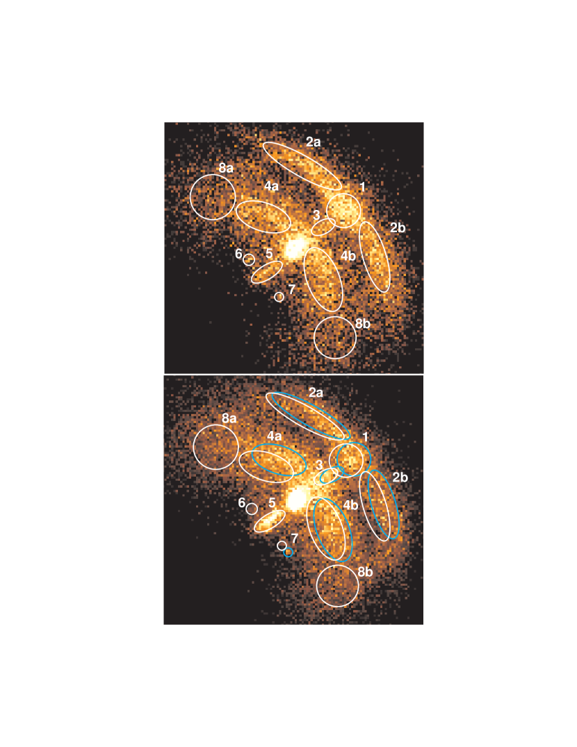
Figure 1: ACIS-S images of a central part ($57^{\prime\prime}\times 55^{\prime\prime}$) of the Vela PWN of 2000 Apr 30 (top) and Nov 30 (bottom). The pixel size is $0\farcs 492$. The white contours in the top panel define the PWN elements in the first image. In the bottom panel, the white contours correspond to the contours in the top panel, while the blue contours demonstrate the displaced nebular elements in the second observation. The brightest spot is the Vela pulsar.

First CXO observations of the Vela pulsar and its PWN (Pavlov et al. 2000; Helfand, Gotthelf, & Halpern 2001; Pavlov et al. 2001; Kargaltsev et al. 2001) have shown a spectacular fine structure which resembles the Crab PWN — arcs, jets, knots, and diffuse cometary tails (see Fig. 1). The symmetry axis of the PWN image (P.A.$=307^{\circ}\pm 2^{\circ}$), which can be interpreted as the pulsar spin axis, is nearly parallel to the direction of the pulsar proper motion (P.A.$=305^{\circ}$, Bailes et al. 1989). This suggests that the “natal kick” of the pulsar was directed along the rotation axis of the neutron star progenitor (e.g., Lai, Chernoff, & Cordes 2001). The spectra of PWN elements are power laws of different slopes, which vary from $\gamma\simeq 1.3$ for the NW jet and inner arc to $\gamma\simeq 1.7$ for the outer diffuse nebula (Kargaltsev et al. 2001). The X-ray luminosity of the whole nebula in the 0.1–10 keV range is $L_{\rm neb}=(6.0\pm 0.5)\times 10^{32}$ erg s^-1 (for $d=250$ pc — Cha, Sembach, & Danks 1999), only $\sim 10^{-4}$ of the pulsar spin-down luminosity $\dot{E}=6.7\times 10^{36}$ erg s^-1 (vs. 0.045 for the Crab PWN).

First indication on the Vela PWN variability was reported by Helfand et al. (2001) who analyzed two images obtained with the CXO High Resolution Camera on 2000 January 20 and February 21. They noticed a $5\%$ brightening of the outer arc and suggested that it may be connected with the large pulsar glitch of 2000 January 16 (Dodson, McCulloch, & Costa 2000). In this Letter we report new results on X-ray variability of the Vela PWN obtained with the CXO Advanced CCD Imaging Spectrometer (ACIS; Garmire et al. 2001).

2 Observations

Two ACIS observations of the Vela pulsar and its PWN were carried out on 2000 April 30 and November 30 with exposure times 10,577 s and 18,851 s, respectively. In both observations the target was imaged on the back-illuminated chip S3. To image the whole PWN on one chip, the pulsar was offset from the ACIS-S aimpoint by $-1\farcm 5$ along the chip row. To reduce pile-up, we used 1/2 subarray, with a frame time of 1.5 s. For the analysis, we used the pipe-line processed Level 2 data (versions 13.2 and 12.1 for the first and second observations, respectively) and the CIAO software, v.2.0. A detailed analysis of the PWN spectra and morphology will be presented elsewhere (Kargaltsev et al. 2001). Herein we concentrate on comparison of the two observations.

To compare the PWN structures, it is particularly important to co-align the images properly. Since no X-ray point sources, other than the piled-up pulsar, are detected in the $8^{\prime}\times 4^{\prime}$ field of view, we have to rely upon the aspect reconstruction which translates the actual event positions on the chip into sky coordinates. For the processing software versions used, the rms aspect offset (error of celestial location) is smaller than $0\farcs 6$, although in some cases the offset can be as large as $2^{\prime\prime}$. To estimate the errors in our case, we found centroids of radial distributions of pulsar counts, which correspond to $\alpha=8^{\rm h}35^{\rm m}20\hbox{$.\!\!^{\rm s}$}628$, $\delta=-45^{\circ}10^{\prime}34\farcs 93$, and $\alpha=8^{\rm h}35^{\rm m}20\hbox{$.\!\!^{\rm s}$}614$, $\delta=-45^{\circ}10^{\prime}35\farcs 26$, for the first and second image, respectively. The difference of these positions, $0\farcs 36$, is comparable with our estimated centroiding error, $\simeq 0\farcs 5$ (about one ACIS pixel).

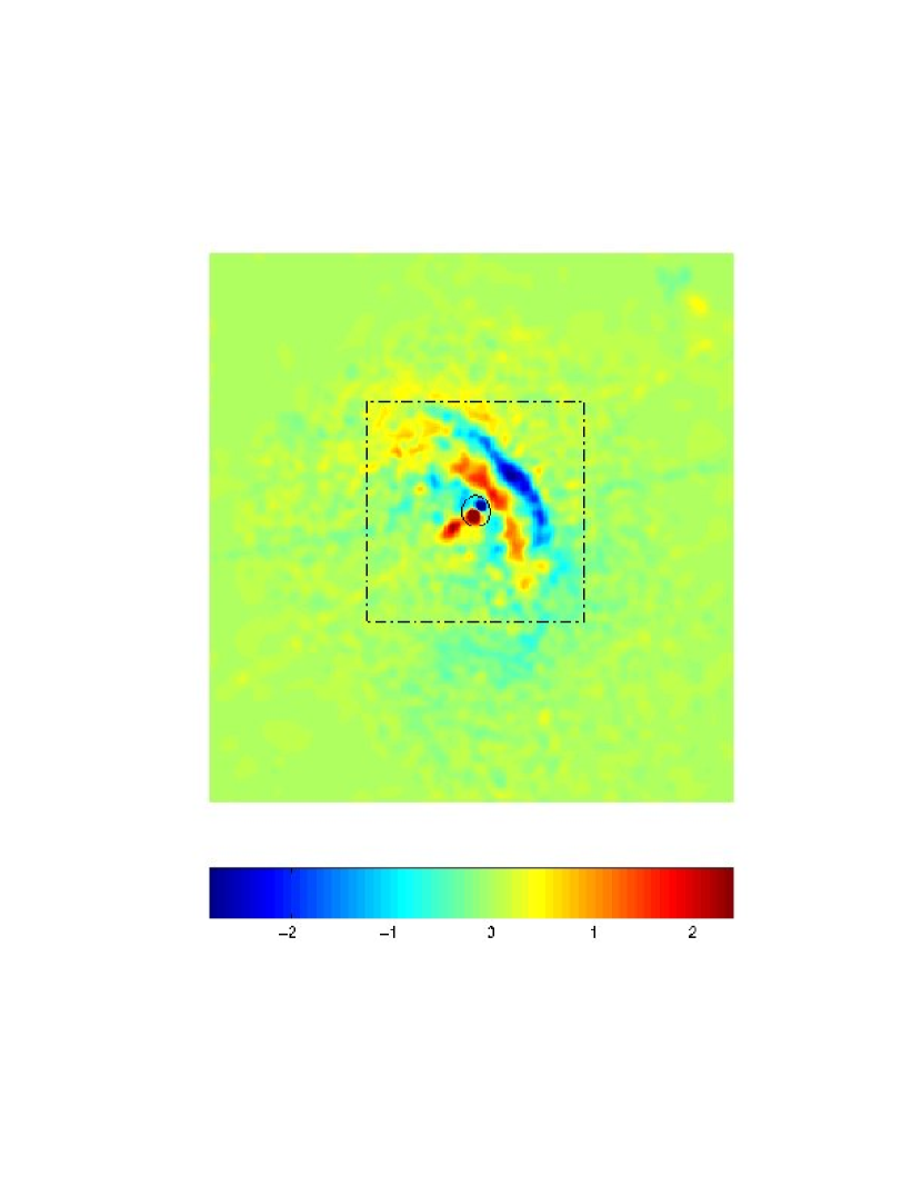
Figure 3: The difference image ($142^{\prime\prime}\times 142^{\prime\prime}$) of the Vela PWN. The color scale is in counts ks^-1 arcsec^-2. The dashed rectangle corresponds to the size of images in Fig. 1. The blue and red structures within the $3\farcs 5$ circle at the center correspond to the “blob” in the pulsar image in the first and second observation, respectively (see text for details). The blue and yellow linear structures are the pulsar trailed images.

The images of the central part of the PWN are shown in the upper and lower panels of Figure 1 for the first and second observation, respectively. The white contours in the upper panel enclose PWN regions chosen for the comparison with the second observation. The regions numbered 1 through 7 enclose well-defined bright features such as the outer arc (2a+2b) with a brightened spot (1) at its apex, NW jet (3), inner arc (4a+4b), SE jet (5), NE knot (6), and SW knot (7). In addition, to examine the variability in the diffuse emission, we define regions 8a and 8b. The white contours in the bottom panel are plotted at the same positions as those in the upper panel. A visual comparison of surface brightnesses within the white contours immediately shows substantial differences between the two images — e.g., the SW jet is brighter, the spot is dimmer, and the NE knot is invisible in the second image. Moreover, we see that some elements appear at different locations — the SW knot moved $2^{\prime\prime}$ westward, and the outer arc shifted by, on average, $2^{\prime\prime}$ north-west from the previous positions. Therefore, we defined new positions of six PWN elements in the second image with blue contours which enclose the same areas as (and are congruent to) the corresponding white contours. To quantify the changes in the surface brightness, we measured the numbers of counts per unit area per unit time within the white and blue contours for the first and second observations, respectively (see Fig. 2), and found that the changes are indeed quite significant for some elements — e.g., $32\%\pm 4\%$ for the SE jet, $-26\%\pm 2\%$ for the spot, and $-19\%\pm 2\%$ for the outer arc (the uncertainties are $1\sigma$ statistical errors), while they are comparable with statistical fluctuations for the others (e.g., for the shifted inner arc). To visualize the spatial distribution of the brightness/morphology change, we scaled the images to the same exposure time (10,577 s), adaptively smoothed them with CIAO task csmooth, and subtracted the first image from the second one. The difference image (Fig. 3) clearly shows the displacements of the arcs and the SW knot, brightening of the SE jet, and dimming the spot and the NE knot. It also shows some brightening (dimming) of the diffuse emission at the NE (SW) outskirts of the PWN and the large displacement, $\approx 8^{\prime\prime}$ toward SW, and shape variation of the filamentary structure in the upper right corner of the image ($75^{\prime\prime}$ NW from the pulsar).

To evaluate systematic errors of the brightness changes, one should take into account that, although the pulsar was imaged at almost the same location on the chip in the two observations, the PWN regions are imaged on different sites because the roll angles were different ($260\hbox{$.\!\!^{\circ}$}3$ and $55\hbox{$.\!\!^{\circ}$}2$). Since the CCD quantum efficiency varies over the chip, this may lead to artificial changes of brightness. To examine this effect, we employed two sets of on-orbit calibration exposures (28 ks and 35 ks, at dates close to those of our observations), during which the ACIS chips were illuminated by on-board radioactive X-ray sources. For each of the calibration datasets, we measured the surface brightnesses of eight domains on the chip where four PWN elements (regions 1, 2b, 4a and 5) were imaged in the first and second observations of the Vela PWN. The differences of the brightnesses of the domains corresponding to the same PWN elements, both in the separate calibration datasets and between the two datasets, are about 2%–3%, comparable to the statistical errors. This puts an upper limit of $3\%$ on both spatial and temporal variability of quantum efficiency within the chip area ($\sim 1^{\prime}\times 1^{\prime}$) where the bright PWN elements were imaged. As an independent test, which additionally accounts for the effect of dither on the exposure times, we constructed exposure maps (e.g., Davis 2001) for the two PWN observations, for an energy of 1 keV close to the maxima of the count rate spectra. Inspection of these maps shows that the effective area varies by about 20% over the whole $8^{\prime}\times 4^{\prime}$ field-of-view, but these large variations are associated with the boundaries between the four chip nodes. Since the PWN elements under investigation are all imaged within the same node 1, the variations are much smaller, $\approx 2\%$. Thus, the large, $\sim 20\%$–30%, brightness changes we detected is not an instrumental effect — they characterize real PWN variations.

We have also measured the mean surface brightnesses in the two observations within a $30^{\prime\prime}$ radius circle (centered on the pulsar). To take into account the above-mentioned nonuniformity, we divided the original images over the exposure maps and found a change of $-3.0\%\pm 0.5\%$. Although this difference looks statistically significant, its magnitude is comparable with possible systematic errors (e.g., caused by inaccuracy of the monoenergetic exposure maps we used).

Comparison of the two observations allows one, in principle, to check whether the pulsar luminosity has changed in 7 months. A change of the luminosity could be caused by the strong glitch of 2000 January 16 because glitch effects can manifest themselves on time scales from weeks to years, depending on the depth where the energy release occurred. We measured the radial count distribution of the piled-up pulsar image and found that its very central part, within a $1^{\prime\prime}$ radius, became brighter by $30\%\pm 5\%$, whereas the brightness did not change at larger radii. In obvious contradiction with this result, the difference in the pulsar countrates, $-8\%\pm 9\%$, estimated from the “trailed images” (one-dimensional images formed during the frame read-outs) is statistically insignificant. Since the trailed images do not suffer from the pile-up, we consider the latter result more reliable. The apparent variation of the central part of the pulsar image is likely caused by a small fluctuation of observing conditions (e.g., focal plane temperature), which may lead to a considerable change in the nonlinear regime associated with strong pile-up. It should also be mentioned that the piled-up images are very asymmetric. In particular, in both observations we see a “blob” of $0\farcs 7$ radius at a distance of $1\farcs 5$ from the center of the pulsar image (see Fig. 3), at an angle of about $22^{\circ}$ from the $Z_{+}$ axis of the spacecraft. The blob is most likely due to a tilt between the telescope mirrors in the innermost shell (Jerius et al. 2001). It can hardly be seen when there is no pile-up because it is much fainter than the core of the point source image, but it appears quite bright in a strongly piled-up image because the pile-up reduces the core brightness.

In addition to the shifts and brightness changes, we have examined the spectral changes of the PWN elements. To characterize the spectra, we use the hardness ratio $h_{1.3}$, defined as the ratio of counts above and below $E=1.3$ keV. For the comparative analysis, this empirical quantity is more convenient than spectral fitting parameters because it does not depend on the spectral model, and does not suffer from uncertainties of the detector spectral response. We see some evidence of hardness changes, up to $+29\%\pm 8\%$ in the SE jet (see Fig. 2), but their statistical significance, $<3.6\sigma$, is not as high as that of the brightness changes.

3 Discussion.

The comparison of the two ACIS observations taken 7 months apart shows that the Vela PWN is by no means static — we have detected considerable brightness changes and/or shifts of some PWN elements, which are likely accompanied by spectral changes. With only two observations carried out, we cannot trace these variations to establish their time scales and velocities. In particular, it is hard to conclude whether the apparent shifts of the arcs and the SW knot are associated with steady motion of matter during the 7 months or are manifestations of wave phenomena, or some instabilities, in the post-shock relativistic plasma. The fact that the NE knot has disappeared and the other PWN elements have changed their brightness implies that the changes are more complicated than simple motion of plasma inhomegeneities.

The remarkable similarity of the Vela and Crab PWN morphologies suggests that their variabilities are driven by similar physical processes. The main distinction between the two PWNe is in their sizes and energetics. In particular, the physical size of the Vela PWN, $\sim 0.1$ pc at $d=250$ pc, is an order of magnitude smaller than that of the Crab PWN, in rough correspondence with the scaling, $r_{s}\propto\dot{E}^{1/2}$, for the shock radius in an ambient medium with a given pressure. This correspondence indicates that typical pressures, $p\sim\dot{E}/4\pi cr_{s}^{2}\sim 10^{-9}$ erg cm^-3, are of the same order of magnitude, which is in agreement with the close values of their equipartition magnetic fields, $B\sim 10^{-4}$ G (Kargaltsev et al. 2001). The similarity of physical parameters of the relativistic plasmas in the two PWNe suggests that typical velocities of MHD waves, presumably responsible for some of the observed variabilities, are also similar. In a relativistic magnetized plasma these velocities depend on the mean energy density $\varepsilon$, magnetization parameter $\sigma=B^{2}/(4\pi\varepsilon)$, and the angle $\theta$ between the wavevector and the magnetic field (e.g., Gedalin 1993). For the conditions expected in the Crab and Vela PWNe, they vary from very low values, $\approx(c/2)\sqrt{3\sigma}|\cos\theta|$, for the Alfven and slow magnetosonic waves at $\sigma\ll 1$, to $\simeq(0.6$–$0.7)c$ for the fast magnetosonic wave at $\sigma\simeq 1$. The fastest speeds observed for the Crab PWN wisps, about $0.5c$ (Hester 1998), are thus close to the upper end of the expected velocity range. If plasma perturbations can propagate with similar velocities in the Vela PWN, the observable shifts $\sim 1^{\prime\prime}$–$2^{\prime\prime}$ can occur in just few days, so that the 7 months between our observations may not be a representative time period to investigate the variations.

The different behavior of the Vela PWN elements suggests that various processes are responsible for the PWN variability — e.g., the apparent motion of the arcs can be caused by wave processes, while the brightness variations of the jets can be associated with large-scale inhomogeneities of the polar outflows. A variety of mechanisms have been invoked to explain the Crab PWN variability — e.g., formation of MHD shock waves in slightly inhomogeneous wind streams (Lou 1998), instabilities driven by synchrotron cooling in the flow (Hester 1995), nonlinear Kelvin-Helmholtz instabilities in the equatorial plane of the shocked wind (Begelman 1999), or cyclotron instabilities of ion rings (Spitkovsky & Arons 2000). To investigate the actual roles of such processes in the Vela PWN, its behavior should be monitored with CXO — other X-ray missions do not have sufficient angular resolution, while observations outside the X-ray band are extremely difficult, if possible at all, because of the PWN faintness in the optical and radio. Moreover, the Vela PWN is more suitable for studying brightness and, particularly, spectral variabilities with the CXO ACIS because it is not as bright as Crab, and its ACIS images do not suffer from pile-up which strongly complicates the data analysis. Thus, future CXO observations of the Vela PWN will provide the unique opportunity to elucidate the physical properties of the relativistic plasmas in PWNe.

Figure 2: Surface brightness vs. hardness ratio $h_{1.3}$ for different PWN regions for the two ACIS-S observations. For the second observation, the values for the regions 1–4 were calculated within the blue contours in the bottom panel of Fig. 1. (The differences would be even larger if exactly the same regions were used for the two observations.)

References

- (1) Bailes, M., Reynolds, J. E., Manchester, R. N., Kesteven, M. J., & Norris, R. P. 1989, ApJ, 343, L53
- Begelman (1999) Begelman, M. C. 1999, ApJ, 512, 755
- (3) Bitenholz, M. F., & Kronberg, P. P. 1992, ApJ, 393, 206
- (4) Bitenholz, M. F., Frail, D. A., & Hankins, T. H. 1991, ApJ, 376, L41
- (5) Cha, A., Sembach, K. M. & Danks, A. C. 1999, ApJ, 515, L25
- (6) Davis, J. E. 2001, ApJ, 548, 1010
- de Jager et al. (1996) de Jager O. C., Harding, A. K., Strickman, M. S. 1996, ApJ, 460, 729
- (8) Dodson, R. G., McCulloch, P. M., & Costa, M. E. 2000, IAU Circ. 7347
- (9) Gaensler, B. M. 2001, in Young Supernova Remnants, eds. S.S. Holt & U. Hwang, AIP, New York (in press; also astro-ph/0012362)
- (10) Garmire, G. P., et al. 2001, ApJS, in preparation
- (11) Gedalin, M. 1993, Phys. Rev. E, 47, 4354
- Greiveldinger & Aschenbach (1999) Greiveldinger, C., & Aschenbach, B. 1999, ApJ, 510, 305
- Harden et al. (1985) Harden, F. R., Grant, P. D., Seward, F. D., & Kahn, S. M. 1985, ApJ, 299, 828
- Helfand et al, (2000) Helfand, D. J., Gotthelf, E. V., & Halpern, J. P. 2001, ApJ, accepted; astro-ph/0007310
- Hester et al. (1995) Hester, J. J., et al. 1995, ApJ, 448, 240
- (16) Hester, J. J. 1998, in Neutron Stars and Pulsars: Thirty Years after Discovery, eds. N. Shibazaki, N. Kawai, S. Shibata and T. Kifune, Univ. Acad. Press (Tokio), p.431
- (17) Jerius, D., et al. 2001, SPIE, in press (http://asc.harvard.edu/cal/Hrma/hrma/psf/index.html)
- Kargaltsev et al, (2000) Kargaltsev, O. Y., Pavlov, G. G., Sanwal, D., Garmire, G. P., & Zavlin, V. E. 2001, ApJ, in preparation
- (19) Lai, D., Chernoff, D. F., & Cordes, J. M. 2001, ApJ, 549, 1111
- Lou (1998) Lou, Y. 1998, MNRAS, 294, 443
- Markwardt & Ögelman, (1998) Markwardt, C. B., & Ögelman, H. 1998, Mem. Soc. Astr. Ital., 69, 927
- (22) Mignani, R., et al. 2001, in preparation
- Ögelman, Finley, & Zimmerman (1993) Ögelman, H., Finley, J. P., & Zimmerman, H.-U. 1993, Nature, 361, 136
- (24) Ögelman H. & Koch-Miramond, L. 1989, ApJ, 342, L83
- (25) Ögelman, H., & Zimmerman, H.-U. 1989, A&A, 214, 179
- (26) Pavlov, G. G., Sanwal, D., Garmire, G. P., Zavlin, V. E., Burwitz, V., & Dodson, R. G. 2000, AAS Meeting 196, #37.04
- (27) Pavlov, G. G., Zavlin, V. E., Sanwal, D., Burwitz, V., & Garmire, G. P. 2001, ApJ Lett, in press (astro-ph/0103171)
- Rees & Gunn (1974) Rees, M. J., Gunn, J. E. 1974, MNRAS, 167, 1
- (29) Scargle, J. D. 1969, ApJ, 156, 401
- Spitovsky & Arons (2000) Spitkovsky, A., & Arons, J. 2000, in Pulsar Astronomy - 2000 and Beyond, eds. M. Kramer, N. Wex, and R. Wielebinski, ASP Conference Series, v.202, p.507
- (31) Weisskopf, M. C., et al. 2000, ApJ, 536, L81
- Willmore et al. (1992) Willmore, A. P., et al. 1992, MNRAS, 254, 139