A Method for Determining the Star Formation History of a Mixed Stellar Population

Abstract

We present a method to determine the star formation history of a mixed stellar population from its photometry. We perform a chi-squared minimization between the observed photometric distribution and a model photometric distribution, based on theoretical isochrones. The initial mass function, distance modulus, interstellar reddening, binary fraction and photometric errors are incorporated into the model, making it directly comparable to the data. The model is a linear combination of individual synthetic color-magnitude diagrams (CMDs), each of which represents the predicted photometric distribution of a stellar population of a given age and metallicity. While the method is similar to existing synthetic CMD algorithms, we describe several key improvements in our implementation. In particular, we focus on the derivation of accurate error estimates on the star formation history to enable comparisons between such histories, either from different objects, or from different regions of a single object. We present extensive tests of the algorithm, using both simulated and actual photometric data. From a preliminary application of the algorithm to a subregion of the Large Magellanic Cloud (LMC), we find that the that the lull in star formation observed among the LMC’s cluster population between 3 and 8 Gyr ago is also present in the field population. The method was designed with flexibility and generality in mind, and we make the code available for use by the astronomical community.

1 Introduction

A quantitative understanding of the physical processes governing star formation is a critical component of galaxy evolution research. A key step toward this understanding is the determination of detailed star formation histories of local galaxies, in which the stellar populations can be resolved. The star formation history (SFH) of a galaxy is defined by its star formation rate as a function of both age and metallicity. Detailed knowledge of a galaxy’s SFH will enable the investigation of several issues in galaxy evolution, including the chemical enrichment of galaxies, galaxy interactions as star formation triggers, the role of stellar dynamics, and the self-propagation of star formation. In addition, the study of local galaxies provides a basic calibration for the study of more distant, unresolved galaxies.

The determination of SFHs from the resolved stellar photometry of local group galaxies is a rapidly evolving area of research. Pioneering work in this area began by inferring a galaxy’s past star formation rate based on the presence of stars in specific evolutionary stages. For example, Cepheid variables (Baade & Swope, 1963; Gaposchkin, 1974) and other supergiants (Kontizas & Kontizas, 1987) have been used to trace relatively recent star formation activity, while carbon stars (Aaronson, 1986; Costa & Frogel, 1996), asymptotic giant branch stars (Frogel & Blanco, 1983; Gallart et al., 1999a), RR Lyrae stars (Baade & Swope, 1961; Saha et al., 1986), and white dwarfs (Noh & Scalo, 1990) have been used as tracers of older star formation. In contrast, classical isochrone fitting to a color-magnitude diagram (CMD), which is based on utilizing a range of stellar types, can be used to highlight the presence of a population of a given age and metallicity (for a recent example, see Mould, 1997). However, this method is most useful for determining the age and metallicity of star clusters, whose star formation histories are simple delta functions. One can attempt to infer the star formation history of a galaxy from a set of such cluster measurements (Girardi et al., 1995; Olszewski et al., 1996), but it is unclear how the cluster formation rate and the overall star formation rate are related.

These methods provide a crude picture of a galaxy’s SFH, but they cannot be used to quantitatively determine the relative numbers of stars formed as a function of age and metallicity in a mixed population. The methods developed to provide such a quantitative measure of the SFH of mixed stellar populations fall broadly under the category of synthetic CMD fitting. A synthetic CMD is the expected photometric distribution of stars, given a particular SFH, photometric errors, and values for the distance modulus, initial mass function (IMF) slope, binary fraction, and interstellar extinction. All synthetic CMD methods involve the construction of a quantitative fitting statistic, with which synthetic CMDs are compared to an observed CMD. A minimization algorithm is then used to determine the SFH of the observed population by constructing a synthetic CMD that most closely resembles the observed CMD. Some synthetic CMD methods use the main sequence (MS) luminosity function (LF) to construct the fitting statistic (Tosi et al., 1991; Stappers et al., 1997; Holtzman et al., 1997; Ardeberg et al., 1997; Aloisi et al., 1999), while others use the LF of particular post-MS phases of stellar evolution. For example, Dohm-Palmer et al. used the LF of blue supergiant Helium-burning stars to reconstruct the recent SFH of Sextans A (Dohm-Palmer et al., 1997) and GR8 (Dohm-Palmer et al., 1998).

The inclusion of the available color information into a synthetic CMD fitting method began with the R-method (Bertelli et al., 1992; Vallenari et al., 1996b, a; Geha et al., 1998), in which the ratios of the numbers of stars in photometrically-defined evolutionary states (e.g., the ratio of the number of MS stars to red giants) is combined with the LF to determine the SFH. The R-method is the direct precursor to the most recent synthetic CMD fitting methods, in which most (if not all) of the two-dimensional information of the CMD is used to quantitatively discriminate between model SFHs. In these methods, the CMD plane is divided into subregions, and the number of stars present in each subregion of both the observed and synthetic CMDs is recorded. These subregion populations are used to construct the fitting statistic, and determine the best-fit SFH. Detailed descriptions of synthetic CMD methods are given in Tolstoy & Saha (1996), Aparicio et al. (1996), Dolphin (1997), and Hernandez et al. (1999). Examples of synthetic CMD methods applied to local group galaxies include NGC 6822 (Gallart et al., 1996a, b), NGC 185 (Martinez-Delgado et al., 1999), the Pegasus dwarf irregular galaxy (Aparicio et al., 1997a; Gallagher et al., 1998), the Carina dwarf irregular galaxy (Hurley-Keller et al., 1998), Leo A (Tolstoy et al., 1998), Leo I (Gallart et al., 1999b), LGS3 (Aparicio et al., 1997b), and the Large Magellanic Cloud (Holtzman et al., 1999; Olsen, 1999).

In this paper we present our own synthetic CMD-based SFH algorithm. Our algorithm is similar to the methods listed above, with what we consider to be a few key improvements: (1) the algorithm efficiently searches large parameter spaces, making artificial constraints on the SFH (e.g. an imposed chemical enrichment law) unnecessary; (2) it takes full advantage of all available photometric information (the algorithm uses multiple CMDs, and all photometered stars can contribute to the fit); (3) it allows for a more realistic treatment of interstellar extinction that includes both differential extinction and age dependence; (4) it performs a detailed calculation of the uncertainties in the best-fit SFH, based on the $\chi^{2}$ topology of the parameter space surrounding the best-fit minimum; and (5) it is designed with generality and flexibility in mind, so that members of the astronomical community can apply it to their own data, using any set of isochrones.

While the generality and flexibility of the method are important, we present the method in a slightly specialized form in this paper, as a primer for our upcoming analysis of the SFH of the Magellanic Clouds (MC). Since our MC data consist of $UBVI$ photometry, we construct synthetic CMD triplets ($\ub$ vs. $B$; $\bv$ vs. $V$; $V-I$ vs. $I$) for model/data comparison. Unless otherwise noted, our examples also use the distance modulus, IMF, interstellar extinction, binary fraction, and photometric errors appropriate for these data.

We provide a brief overview of the method in §2. In §3, we describe the construction of synthetic CMDs from theoretical isochrones. The minimization algorithm is described in §4. We test the method using both artificial photometry and real data in §5. We summarize the results in §7.

2 Method Description

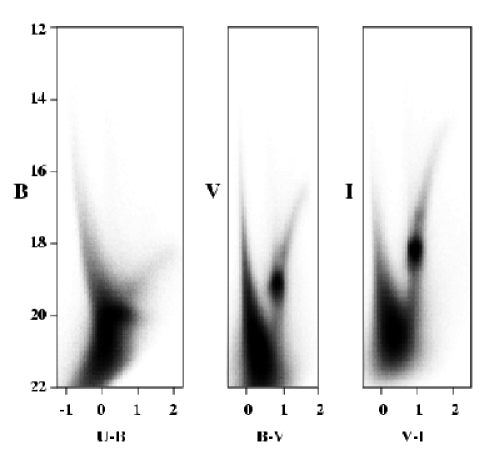
Figure 1: Three projections of the 4-dimensional photometric distribution of 4.1 million stars from our MC Survey. From left to right: the $\ub$ vs. $B$, $\bv$ vs. $V$, and $V-I$ vs. $I$ color-magnitude diagrams. The star formation history of these stars is encoded in their current photometric distribution.

A CMD triplet representing our $UBVI$ photometry of 4.1 million stars from a $4{{}^{\circ}}\times 2.6{{}^{\circ}}$ region of the LMC is shown in Figure 1 (cf. Zaritsky et al. (1997) for a detailed description of the data). Other than the star formation history itself, several external astrophysical parameters influence the observed photometric distribution: the distance of the stellar population, the interstellar extinction, the initial mass function (IMF), the binary fraction, the line-of-sight depth of the population, and the photometric errors. Each of these factors can be independently constrained, leaving only the SFH to be determined.

We begin the SFH reconstruction with a library of theoretical isochrones. Each isochrone describes the intrinsic photometry of a stellar population with a particular age and metallicity. We transform that photometry into a synthetic CMD by accounting for each of the parameters listed above. We consider each synthetic CMD to be an eigen-population: the photometric distribution that would be observed for a stellar population with the age and metallicity of the parent isochrone. While the eigen-populations are not orthogonal, we take steps to ensure that each synthetic CMD represents a unique photometric distribution (cf. §3.4).

A linear combination of these eigen-populations forms a composite model CMD that can represent any SFH. The amplitude associated with each eigen-population is proportional to the number of stars formed at that age and metallicity. The best-fit SFH is described by the set of amplitudes that produces a composite model CMD most similar to the observed photometry. The best-fitting amplitudes are determined using a modified downhill simplex algorithm, described in detail in §4.

A key advantage of this eigen-population approach is that once the library of synthetic CMDs is constructed, we can construct composite model CMDs and compare them to the observed photometry with little computational cost. This efficiency allows us to explore large parameter spaces; we have employed up to 50 independent SFH amplitudes. The efficiency comes at the cost of some flexibility; the external parameters discussed previously (the distance modulus, extinction, IMF, binary fraction, line-of-sight depth, and photometric errors) are incorporated into the synthetic CMDs, and so it is not possible to solve for these parameters and the SFH amplitudes simultaneously. Values for these parameters must be determined (or assumed) prior to the SFH analysis. However, the SFH analysis can be repeated with different parameter values, and the results compared. In this way, we explore the sensitivity of the fit to these external parameters (cf. §5.1.2).

3 Constructing the Synthetic CMDs

3.1 Theoretical Isochrones

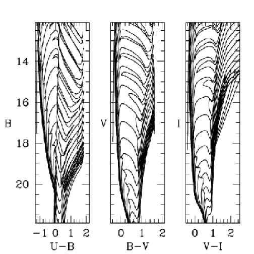
Figure 2: A sample of the Padua Isochrones (Bertelli et al., 1994). Shown are the z=0.008 isochrones, with ages ranging from 4 Myr to 16 Gyr, with logarithmic time steps of 0.2. The isochrones are shown with a distance modulus of 18.5, and with the same photometric limits as Figure 1.

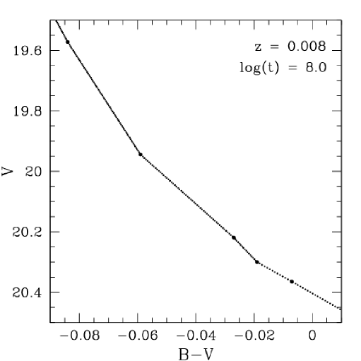
Figure 3: Interpolating the isochrones. Along the main sequence, the Padua isochrones are sparsely populated. The large dots are the original Padua isochrone points; the small dots are our interpolated points.

Reconstructing the SFH of a stellar population from its photometry begins with theoretical isochrones. We use the Padua set of isochrones (Bertelli et al., 1994; Girardi et al., 2000), because it covers a wide range of ages and metallicities, and includes He-burning phases of stellar evolution (i.e., the red clump). A representative sampling of the isochrone photometry is shown in Figure 2. We find that the isochrones are too coarsely sampled along the main sequence for our purposes, so we perform a linear interpolation of the photometry. The interpolated points are evenly distributed along the isochrone with a separation much smaller than the characteristic photometric errors ($\Delta m=0.005$ mag, cf. Figure 3). This default level of interpolation will work well for any currently available data, but like most of the algorithm’s parameters, it can easily be changed if necessary. We then assign to each isochrone point a relative occupation probability (OP) based on an assumed IMF slope:

$$OP_{i}=C\times(M_{i}^{\Gamma}-M_{i-1}^{\Gamma})$$

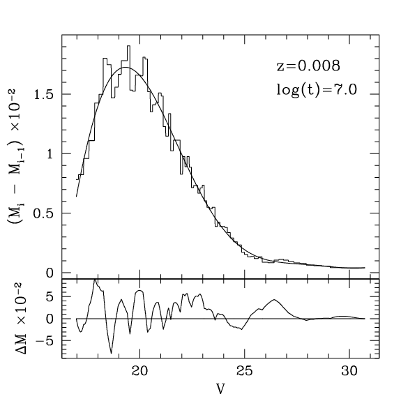
Figure 4: The mass difference between adjacent main sequence isochrone points as a function of $V$ magnitude, for a typical interpolated isochrone (thin line). These mass differences determine the occupation probability of each location along the isochrone. They should be smoothly distributed, because observed luminosity functions of main sequence stars are smooth. The lumpiness is an artifact caused by the fact that the isochrone points follow straight line segments in the CMDs (Figure 3). We correct for this artifact by fitting a smooth curve through the mass differences (heavy line in the figure), and using the mass implied by the curve for each isochrone point.

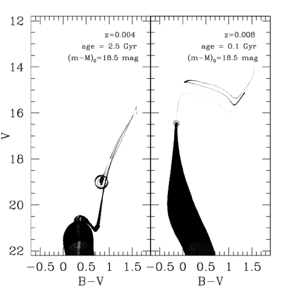
Figure 5: Two sample isochrones plotted with occupation probability represented by point size.

where $M_{i}$ and $M_{i-1}$ are the masses of adjacent isochrone points and $\Gamma$ is the logarithmic IMF slope (unless otherwise noted, we adopt the Salpeter IMF; $\Gamma=-1.35$). $C$ is a normalization constant, with a value chosen such that the total integrated probability over $0.1<M/M_{\odot}<100.0$ is unity. The highly magnified view of the isochrone in Figure 3 reveals that the interpolated points lie along straight line segments in the CMD plane, in approximation of the true isochrone curve. The interpolated masses have similar approximation errors, as illustrated in Figure 4, where we plot the mass differences between adjacent isochrone points as a function of $V$ magnitude. The distribution of approximated mass differences is not smooth, and this lumpiness propagates to the OP values. To remedy this artificial lumpiness, we fit a smooth polynomial through the points of Figure 4, and adopt the mass implied by the curve for each isochrone point. We vary the order of the fitted polynoial from 1 to 12, and determine the best-fit polynomial in each case. Of these candidates, the overall best-fit polynomial is the one with the lowest $\chi^{2}$ value. The fits are examined interactively to ensure that the data are not overconstrained. The resulting mass correction is never more than several hundreths of a solar mass. We smooth only those isochrone points that are fainter than the main sequence turn-off (MSTO). Above the MSTO, the original isochrone points are sufficiently dense that our interpolated points do not deviate significantly from the true isochrone curve. The final distribution of OP values is illustrated in Figure 5, in which the relative OP is represented by point size for two sample isochrones.

3.2 Interstellar Extinction

In previous work, interstellar extinction has typically been modeled as a single mean value, which is simple to implement but implies an unphysical foreground-sheet dust geometry. Harris et al. (1997) investigated the distribution of line-of-sight reddening values toward over 2000 OB stars in a small region of the LMC and found that the distribution of extinction values is much wider than can be accounted for by the photometric errors. Rather, the distribution is consistent with clumpy, exponential line-of-sight distributions for both OB stars and dust, with the scale height of OB stars roughly half that of the dust.

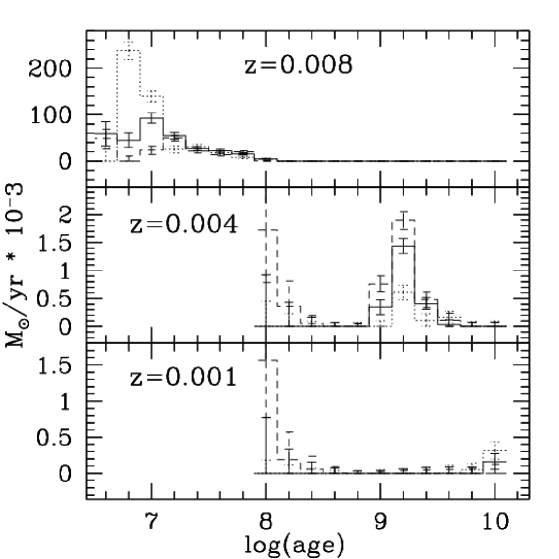
Figure 12: The recovered SFHs of three artificial populations, generated with different values for the IMF slope: $-1.8$ (dashed line), $-1.35$ (solid line) and $-0.9$ (dotted line). In each case, the recovery algorithm used $\Gamma=-1.35$.

Further evidence of differential extinction in the LMC was presented by Zaritsky (1999). Zaritsky demonstrated that extinction in the LMC is population-dependent; hot stars have an average $A_{V}$ extinction that is four times larger than that of cool stars (cf. Zaritsky’s Figure 12). The population dependence of the extinction can be understood as a stellar dynamical effect. The hot stars come from recently formed stellar populations, which tend to be located in regions of the galaxy where the gas and dust density is high. The cool stars are predominantly red giants, and are at least a few billion years old. These stars have dispersed from their dusty formation sites and therefore tend to lie along lines of sight with lower extinction.

For our LMC analysis, the synthetic CMDs incorporate an age-dependent extinction: stars from young isochrones ($\log(t)<7.0$) are assigned extinction values drawn randomly from Zaritsky’s hot star sample, and stars in old isochrones ($\log(t)>9.0$) are assigned extinctions drawn from Zaritsky’s cool star sample. Stars of intermediate age can get their extinction value from either sample, with a probability function that varies linearly with $\log(t)$, increasingly favoring the cool star sample as the isochrone age increases. The age divisions are somewhat arbitrary; $\log(t)=7.0$ is roughly the main sequence lifetime of OB stars, and $\log(t)=9.0$ is an approximation of the diffusion timescale of unbound clusters in the LMC (cf. Harris & Zaritsky, 1999). This reddening prescription was developed for use on our MC Survey photometry; the reddening prescription can easily be adjusted by the user to be appropriate for any input data.

3.3 Photometric Errors

Artificial star tests (ASTs) provide an accurate estimate of the photometric errors, as a function of magnitude and color (cf. Stetson & Harris, 1988). A set of artificial stars with known photometry is inserted into the frame, and the frame is analyzed using the standard data reduction pipeline to recover the photometry of all stars, including the artificial stars.

In performing artificial star tests, the artificial stars must not significantly overlap, or the frame’s crowding conditions will not be correctly sampled. To this end, we follow the procedure outlined by Gallart et al. (1999b). We add artificial stars to the frames in a regular grid, separated by 12 pixels (8.4 arcsec) in each direction. Because the median seeing of the MC Survey photometry is 1.4 arcsec, the artificial stars will overlap only beyond their $3\sigma$ radii. Positions for the artificial stars are generated in right ascension and declination, and for each of the $UBVI$ images, we invert the coordinate solution to determine the corresponding pixel coordinates. This procedure ensures that the artificial stars are added to the image for each filter at the same location with respect to the real stars, regardless of any pointing offsets between exposures.

To obtain a statistically robust determination of the photometric errors, the total number of artificial stars added should be significantly larger than the number of real stars detected in the image. Since a single artificial star test typically contains no more than 5-10% of the image’s total star count, several dozen tests must be run on each image. We randomly offset the grid of artificial stellar positions between runs, so that the artificial stars in each run sample unique crowding environments.

It is also necessary to match the frame’s distribution of stellar magnitudes when constructing the artificial star list, because the photometric errors are dependent on the brightnesses and colors of the stellar sample. We construct the artificial photometry by randomly selecting stars from the theoretical isochrones, according to the Salpeter IMF. In addition, we simulate differential extinction for young stellar populations by assigning extinction values randomly between $A_{V}=0.0$ mag and $A_{V}=1.5$ mag for stars younger than 100 Myr. Stars older than 100 Myr are assigned $A_{V}=0.0$ mag. These steps ensure that the distribution of artificial magnitudes grossly matches that of the data frames, for each of our $UBVI$ filters.

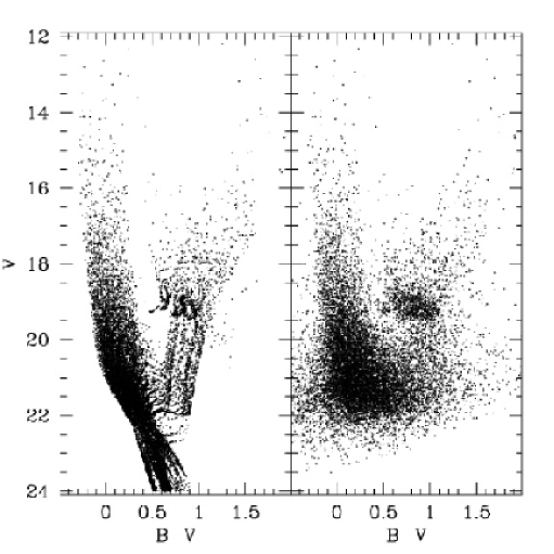
Figure 6: Left: Sample input photometry for an artificial star test. The photometry is drawn from isochrones, assuming a distance modulus of 18.5 mag, a generic SFH, and a Salpeter IMF. In addition, young isochrones are differentially reddened. Note that the main sequences are populated well below the expected faint limit, in order to calculate completeness fractions. Right: The photometry as recovered by our artificial star tests. The tests recover artificial stars from all four of our $UBVI$ frames; only the $\bv$ vs. $V$ CMD is shown here.

Having determined the input coordinates and $UBVI$ magnitudes for the artificial stars, we add them to the images using the DAOPHOT ADDSTAR routine. The resulting images are then processed using the same automated pipeline that we use on the original data. The pipeline applies the coordinate solutions and matches up the $UBVI$ frames to construct a $UBVI$ photometric catalog, containing both artificial and real stars (the combined output list). To extract the recovered artificial star photometry from the combined output list, we use the input catalog of artificial stars and the original stellar catalog containing only real stars. We begin by removing stars from the combined catalog whose coordinates are matched to within 1 arcsec by a star in the original catalog. To avoid accidentally removing artificial stars from the combined list, we further require that the matched stars have similar photometry (within 0.5 mag in each filter) in both lists. Stars in the trimmed output list are then matched with the input artificial stars list, so that we have both the input and recovered $UBVI$ magnitudes for each artificial star. If no match for an artificial star is found in the trimmed output list, that star is flagged as a photometric dropout for calculation of the completeness rate. The input and recovered photometry from a typical artificial stars test is shown in Figure 6.

To determine the dependence of the photometric errors on brightness and color, we divide the artificial star CMDs into magnitude and color bins, and construct the $\Delta m=m_{recovered}-m_{inserted}$ distribution for each bin. One could assign photometric scatter to model stars by identifying the CMD bin in which the model star is found, and drawing randomly from that bin’s $\Delta m$ distribution. However, this procedure results in discontinuities in the photometric scatter at bin boundaries. To ensure that the photometric scatter is smooth throughout the synthetic CMDs, we interpolate between the $\Delta m$ distributions of the four CMD bins surrounding each model star.

3.4 The Synthetic CMDs

Once we have the library of isochrones, the reddening statistics, and the artificial star test results, we construct synthetic CMDs to be compared to the photometric data. Our isochrone library contains 142 isochrones spanning ages from 4 Myr to 18 Gyr, and metallicities between z=0.001 and z=0.008. We decided not to construct an independent synthetic CMD for each of these isochrones, because adjacent isochrones differ in age by only $\Delta\log(t)=0.05$ years, and are often photometrically nearly degenerate. We therefore combine adjacent isochrones into age groups covering $\Delta\log(t)=0.2$ years, reducing the number of independent model parameters to 40. The need to combine isochrones into groups is dictated by the quality of the input data. Data with much smaller photometric errors at faint magnitudes will not require such a constraint (cf. §5.2).

We construct one synthetic CMD triplet ($\ub$ vs. $B$, $\bv$ vs. $V$, and $V-I$ vs. $I$) for each isochrone group. By selecting one million random points from the isochrones’ OP distributions, we construct the predicted photometry for an extremely large stellar population formed at the age and metallicity of the parent isochrones. We construct a large stellar population for each synthetic CMD to ensure that the Poisson noise associated with the model is small compared to the Poisson noise of the data. We apply a distance modulus of 18.5 mag to each of the star’s magnitudes, placing it at the distance of the LMC. In general, the distance modulus applied to the model stars should vary according to a model of the real population’s line-of-sight distribution. However, the line-of-sight depths of the LMC and of the globular clusters we examine in this paper are insignificant, so we apply a single distance modulus in the present work. The model stars are reddened by drawing a random extinction value from the appropriate stellar sample in Zaritsky (1999) (cf. §3.2). We then apply the photometric error model derived from a typical LMC artificial stars test (cf. §3.3). For each model star, we interpolate the completeness fraction from the surrounding CMD bins, and probabilistically remove the star from the population according to this completeness fraction. If the star is not removed, its photometry is scattered by randomly drawing from the interpolated $\Delta m$ distributions in each CMD dimension.

We bin each synthetic CMD into 0.05 mag $\times$ 0.05 mag pixels. The pixel values are computed as: $p(i)=N(i)*f/N$, where $p(i)$ is the value of pixel $i$, $N(i)$ is the number of model stars observed in pixel $i$, $N$ is the total number of stars in the model population, and $f$ is the fraction of stars represented in the current isochrone:

$$f=\frac{M_{max}^{\Gamma}-M_{min}^{\Gamma}}{100.0^{\Gamma}-0.1^{\Gamma}}$$

Each isochrone covers a finite range in masses that is a subset of the full mass interval over which stars form. Stars outside the mass range covered by the isochrone have either evolved to non-luminous end states, or are less massive than the smallest mass represented in the Padua isochrones, $M_{min}=0.6M_{\sun}$. After this normalization, the pixel values represent the fraction of all stars formed in the synthetic population that currently occupy each CMD pixel. This normalization is critical, as it provides a direct transformation from the number of stars observed in a CMD to the number of stars formed in a population.

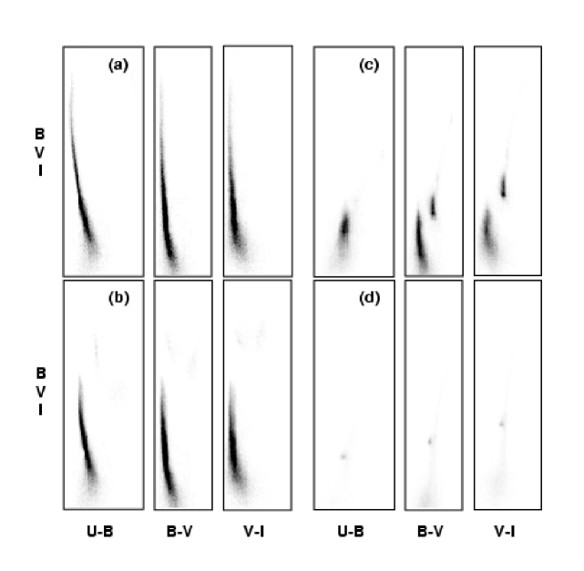
Figure 7: A sampling of our synthetic CMD library. The limits on each CMD are as in Figure 1. Four CMD triplets are shown: (a) z=0.008, age=$10^{7}$ yr; (b) z=0.008, age=$10^{8}$ yr; (c) z=0.004, age=$10^{9}$ yr; (d) z=0.001, age=$10^{10}$ yr;

This procedure results in a library of synthetic CMD triplets, one triplet for each isochrone group. A representative sample of the synthetic CMDs is shown in Figure 7. Pixel values in the older synthetic CMDs are smaller, illustrating the normalization outlined above. A composite model CMD is constructed as a linear sum of the synthetic CMDs. Each term in the sum is assigned an amplitude coefficient that represents the number of stars formed at the age and metallicity of that synthetic CMD. We impose a positivity constraint on these amplitudes to avoid unphysical negative star formation rates. By varying the amplitudes, we are able to construct a model CMD that represents the observed photometry of a stellar population with any arbitrary SFH.

4 The Minimization Algorithm

The amplitude coefficients modulating the synthetic CMDs form a N-dimensional parameter space of possible SFHs. Given an observed CMD triplet, we assign a fitting statistic ($\chi^{2}$) to each set of amplitudes that describes how well that model’s CMDs match the observed CMDs. The best-fitting SFH is then described by the set of amplitudes with the lowest $\chi^{2}$ value. We construct $\chi^{2}$ as the sum:

$$\chi^{2}=\sum_{i}\frac{(N_{D_{i}}-N_{M_{i}})^{2}}{N_{D_{i}}}$$

where $N_{D_{i}}$ is the number of stars observed within the $i$th subregion of the CMD triplet, and $N_{M_{i}}$ is the number of stars in the composite model, in the same subregion. The division of the CMDs into subregions is specified by the user. We have experimented both with a uniform gridding of the CMD planes into boxes covering $0.25\times 0.25$ mag, and with an adaptive grid that is fine in photometrically dense regions like the red clump and main sequence, and coarse in photometrically sparse regions. We found the best-fit SFH to be relatively insensitive to our choice of gridding strategy; because it is simpler, we use the uniform gridding in the present work. The grid size of 0.25 mag was chosen as detailed enough that we can discriminate among similar SFH models, but coarse enough that we will not need to interpolate between isochrones. Subregions in which $N_{D_{i}}=N_{M_{i}}=0$ do not contibute to the sum. If $N_{D_{i}}=0$, but $N_{M_{i}}>0$, we replace $N_{D_{i}}$ with $1.0$ in the denominator, as an approximation of the Poisson error when $N=0$.

Previous SFH studies have had sufficiently few parameters that a brute force minimization algorithm, in which all of parameter space is tested, was practical. However, we are constructing parameter spaces with up to 51 dimensions (51 independent isochrone amplitudes), so searching all of parameter space is not possible. Instead, we employ a downhill simplex $\chi^{2}$ minimization algorithm (Press et al., 1992). We start at a random point in parameter space, and construct a simplex about that point. The simplex is a collection of $N_{dim}+1$ parameter locations and their corresponding $\chi^{2}$ values, where $N_{dim}$ is the number of parameter space dimensions. The first point is the original random location, and the remaining points are generated by perturbing the original point by a small fixed amount along each dimension in the parameter space. Thus, a three-dimensional simplex would be a tetrahedron. From the collection of $\chi^{2}$ values, the local $\chi^{2}$ gradient is calculated, and a step in the direction of the gradient is taken. The new local $\chi^{2}$ gradient is calculated, and the process repeats until a minimum is found.

We use two safeguards against settling on local, rather than global, minima. First, when the simplex signals that it has found a minimum, it is expanded in all dimensions, and allowed to reconverge. Once this reconvergence returns the simplex to the original parameter location, our second safeguard is activated. A small step is taken in a random parameter space direction. If the $\chi^{2}$ value of the new location is lower than the minimum candidate, then the candidate was a local minimum. We continue stepping in this direction until an “uphill” step is taken. This is repeated for tens of thousands of random parameter space directions, and the simplex is restarted at the tested location with the lowest $\chi^{2}$ value.

We find that this second safeguard is critical to finding the true global minimum. On its own, the simplex often converges on local minima because it only searches the local parameter space along directions parallel to the $N_{dim}$ parameter axes. As the simplex approaches the minimum, it becomes more important to explore parameter changes where a deviation in one parameter is offset by a complementary deviation in one or more other parameters. In other words, downhill gradients tend to lie along “off-axis” parameter directions near the minimum, but these directions are ignored by the simplex. Therefore, we iterate between converging toward a minimum with the simplex, and searching in random parameter directions for lower $\chi^{2}$ values. The iteration stops only when the search of random directions produces no lower $\chi^{2}$ values. The number of random directions searched is arbitrary, but our choice of $\sim 30000$ directions appears to cover the parameter space sufficiently. Tests in which we increase the number of search directions by a factor of 10 produce the same global minima.

An important issue in such $\chi^{2}$ minimization procedures is whether the best-fit model is a good absolute fit. The canonical determinant is the $\chi^{2}$ value itself: the best-fit reduced $\chi_{\nu}^{2}$ should be roughly unity for a good fit. However, this criterion is rigorously true only if the errors on the fit are Gaussian distributed, which is unlikely in this application. Nevertheless, we can empirically calibrate $\chi_{\nu}^{2}$ by determining the best-fit SFH of model input photometry, constructed from the same isochrones, reddening statistics and crowding effects used to construct the synthetic CMDs. The $\chi_{\nu}^{2}$ values of these artificial data provide an expectation for models that match the data accurately. Despite the non-Gaussian errors, we find that $\chi_{\nu}^{2}\sim 1.0$ is still indicative of a good fit to the data (cf. §5).

Error bars on the SFH amplitudes are determined by identifying the 68% ($1\sigma$) confidence interval on each amplitude. The confidence intervals are determined from the $\chi^{2}$ topology of the parameter space near the minimum. We explore this topology by sampling the $\chi^{2}$ values of selected points near the minimum. These test points are selected in three different ways: First, we vary each amplitude in turn, while holding all others fixed, to determine the uncorrelated error on each amplitude. Next, we vary adjacent pairs of amplitudes while holding others fixed, to determine the pairwise correlated errors. Finally, we vary all amplitudes simultaneously, to determine the general correlated errors. Although the first two strategies are subsets of the more general third strategy, we employ all three strategies to improve the efficiency of the search. Exploring the $\chi^{2}$ topology of a 40-dimensional space is a daunting task; searching along hundreds of thousands of random directions does not necessarily cover the local topology with sufficient density to construct reliable error bars. We employ the uncorrelated errors and pairwise correlated errors to efficiently increase the sampling density in these important cases. In each case, we iteratively step away from the minimum, and determine the $\chi^{2}$ value until $\chi^{2}$ increases to the 68% confidence limit. From the collection of tested points, we select the largest and smallest values for each amplitude as the limits for the errorbars.

5 Testing the Method

We test our SFH minimization algorithm by recovering the SFH of both artificially-generated photometry and real data. The artificial photometry is based on an input SFH, the theoretical isochrones, and reddening and crowding statistics derived from real data. The SFH recovery of these artificial populations allows us to test the performance of our algorithm, and its dependence on parameters such as the reddening distribution, crowding statistics, and the IMF slope. Since we can construct artificial populations with complex SFHs, these tests also illustrate the algorithm’s ability to disentangle mixed stellar populations, and recover the correct SFH. For the real photometry, we use deep globular cluster photometry and selected regions of our Magellanic Clouds survey. The globular cluster data are used to ensure that no systematic bias is introduced by our synthetic-CMD-fitting method, compared to more traditional isochrone-fitting techniques.

5.1 Artificial Photometry Tests

We recover the SFH of artificial stellar populations in the manner described in §4. First, we construct artificial stellar populations using the same values for external parameters (IMF slope, distance modulus, extinction, and binary fraction) as we used to construct the synthetic CMDs. By holding the parameter values fixed, we will highlight any systematic problems with our algorithm, and illustrate the goodness of fit that can be expected from the algorithm, if all the parameters are correctly determined. We then vary the external parameter values in constructing the artificial populations, but we continue to use synthetic CMDs based on the original parameter values. In this way, we examine the effect on the recovered SFH of having incorrectly determined these external parameters.

5.1.1 Parameter-matched populations

Artificial populations constructed using the same external parameter values as adopted in the fitting algorithm allow us to examine the performance of the algorithm directly. In each of these tests, we use canonical values appropriate for the LMC: $(m-M)_{0}=18.5$ mag, $\Gamma=-1.35$, $f_{binary}=0.5$, the population-dependent extinction distribution described in §3.2, and the photometric errors derived from a typical artificial star test from our MC survey data.

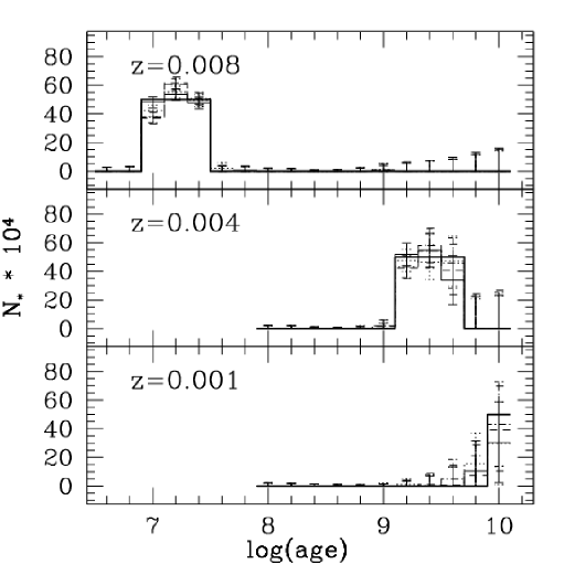
Figure 8: The recovery of a simple, extended-burst SFH. The histograms indicate the number of stars formed in each isochrone group. The isochrones have been divided according to their metallicity. The top panel shows isochrones with z=0.008; the middle panel shows isochrones with z=0.004; and the bottom panel shows isochrones with z=0.001. The input SFH is shown as a heavy solid line. It consists of a young, metal-rich burst, an old metal-poor burst, and an intermediate burst. Four artificial stellar populations are generated from this SFH; the random seed used to select the photometry of the stars is varied in each instance. The best-fit recovered SFH for each of these populations is shown as a dotted line. The errorbars indicate the 68% confidence interval on each amplitude in the $\chi^{2}$ fit.

The first populations are constructed from a simple SFH in which there are three extended bursts of star formation, ranging from old and metal-poor to young and metal-rich. The star formation rate (SFR) is held constant for the duration of each burst. We generate four populations from this SFH, varying both the random seed used to select points along the isochrones, and the random seed that selects the starting set of amplitude values. The recovered SFHs of these populations are shown in Figure 8. We conclude the following from these tests: (1) we have successfully recovered the SFH of the input population, (2) our errorbar estimates are reasonable because they are approximately equivalent to the variance of the amplitudes when different random seeds are used to construct the artificial population, and (3) starting the simplex at different random parameter locations does not affect the determination of the SFH.

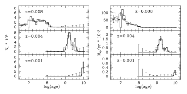
Figure 9: The recovery of a continuous SFH, in which the SFR varies within the age range of individual isochrone groups. The left panels show the SFH as the number of stars formed per isochrone group. The right panels show the SFR, in $M_{\sun}/yr$. The heavy solid line is the input SFH; note the variation of the input SFH within isochrone groups. The dotted line indicates the average input SFR over the age interval of each isochrone group. The thin solid line with errorbars is the best-fit recovered SFH. Note that while the z=0.008 isochrones form a relatively small number of stars, the SFR for these isochrones is relatively high, due to the fact that the time axis is logarithmic.

We simulate more realistic artificial populations by allowing each isochrone to have an independent SFR. The fitting algorithm is inherently unable to fit these populations exactly, because the synthetic CMDs are each composed of multiple neighboring isochrones whose amplitudes are set to be equal to reduce the number of independent isochrones. Figure 9 shows that the algorithm is able to disentangle the mix of many different stellar populations, and it correctly selects the mean SFR over each isochrone group. Note that the simulated SFH shown in Figure 9 has a gap in star formation from 3 to 8 Gyr ago, similar to an age gap suspected in the LMC. This gap is reliably recovered by the algorithm, suggesting that we will be able to answer important questions about the ancient SFH of the Magellanic Clouds.

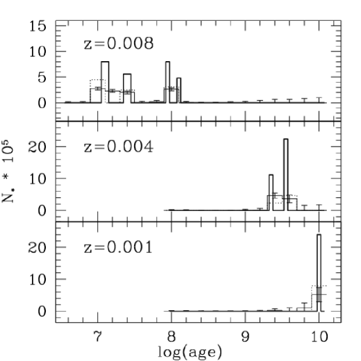
Figure 10: The recovery of a SFH composed of discrete, instantaneous bursts. The heavy solid line shows the input SFH, the dotted line shows the input SFH, averaged over the isochrone groups, and the thin solid line with error bars shows the best-fit recovered SFH.

A more challenging test of the SFH finder is that of an instantaneous burst of star formation, especially one that occurs near the edge of an isochrone group. We construct a stellar population based on several such instantaneous bursts, and recover the best-fit SFH. Figure 10 shows that the recovered SFH again consists of the mean SFR over each isochrone group. The SFH algorithm gives no indication of whether there are variations in the SFR within isochrone groups, even when these are as extreme as an instantaneous burst. If high-frequency variations in the SFR need to be recovered, the isochrone groups need to cover smaller ranges in age (cf. §5.2).

5.1.2 Varying model parameters

The SFH extraction requires knowledge of the following external parameters: the distance modulus, the interstellar extinction, the IMF slope, the photometric errors, and the binary fraction. We next investigate the effects on the extracted SFH of having incorrectly determined these parameters.

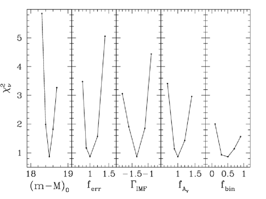
Figure 11: The effect of varying the external parameter’s values on the recovered SFH. For each external parameter, we construct a series of input populations with different parameter values. In recovering the SFH of these populations, however, we assume the standard parameter value appropriate for the LMC. The panels show the resulting reduced $\chi_{\nu}^{2}$ values for each tested parameter. In each case, the best match is found when the correct parameter value is used, but the fit generally degrades slowly as the parameter value changes.

For each external parameter, we construct a series of artificial stellar populations using the same input SFH from Figure 9, varying the parameter’s value for each population. However, the SFH for each population is determined assuming the canonical values for these parameters as described in §5.1.1. The results of these tests are shown in Figure 11. In each case, the lowest $\chi_{\nu}^{2}$ values are found when the parameter value is correctly determined, suggesting that our method can be used to constrain these external parameters. However, the constraint provided by varying these parameters in our models is not generally more precise than is available by other methods.

Some of the parameters remain poorly constrained using either our method or external analyses (notably the IMF slope and binary fraction). The IMF slope in particular is often considered a significant obstacle for synthetic CMD fitting techniques, because it has a large range of plausible values, and the value chosen affects the derived SFH significantly. We examine this sensitivity by plotting the derived SFHs for the same artificial population, assuming three different IMF slopes: $\Gamma=-0.9,-1.35$ and $-1.8$ (cf. Figure 12). Although there are some notable systematic differences, the general form of the derived SFH is remarkably unchanged, considering the wide variance in IMF slope. Differences in IMF slope will have a more significant impact on the SFHs of populations which contain larger numbers of recently formed massive stars. In these cases, we recommend recomputing the SFH with different IMF slope values as we have done. While a strong constraint on the true IMF slope may not be possible, it will at least be clear how sensitive the results are to IMF slope.

5.2 Globular Cluster Photometry

The artificial population tests demonstrate the ability of our algorithm to reliably disentangle the photometry of different stellar populations, and derive an accurate SFH. However, in these tests, it is guaranteed that the synthetic CMDs represent the tested population reasonably well, even in cases where we impose systematic errors (cf. §5.1.2). In applying the method to real populations, this guarantee does not exist. We do our best to accurately account for the distance, interstellar extinction, IMF, and photometric errors, but the only way to rate our accuracy (and that of the theoretical isochrones) is to test the method on real stellar populations whose SFHs have been measured by isochrone-fitting techniques. Globular clusters provide an ideal test case, because they have simple, delta-function SFHs and many have well-established age estimates. We are aware that, like any method that relies on fitting isochrones to observed photometry, there is always a possibility that the models contain unknown systematic errors. Therefore, even if we get the same SFHs for these populations, we have not “proven” their age any more than previous authors have. We are merely attempting to establish that our method gives consistent results with the more traditional isochrone fitting methods. The method was designed so that, as improved theoretical isochrones are published, they can easily be adopted.

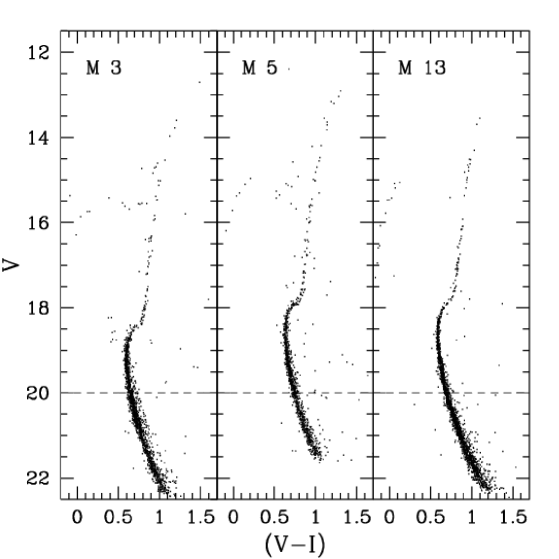
Figure 13: Deep $V-I$ vs. $V$ CMDs for three Galactic globular clusters, from Johnson & Bolte (1998). The dashed line represents our artificial faint limit, imposed to avoid significant completeness effects.

We determine the SFH of three Milky Way globular clusters (M 3, M 5, and M 13) for which deep $V$,$I$ photometry is available (Johnson & Bolte, 1998). CMDs representing this photometry are shown in Figure 13. These data are substantially different than the MC Survey data for which we have designed the method. (1) The photometry is complete well below the ancient main sequence turn off. (2) The photometric errors are small, eliminating the need to combine isochrones into wider age bins. (3) Galactic globular clusters are composed exclusively of old stars. (4) Globular clusters generally do not suffer from differential interstellar extinction. (5) These data are not crowding-limited, so artificial star tests are not absolutely necessary for a reasonable characterization of the photometric errors. (6) The clusters were imaged in only 2 filters ($V$ and $I$), so only one CMD can be constructed.

Our method is easily modified to be appropriate for these data, despite the many differences from our MC Survey data: (1) we modify the time resolution and age range of the synthetic CMD library, covering ages 3 Gyr to 18 Gyr with a resolution of $\Delta\log(t)=0.05$; (2) we employ an extremely simple photometric error model, assuming constant photometric errors of $\sigma_{V}=0.01$ mag and $\sigma_{V-I}=0.02$ mag, based on visual inspection of the CMDs (by using such an ad hoc error model, we continue to stress-test the SFH algorithm by subjecting it to less than ideal conditions); (3) because we have not performed artificial star tests on these data, we avoid the complication of incompleteness by limiting our analysis to stars brighter than $V=20$ mag (dashed line in Figure 13); (4) we adopt simple foreground-only extinction corrections and distance moduli, taken from previous studies of these clusters; (5) we construct the $V-I$, $V$ CMD only; and (6) we divide the CMD using a finer grid, to take advantage of the smaller photometric errors provided by these data. These changes to the method’s functionality were made without having to recompile the code; all operational parameters can be manipulated through input files.

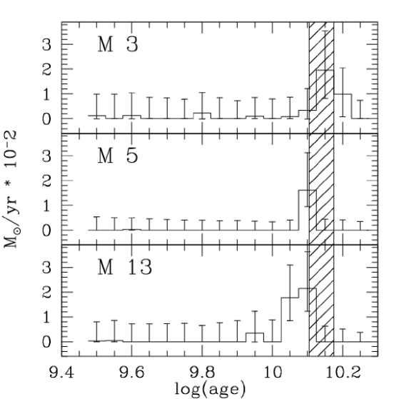
Figure 14: The recovered SFHs of the three Galactic globular clusters. The shaded region indicates the $14\pm 1$ Gyr age for these clusters, as derived by direct isochrone fitting (cf.  Johnson & Bolte, 1998, and references therein). The SFH algorithm was easily modified to be suitable for these data (cf. §5.2). While three metallicities were included in the fit, only the z=0.001 amplitudes are shown. The star formation rate was consistent with zero for the more metal-rich amplitudes.

Once these changes are implemented, the SFH algorithm selects the SFHs shown in Figure 14. These three clusters each have previously published ages of 14 Gyr and metallicities of order z=0.001 (Johnson & Bolte, 1998). Figure 14 shows only the z=0.001 amplitudes. The star formation rates for isochones at z=0.004 and z=0.008 were found to be consistent with zero in each cluster. We conclude that the algorithm has determined the SFH of these clusters quite well ($\Delta t/t=0.1$), considering the crude photometric error model used, and the fact that Johnson & Bolte used a different isochrone set than we used.

5.3 MC Survey Photometry

The algorithm described in this paper was developed to extract the star formation history of the Large and Small Magellanic Clouds from the $UBVI$ photometry of our Magellanic Clouds survey. We are currently reducing and analyzing these data, and the full spatially resolved SFH of the Clouds will be presented in future papers in this series. As a preview of this work, and also to provide an additional test of our algorithm, we present the SFH extraction of selected subsets of our MC survey data.

5.3.1 NGC 1978

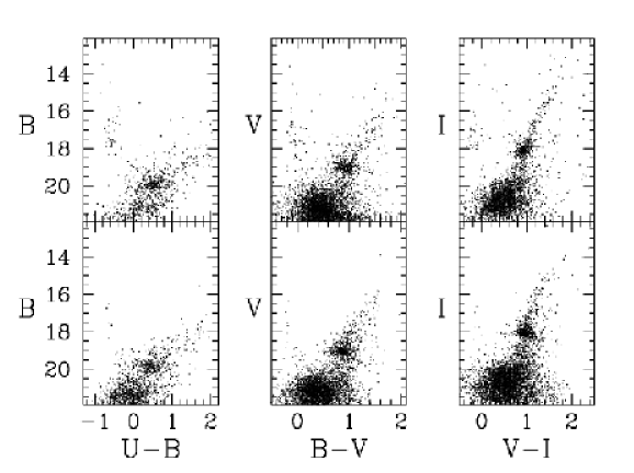
Figure 16: The color-magnitude diagram triplet for NGC 1978, from our MC Survey photometry. Contaminating field stars have been removed from these data through the statistical subtraction of stars in a nearby field of the same size. However, some residual field contamination is visible in the upper main sequence region. Note that the algorithm has attempted to fit this contamination.

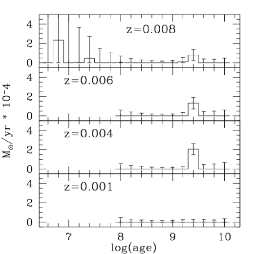
Figure 17: The best-fit recovered SFH for NGC 1978, showing a dominant burst at 2.5 Gyr, with a significant metallicity spread. We compare this result with previous age and metallicity measurements of NGC 1978 in Table 1.

We first present the SFH of the populous star cluster NGC 1978. This is a well-studied star cluster, with numerous age and metallicity determinations in the literature (cf. Table 1). It therefore provides an ideal introduction to our MC Survey photometry because we can check our findings against these previous determinations. We select a rectangular subregion of our Survey, centered on NGC 1978, and spanning 7.2 arcmin in right ascension and declination (cf. Figure 15). The stars within an arcminute of the cluster center are extremely crowded in our data. Because these stars have unacceptably large photometric errors, we exclude them from our sample. We also perform a statistical subtraction of background field stars, using a nearby control field of the same angular size. The statistically cleaned NGC 1978 CMDs are shown in the top panels of Figure 16, and the best-fit SFH for this stellar population is shown in Figure 17. We find a dominant burst with an age of 2.5 Gyr ($\log(t)=9.4$), and a metallicity spanning $-0.7<[Fe/H]<-0.4$. CMDs for the artificial population constructed from this SFH are shown in the bottom panels of Figure 16. The wide range in metallicities found is likely an indication that the method is unable to resolve metallicity differences of $\mathrel{\hbox{\raise 2.15277pt\hbox{$<$}\hbox to0.0pt{\hss\lower 2.15277pt\hbox{$\sim$}}}}0.3$ dex in such data. Synthetic CMDs with z=0.006 are photometrically too similar to both z=0.004 and z=0.008 synthetic CMDs for our method to distinguish between them, given the current data. Therefore, we exclude synthetic CMDs with z=0.006 from our library. Regardless of this issue, the age and metallicity found for NGC 1978 are consistent with the results from previous studies (cf. Table 1), demonstrating that the method has correctly determined the SFH of this population.

5.3.2 LMC field stars

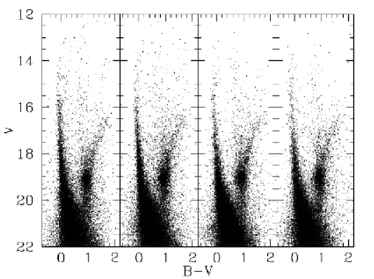
Figure 18: $\bv$ vs. $V$ CMDs of four 20 arcmin $\times$ 20 arcmin subregions of our MC Survey photometry. These fields are adjacent in right ascension. They are north of the LMC bar, centered at approximately ($5^{h}\>27m,-66{{}^{\circ}}\>6^{\prime}$). The differences in the morphologies of these CMDs hint that variations in the SFH are significant on this scale.

As a final demonstration of the algorithm, we determine the SFHs of four contiguous 20 arcmin $\times$ 20 arcmin regions in the northern LMC. The four regions are adjacent in RA, and cover $5^{h}\>21^{m}<\alpha<5^{h}\>33^{m}$ and $-66{{}^{\circ}}\>16^{\prime}<\delta<-65{{}^{\circ}}\>56^{\prime}$. Our MC Survey catalog contains $UBVI$ photometry for about 50000 stars in each of these regions (cf. Figure 18). The full spatially-resolved SFH of both the SMC and LMC, consisting of the individual SFHs of hundreds of regions of this size, will be presented in future papers in this series.

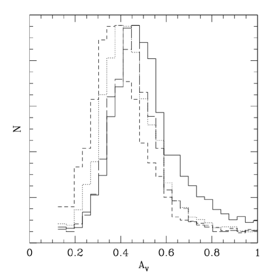
Figure 19: A comparison of the distribution of extinction values toward hot stars in each of the four LMC regions. Each distribution represents our measured extinction values in one of the four adjacent LMC regions, arbitrarily normalized. The extinction varies significantly between these regions, so we construct a unique set of synthetic CMDs for each region, each using its own local extinction distribution.

We construct an independent synthetic CMD library for each region. We use a single artificial star test for all four regions, since each region contains approximately the same density of stars. However, because the reddening varies significantly in these regions (cf. Figure 19), each region uses its own local reddening distribution in constructing the synthetic CMDs. We stress the importance of using an accurate reddening model. Our first attempt at recovering the SFHs of these regions utilized a single reddening distribution. The resulting SFHs had $\chi_{\nu}^{2}$ values that were larger than the current values by a factor of two.

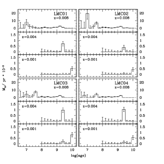
Figure 20: The best-fit recovered SFHs for the four subregions shown in Figure 18.

Once the synthetic CMD libraries are constructed, the algorithm selects the best-fit SFHs shown in Figure 20. For each model, the reduced $\chi_{\nu}^{2}$ is between 7.0 and 9.0; most of the difference is due to a small apparent color offset along the main sequence, in the sense that the models are slightly bluer than the data. The derived SFHs are generally consistent with the recent reconstruction of the LMC SFH by Holtzman et al. (1999); we both find a burst of star formation 2-4 Gyr ago, followed by a lower, continuous star formation rate, up to the present day.

There are several interesting features to note in Figure 20. The recent SFH is highly variable, and changes significantly between regions. There are peaks in the recent star formation rate at 10 and 40 Myr, and the relative strengths of these peaks change systematically from region to region. The SFHs older than $\sim 1$ Gyr are nearly indistinguishable, as expected due to dynamical mixing of stellar populations. The old SFH is dominated by two bursts; a z=0.001 burst at 10 Gyr, and a z=0.004 burst at 2.5 Gyr. This intermediate-age burst has the same age as NGC 1978, which is contained in LMC03. It is possible that these stars are dissolved NGC 1978 members, now populating the LMC field up to 500 pc away from the cluster.

We observe a consistent age-metallicity relation in these regions. The oldest stars have z=0.001, and there is no significant population at this metallicity younger than 2.5 Gyr. This star formation is followed by the single burst with z=0.004, 2.5 Gyr ago. All populations younger than this burst have z=0.008, suggesting a rapid increase in metallicity following the burst. This observed age-metallicity relation is consistent with the analytic model of Pagel & Tautvaisienė (1998).

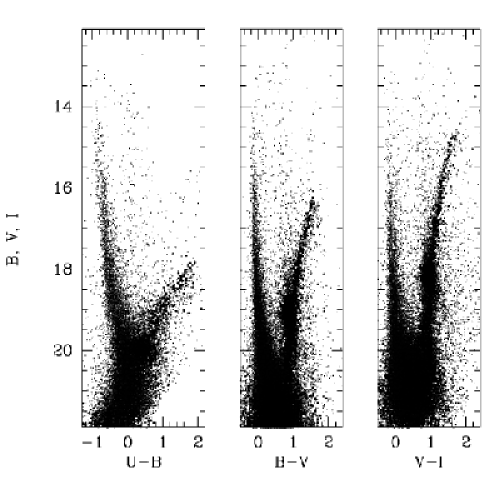
Figure 21: CMD triplet showing the photometry of one of our LMC regions (small points) with a supplemental artificial population (large points) added to fill the age gap between 3 and 8 Gyr.

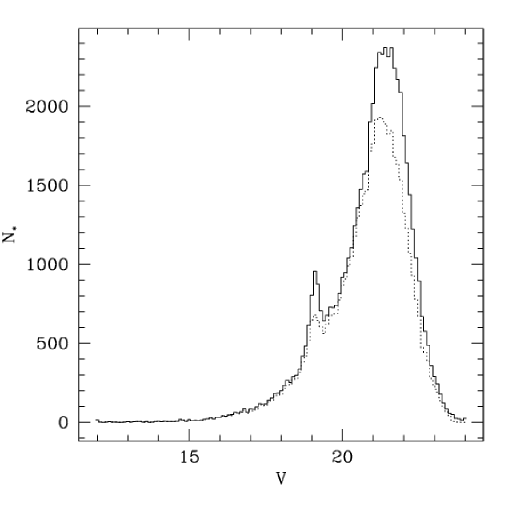
Figure 22: The luminosity function of the LMC region shown in Figure 21, both with (solid line), and without (dotted line) the supplemental population.

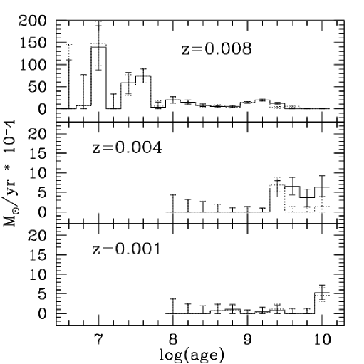
Figure 23: The best-fit recovered SFH of the LMC region shown in Figure 21, both with (solid lines) and without (dotted lines) the supplemental population, added such that the total star formation rate is constant between 2 and 10 Gyr.

Finally, we note that there is no evidence for significant star formation between 3 and 8 Gyr, in agreement with the well-known gap in the ages of LMC clusters. This is a tantilizing result that warrants a closer look. The amplitude error bars suggest a high degree of confidence that the gap exists, yet the gap is not obvious in the CMDs of these populations (Figure 18). What is driving the algorithm to this solution? This question is difficult to address directly, because the algorithm is designed to consider the entire multicolor photometric distribution simultaneously. One could restrict the fit to certain portions of the CMDs, but rather than attempt to second-guess the algorithm, we decided to instead ask the question: how would the CMDs look if the gap did not exist? In Figure 21, we present the observed photometry from one of the LMC regions, with a supplemental, artificial population added to fill the age gap. The size of the population is such that the effective SFR remains approximately constant over the interval from 10 Gyr to 2 Gyr ago. The new population’s metallicity is z=0.004. The supplemental population occupies the red giant branch and faint main sequence regions, but it is not obviously distinct from existing populations in the field. Despite this, the algorithm recovers the correct SFH when given this composite population (cf. Figure 23). The algorithm is able to use small distinctions, such as the position of the red giant branch and the number of main sequence stars as a function of magnitude, to infer the presence of the supplemental population. Because red giant branch morphology is relatively insensitive to age, the main sequence stars likely dominate the determination of ages in the SFH. The supplemental population looks quite subtle in Figure 21. Its presence is more easily seen in Figure 22, which compares the luminosity functions of the original population and the composite population. The significance of faint main-sequence stars in determining the old SFH underscores the importance of accurately estimating photometric errors, completeness rates and the interstellar extinction. Each of these parameters has an important effect on the relative number of faint main sequence stars in the synthetic CMDs.

6 Impact of Systematic Isochrone Errors

The accuracy of theoretical models is a fundamental issue in attempting to reconstruct star formation histories. While we can be confident that some linear combination of theoretical isochrones can accurately reproduce our observed photometry (cf. Figure 16), we still cannot be sure that the correct combination of isochrones produces the best fit. This was our primary motivation in ensuring that any set of isochrones can be used with the method; as improved isochrones are published, they can easily be inserted. Also, because we resolve the CMDs rather coarsely (we use 0.25 mag $\times$ 0.25 mag grid boxes), we do not require absolute precision and accuracy in the isochrones. Other than provide the flexibility to accept new models and robustness against small errors, there is little that can be done to defend against such systematic errors, if they exist. Even if we are reasonably confident that the isochrones are positioned correctly in CMDs (thanks to decades of work comparing isochrone tracks to cluster photometry), a more subtle issue remains: whether the models predict the correct rate at which stars age along evolutionary tracks. If the evolutionary rates are incorrect, the “occupation probabilities” of the isochrones will also be wrong. This possibility is especially troubling for our ancient SFHs: if the RGB region is systematically underpopulated by 25%, then our 10-Gyr amplitude could be just a compensation for the “missing” RGB stars from intermediate-age populations (note, however, that the RGB morphologies of 10-Gyr and 2.5-Gyr populations are not quite the same, which may limit the ability of the ancient population to substitute for the intermediate-age RGB). Such an error could be ruled out by comparing the luminosity function of a single-burst stellar population to that of a synthetic population produced by the best-fit isochrone to the real population. Such a comparison was recently performed by Zoccali & Piotto (2000). They compared the luminosity functions of 18 globular clusters, based on HST photometry, to the predicted luminosity functions from 4 sets of isochrones (including the Padua isochrones that we employ). They conclude that the synthetic luminosity functions match those of the globular clusters, to within HST’s photometric errors.

7 Summary

We have presented a method for determining the star formation history of resolved stellar populations. By adding the effects of distance, interstellar extinction, the initial mass function, photometric errors, and binarity to theoretical isochrones, we construct a library of template synthetic CMDs, each representing the photometric distribution of a stellar population with a single age and metallicity. These synthetic CMDs are then combined linearly and compared quantitatively to observed stellar photometry, to determine the star formation rate as a function of age and metallicity. In this way, present-day stellar populations can be used as a fossil record of a galaxy’s remote history.

Using both artificial photometry and real data, we have extensively tested the robustness and accuracy of the method, under a variety of conditions. We find that the method selects the correct star formation history, even when the external parameters (distance modulus, IMF slope, binary fraction, interstellar extinction, and photometric errors) are imperfectly determined. We also apply the method to four fields in the Large Magellanic Cloud. We find significant spatial variation in the recent star formation history, and a consistent age-metallicity relation in all four fields. We also observe a quiescent era between 3 and 8 Gyr ago, similar to the well-known age gap seen among LMC star clusters.

We will apply the method to the photometry from our survey of the Magellanic Clouds. We have obtained $UBVI$ photometry of tens of millions of stars in each Cloud; for the first time, we have a complete census of the stellar populations down to $V\sim 21$ mag in these two galaxies. By dividing these data into hundreds of subregions, we will construct a map of the star formation history in each of the Clouds. As a demonstration of this work, we present in this paper the star formation histories for four adjacent regions in the northern LMC. These four regions already show significant variation in their star formation histories, and confirm the presence of an extended quiescent era in the LMC’s remote past. The full maps of the SFHs of the Magellanic Clouds will allow us to address many of the outstanding problems in galaxy evolution and the physical processes governing star formation.

The method is useful beyond our immediate plans to map out the SFH of the Magellanic Clouds. The Hubble Space Telescope and large ground-based telescopes have the ability to resolve more distant local group galaxies into individual stars. Galaxies in the local group span a wide range in properties, and recent work has suggested that these galaxies have experienced quite different star formation histories. Our method provides a way to uniformly and quantitatively determine the star formation histories of these systems, so that their histories can be reliably compared, and explanations of the differences can be sought. The algorithm was designed to be easily adaptable to nearly any kind of stellar photometry data, and the code is available for the astronomical community at http://ngala.as.arizona.edu/mcsurvey/SFH

Acknowledgements: D. Z. acknowledges financial support from an NSF grant (AST 96-19576), a NASA LTSA grant (NAG 5-3501), a David and Lucile Packard Foundation Fellowship, and an Alfred P. Sloan Fellowship. J. H. is grateful for fruitful discussions on synthetic CMD fitting methods with Carme Gallart and Jon Holtzman. We thank Jennifer Johnson and Michael Bolte for making their photometry of M 3, M 5, and M 13 available to us.

Table 1: Measurements of NGC 1978

Author	[Fe/H]	age (Gyr)
Present work	$-0.4$–$-0.7$	$2.5\pm 0.5$
Bica et al. (1986)	$-1.1$	6.6
Bomans et al. (1995)	$-0.4$	2.1
Chiosi et al. (1986)	$-0.5$	1.8
de Freitas Pacheco et al. (1998)	$-0.6$	$3.0\pm 1.0$
Elson & Fall (1988)	$\cdots$	2.5
Olszewski et al. (1991)	$-0.41$	$\cdots$
Olszewski (1984)	$-0.5$	2.0

Figure 15: A $V$-band image of a 7.2 arcmin $\times$ 7.2 arcmin subsection of our MC Survey, centered on the populous LMC cluster NGC 1978. These stars provide an ideal test for our SFH algorithm, because several determinations of the age and metallicity of NGC 1978 exist in the literature.

References

- Aaronson (1986) Aaronson, M.: 1986, in Star Forming Dwarf Galaxies and Related Objects, p. 125
- Aloisi et al. (1999) Aloisi, A., Tosi, M., & Greggio, L.: 1999, AJ 118, 302
- Aparicio et al. (1997a) Aparicio, A., Gallart, C., & Bertelli, G.: 1997a, AJ 114, 669
- Aparicio et al. (1997b) Aparicio, A., Gallart, C., & Bertelli, G.: 1997b, AJ 114, 680
- Aparicio et al. (1996) Aparicio, A., Gallart, C., Chiosi, C., & Bertelli, G.: 1996, ApJ 469, L97
- Ardeberg et al. (1997) Ardeberg, A., Gustafsson, B., Linde, P., & Nissen, P. E.: 1997, A&A 322, L13
- Baade & Swope (1961) Baade, W. & Swope, H. H.: 1961, AJ 66, 300
- Baade & Swope (1963) Baade, W. & Swope, H. H.: 1963, AJ 68, 435+
- Bertelli et al. (1994) Bertelli, G., Bressan, A., Chiosi, C., Fagotto, F., & Nasi, E.: 1994, A&AS 106, 275
- Bertelli et al. (1992) Bertelli, G., Mateo, M., Chiosi, C., & Bressan, A.: 1992, ApJ 388, 400
- Bica et al. (1986) Bica, E., Dottori, H., & Pastoriza, M.: 1986, A&A 156, 261
- Bomans et al. (1995) Bomans, D. J., Vallenari, A., & de Boer, K. S.: 1995, A&A 298, 427
- Chiosi et al. (1986) Chiosi, C., Nasi, E., Bertelli, G., & Bressan, A.: 1986, A&A 165, 84
- Costa & Frogel (1996) Costa, E. & Frogel, J. A.: 1996, AJ 112, 2607