Microlensing Constraints on the Frequency of Jupiter-Mass Companions: Analysis of Five Years of PLANET Photometry

Abstract

We analyze five years of PLANET photometry of microlensing events toward the Galactic bulge to search for the short-duration deviations from single lens light curves that are indicative of the presence of planetary companions to the primary microlenses. Using strict event selection criteria, we construct a well defined sample of 43 intensively monitored events. We search for planetary perturbations in these events over a densely sampled region of parameter space spanning two decades in mass ratio and projected separation, but find no viable planetary candidates. By combining the detection efficiencies of the events, we find that, at 95% confidence, less than $25\%$ of our primary lenses have companions with mass ratio $q=10^{-2}$ and separations in the lensing zone, $[0.6-1.6]\theta_{\rm E}$, where $\theta_{\rm E}$ is the Einstein ring radius. Using a model of the mass, velocity and spatial distribution of bulge lenses, we infer that the majority of our lenses are likely M dwarfs in the Galactic bulge. We conclude that $<33\%$ of M-dwarfs in the Galactic bulge have companions with mass $m_{p}=M_{\rm Jup}$ between 1.5 and 4$~{}{\rm AU}$, and $<45\%$ have companions with $m_{p}=3M_{\rm Jup}$ between 1 and 7$~{}{\rm AU}$, the first significant limits on planetary companions to M-dwarfs. We consider the effects of the finite size of the source stars and changing our detection criterion, but find that these do not alter our conclusions substantially.

1 Introduction

The discovery in 1995 of a massive planet orbiting 51 Peg (Mayor & Queloz 1995), followed by the discovery of many more planets orbiting nearby dwarf stars using the same radial velocity technique (Marcy, Cochran & Mayor 2000 and references therein) has focussed both public and scientific attention on the search for extrasolar planets and the experimental and theoretical progress being made in developing other viable detection techniques.

Due to their small mass and size, extrasolar planets are difficult to find. Proposed detection methods can be subdivided into direct and indirect techniques. Direct methods rely on the detection of the reflected light of the parent star, and are exceedingly challenging due to the extremely small flux expected from the planet, which is overwhelmed by stray light from the star itself (Angel & Woolf 1997). Some direct imaging searches have already been performed (Boden et al. 1998), but the future of this method lies in the construction and launching of space-based instrumentation (Woolf & Angel 1998).

Astrometric, radial velocity, and occultation measurements can be used to detect the presence of a planet indirectly. Astrometric detection relies on the measurement of the positional wobble of the stellar centroid caused by the motion of the star around the center of mass of the planet-star system and yields the mass ratio and orbital parameters of the planet-star system. Many attempts to find extrasolar planets in this way have been made, but the measurements are difficult and the detections remain controversial; planned space-based missions astrometric missions such as the Full-Sky Astrometric Mapping Explorer (FAME), the Space Interferometry Mission (SIM), and the Global Astrometric Interferometer for Astrophysics (GAIA) are expected to be substantially more successful. Occultation methods use very accurate photometry of the parent star to detect the small decrease in flux ($\lesssim 1\%$) caused by a planet transiting the face of the star (Borucki & Summers 1984; Hale & Doyle 1994). Many occultation searches are currently being conducted (Deeg et al. 1998; Brown & Charbonneau 2000), with important new limits being placed on planetary companions in 47 Tuc (Gilliland et al. 2000). Recently, one of the extrasolar planets detected via radial velocity surveys was also found to transit its parent star, yielding a measurement of the mass, radius, and density of the companion (Charbonneau et al. 2000; Henry et al. 2000). Spaced-based missions are being planned to increase the sensitivity to low-mass planets (COROT, Deleuil et al. 1997; KEPLER, Borucki et al. 1997). By far the most successful indirect method for discovering planets has been the Doppler technique, which employs precise radial velocity measurements of nearby stars to detect Doppler shifts caused by orbiting planets. Several teams have monitored nearby stars with the aim of detecting the Doppler signal of orbiting planets (McMillan et al. 1993; Mayor & Queloz 1995; Butler et al. 1996; Cochran et al. 1997; Noyes et al. 1997; Vogt et al. 2000). To date these groups combined have discovered over 50 extrasolar planets, with new planetary companions being announced every few months. Several exciting discoveries using the radial velocity technique include the first detection of extrasolar planetary systems (Butler et al. 1999; Marcy et al. 2001a; Marcy et al. 2001b; Fischer et al. 2002) and the detection of planets with masses below that of Saturn (Marcy, Butler, & Vogt 2000).

These detection techniques are complementary to one another both in terms of their sensitivity to planetary mass and orbital separations and the specific physical quantities of the planetary system that they measure. All share two distinct advantages: the experiments are repeatable and, due to their reliance on flux measurements of the parent star or the planet itself, they are sensitive to stars in the solar neighborhood where follow-up studies can be easily pursued. For example, spectroscopic follow-up studies may enable the detection of molecules commonly thought to be indicative of life, such as water, carbon dioxide, and ozone (Woolf & Angel 1998). This advantage is linked to a common drawback: most of the searches can be conducted only on a limited number of nearby stars, and are thus unable to address questions about the nature of planetary systems beyond the immediate solar neighborhood. In addition, most of the methods (astrometry, radial velocity and occultation) can only probe companions with orbital periods smaller than the duration of the experiment. Furthermore, most are fundamentally restricted to massive planets, for example, radial velocity searches probably have an ultimate limit of $\sim 1~{}{\rm m~{}s^{-1}}$ due to random velocity variations intrinsic to the parent stars (Saar, Butler, & Marcy 1998). Of these methods, only space-based interferometric imaging and transit searches are expected to be sensitive to Earth-mass planets.

Microlensing is a relatively new method of detecting extrasolar planets that overcomes many of these difficulties. Galactic microlensing occurs when a massive, compact object (the lens) passes near the observer’s line of sight to a more distant star (the source). If the observer, lens, and source are perfectly aligned, then the lens images the source into a ring, called the Einstein ring, which has angular radius

$$\theta_{\rm E}=\sqrt{{{4G}\over c^{2}}{M\over D_{\rm rel}}}\simeq 320\mu{\rm as}\left({M\over 0.3~{}M_{\odot}}\right)^{1/2},$$ (1)

where $M$ is the mass of the lens, $D_{\rm rel}$ is defined by,

$${1\over D_{\rm rel}}\equiv{1\over D_{\rm L}}-{1\over D_{\rm S}},$$ (2)

and $D_{\rm L}$ and $D_{\rm S}$ are the distances to the lens and source, respectively. The lens-source relative parallax is then $\pi_{\rm rel}={\rm AU}/D_{\rm rel}$. Note that $\theta_{\rm E}$ corresponds to a physical distance at the lens of

$${r_{\rm E}}=\theta_{\rm E}D_{\rm L}\simeq 2~{}{\rm AU}\left({M\over 0.3~{}M_{\odot}}\right)^{1/2}.$$ (3)

If the lens is not perfectly aligned with the line of sight to the source, then the lens splits the source into two images. The separation of these images is $\sim 2\theta_{\rm E}$ and hence unresolvable. However, the source is also magnified by the lens, by an amount that depends on the angular separation between the lens and source in units of $\theta_{\rm E}$. Since the observer, lens, and source are all in relative motion, this magnification is a function of time: a ‘microlensing event.’ The characteristic time scale for such an event is

$${t_{\rm E}}={\theta_{\rm E}\over\mu_{\rm rel}}\simeq 20~{}{\rm days}\left({M\over 0.3~{}M_{\odot}}\right)^{1/2},$$ (4)

where $\mu_{\rm rel}$ is the lens-lens relative proper motion, which we have assumed to be typical of events toward the Galactic bulge, $\mu_{\rm rel}=25~{}{\rm km}\,{\rm s}^{-1}~{}{\rm kpc}^{-1}$.

If the primary lens has a planetary companion, and the position of this companion happens to be near the path of one of the two images created during the primary event, then the planet will perturb the light from this image, creating a deviation from the primary light curve. The duration $t_{\rm p}$ of the deviation is roughly the time it takes the source to cross the Einstein ring of the planet, $\theta_{\rm p}$. From equation (1), $\theta_{\rm p}=(m_{p}/M)^{1/2}\theta_{\rm E}$, where $m_{p}$ is the mass of the planet. Therefore, from equation (4), $t_{\rm p}=(m_{p}/M)^{1/2}{t_{\rm E}}$, or

$$t_{\rm p}=\sqrt{q}{t_{\rm E}}$$ (5)

where $q\equiv m_{p}/M$ is the mass ratio of the system. For a Jupiter/Sun mass ratio ($q\simeq 10^{-3}$), the perturbation time scale is ${\cal O}({\rm day})$. Since the perturbation time scale is considerably less than ${t_{\rm E}}$, the majority of the light curve will be indistinguishable from a single lens. Hence the signature of a planet orbiting the primary lens is a short-duration deviation imposed on an otherwise normal single lens curve.

Because microlensing relies on the mass (and not light) of the system, planets can be searched for around stars with distances of many kiloparsecs. Also, the sensitivity can, in principle, be extended down to Earth-mass planets (Bennett & Rhie 1996). Finally, orbital separations of many AU can be probed immediately, without having to wait for a full orbital period. The primary disadvantages of microlensing searches for planets are that the measurements are not repeatable and there is little hope for follow-up study of discovered planetary systems.

Mao & Paczyński (1991) first suggested that microlensing might be used to find extrasolar planets. Their ideas were expanded upon by Gould & Loeb (1992), who in particular noted that if all stars had Jupiter-mass planets at projected separations of $\sim{r_{\rm E}}$, then $\sim 20\%$ of all microlensing events should exhibit planetary perturbations and that the detection probability will be highest for planets with projected separations lying within $[0.6-1.6]\theta_{\rm E}$ of the primary, the “lensing zone.” Since these two seminal papers, the theoretical basis of planetary microlensing has developed rapidly. Numerous authors have studied detection probabilities and observing strategies incorporating a variety of new effects (Bolatto & Falco 1993; Bennett & Rhie 1996; Peale 1997; Sackett 1997; Griest & Safizadeh 1998; Gaudi, Naber, & Sackett 1998; Di Stefano & Scalzo 1999a, b; Vermaak 2000; Han & Kim 2001; Peale 2001). Notably, Bennett & Rhie (1996) found that the detection probability for Earth-mass planets could be appreciable ($\sim 2\%$), and Griest & Safizadeh (1998) found that for high magnification events the detection probability can be nearly 100% for Jovian planets in the lensing zone. Gaudi & Gould (1997), Gaudi (1998) and Gaudi & Sackett (2000) all discussed extracting information from observed microlensing events. In particular, Gaudi & Sackett (2000) developed a method to calculate the detection efficiency of observed datasets to planetary companions; this method is employed extensively here. Planetary microlensing has been placed in the global context of binary lensing by Dominik (1999b), and studied via perturbative analysis by Bozza (1999, 2000a, 2000b).

On the observational front, progress has been somewhat slower. This is primarily because the survey collaborations that discover microlensing events toward the Galactic bulge, EROS (Derue et al. 1999), MACHO (Alcock et al. 1997a), and OGLE (Udalski et al. 2000), have sampling periods that are of order or smaller than the planetary perturbation time scale, $t_{\rm p}$. However, soon after these searches commenced, these collaborations developed the capability to recognize microlensing events in real time (Alcock et al. 1996; Udalski et al. 1994), thus allowing publically available alerts of ongoing events. In response to this potential, several “follow-up” collaborations were formed: GMAN (Pratt et al. 1996; Alcock et al. 1997b), PLANET (Albrow et al. 1998) and MPS (Rhie et al. 1999a), with the express purpose of intensively monitoring alerted events to search for deviations from the standard point-source point-lens (PSPL) light curve, and in particular the short duration signatures of planets. The feasibility of such a monitoring campaign was demonstrated in the 1995 pilot season of PLANET (Albrow et al. 1998), during which we achieved $\sim 2$ hour sampling and few percent photometry on several concurrent bulge microlensing events.

The MPS collaboration used observations of the high-magnification event MACHO 98-BLG-35 to rule out Jovian companions to the primary microlens for a large range of separations (Rhie et al. 1999b). We performed a similar study of OGLE-1998-BUL-14 (Albrow et al. 2000b), demonstrating that companions with mass $>10~{}M_{\rm Jup}$ were ruled out for separations $1-7~{}{\rm AU}$. Our detection efficiency for this event was $\sim 60\%$ for a companion with the mass and separation of Jupiter, thereby demonstrating that a combined analysis of many events of similar quality would place interesting constraints on Jovian analogs. A similar analysis was performed for events OGLE-1900-BUL-12 and MACHO 99-LMC-2 by the MOA collaboration (Bond et al. 2001).

Bennett et al. (1999) claimed to detect a planet orbiting a binary microlens MACHO 97-BLG-41. As we discuss in §4, we exclude binaries with mass ratios $q>10^{-2}$ from our search because of the difficulty of modeling binaries and therefore of making an unambiguous detection of planetary perturbations amongst the wealth of other perturbations that can occur in these systems. Indeed, Albrow et al. (2000a) found that all available data for this event were explained by a rotating binary without a planet.

Rhie et al. (1999b) claimed “intriguing evidence” for a planet with mass ratio $4\times 10^{-5}\leq q\leq 2\times 10^{-4}$ in event MACHO 98-BLG-35. This perturbation had a reduced $\Delta\chi^{2}\sim 21$, far below our threshold of 60. As can be seen from Figure 7, our data set contains many perturbations with $\Delta\chi^{2}\lesssim 50$. As we show in §6.3, based on studies of constant stars, we find that systematic and statistical noise can easily give rise to deviations in our data with $\Delta\chi^{2}\lesssim 60$.

Bond et al. (2001) reanalyzed all available data for MACHO 98-BLG-35 including the then unpublished PLANET data that are now presented here. They found fits for 1–3 planets all with masses $q<3\times 10^{-5}$, with $\Delta\chi^{2}=60$. This mass range is below our search window, primarily because our sensitivity to it is quite low (see §8). In our view, planetary detections in this mass range should be held to a very rigorous standard, a standard not met by $\Delta\chi^{2}=60$ which would be just at our threshold.

Thus, none of these claimed detections (Bennett et al. 1999; Rhie et al. 1999b; Bond et al. 2001) would have survived our selection criteria even if they had been in our data. Therefore, they pose no conflict with the fact that we detect no planets among 43 microlensing events, and are not in conflict with the upper limits we place on the abundance of planets among bulge stars.

Despite the excellent prospects for detecting planets with microlensing, and after more than five years of intensive monitoring of microlensing events, no unambiguous detections of Jupiter-mass lensing companions have been made. These null results broadly imply that such planetary companions must not be very common. In the remainder of this paper we quantify this conclusion by analyzing five years of PLANET photometry of microlensing events toward the bulge for the presence of planets orbiting the primary microlenses. We use strict event selection criteria to construct a well defined subsample of events. Employing analysis techniques presented in Gaudi & Sackett (2000) and applied in Albrow et al. (2000b), we search for the signals of planets in these events. We find no planetary microlensing signals. Using this null result, and taking into account the detection efficiencies to planetary companions for each event, we derive a statistical upper limit to the fraction of primary microlenses with a companion. Since most of the events in our sample are likely due to normal stars in the Galactic bulge, we therefore place limits on the fraction of stars in the bulge with planets.

We describe our observations, data reduction and post-processing in §2. In §3, we describe and categorize our event sample. We define and apply our event selection criteria in §4; this section also includes a description of how our events are fitted with a PSPL model. We summarize the characteristics of our final sample of events in §5. In §6, we describe our algorithm for searching for planetary perturbations (§6.1) as well as various nuances in its implementation (§§6.2.1-6.2.5). We describe our detections (or lack thereof) in §6.3 and our detection efficiencies in §6.4. Our method of correcting for finite source effects is discussed in §7, and we derive our upper limits in §8. We interpret our results in §9, compare our results with other constraints on extrasolar planets in §10, and conclude in §11. Appendix A lists our excluded anomalous events, and Appendix B discusses parallax contamination.

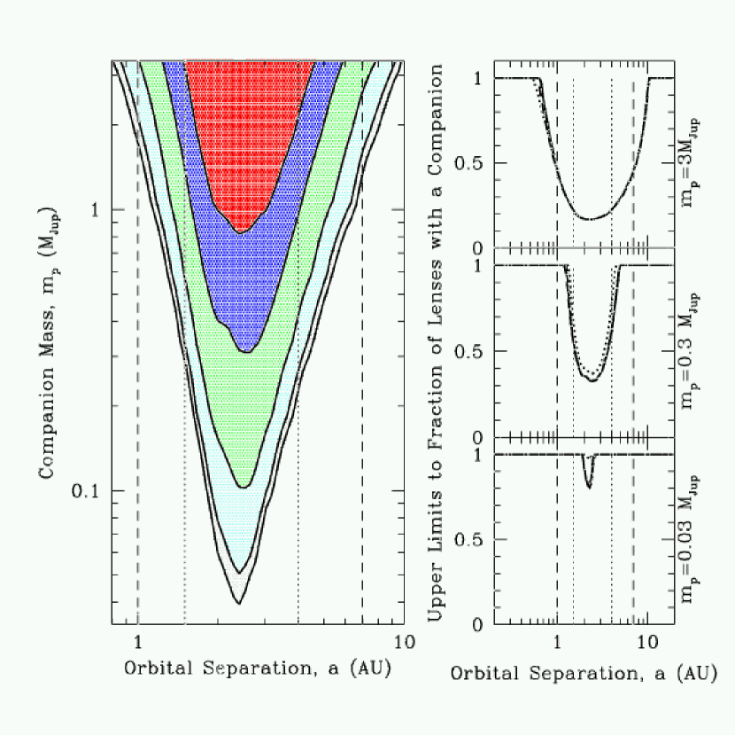
Figure 14: Same as Fig. 12, except we have integrated over all possible orbital inclinations and phases to convert from projected separation to orbital separation, and assumed a primary mass of $M=0.3M_{\odot}$ and a primary Einstein ring radius of ${r_{\rm E}}=2~{}{\rm AU}$.

This paper is quite long, and some of the discussion is technical and not of interest to all readers. Those who want simply to understand the basic reasons why we conclude there are no planets and understand our resulting upper limits on companions should read §3, and §§8-11. Those who want only the upper limits and their implications should read §§10 and 11, especially focusing on Figures 14 and 15. A brief summary of this work is given in Albrow et al. (2001b).

2 Observations, Data Reduction, and Post-Processing

Details of the observations, detectors, telescopes, and primary data reduction will be presented elsewhere (Albrow et al. 2001d). Here we will summarize the essential aspects of the observations and primary data reduction, and discuss only our post-processing in detail.

The photometry of the microlensing events presented and analyzed here was taken over five bulge seasons starting from June of 1995 and ending in December 1999, with a few scattered baseline points taken in early in 2000. These data were taken with six different telescopes: the CTIO 0.9m, Yale-CTIO 1m, and Dutch/ESO 0.91m in Chile, the SAAO 1m in South Africa, the Perth 0.6m near Perth, Australia, and the Canopus 1m in Tasmania. Measurements were taken in the broadband filters $V_{J}$ and $I_{C}$ using a total of 11 different CCD detectors.

The data are reduced as follows. Images are taken and flat-fielded in the usual way; these images are then photometered using the DoPHOT package (Schechter, Mateo, & Saha 1993). A high-quality image is chosen for each field, which is then used to find all the objects on the frame. From this “template” image, geometrical transformations are found for all the other frames. Fixed-position photometry is then performed on all the objects in all the frames. The time-series photometry of all the objects found on the original template image is then archived using specialized software designed specifically for this task. This software enables photometry relative to an arbitrarily chosen set of reference stars. We treat each light curve for each site, detector and filter as independent. The number of independent light curves for each event ranges from one to twelve. For the majority of the events, the $V$-band data are reduced using the source positions identified with the $I$-band template image, since, in general, the signal-to-noise is considerably higher in $I$-band and more objects are detected. This improves the subsequent photometry relative to what can be achieved using a $V$-band template.

Once the photometry of all objects in the microlensing target fields are archived, we perform various post-reduction procedures to optimize the data quality. The light curves of the microlensing source stars are extracted using reference stars chosen in a uniform manner. Four to 10 reference stars are chosen that are close to the microlensing source star (typically within $30^{\prime\prime}$) and exhibit no detectable brightness variations. We require that the ratio of the mean DoPHOT-reported error in the measurements of each reference star to standard deviation all of the measurements of the star is approximately unity, with no significant systematic trend over the entire set of observations. Generally, the mean DoPHOT-reported error in a single measurement of a reference star is 0.01 mag. Reference stars are selected for each independent light curve, although typically the set of reference stars is similar for all observations of a particular event. Only those points on the microlensing event light curve with DoPHOT types 11 or 13, and DoPHOT-reported errors $<0.4$ mags are kept. Further data points are rejected based on unreliable reference star photometry as follows. For each reference star, the error-weighted mean is determined and the point that deviates most ($>3\sigma$) from the mean is removed. The errors of the remaining points are scaled to force the $\chi^{2}$ per degree of freedom (d.o.f.) for the reference star light curve to unity. The error-weighted mean is then recomputed, and the entire process repeated until no $>3\sigma$ outliers remain. The outliers are reintroduced with error scalings determined from their parent light curves. Then, for each data point in the microlensing light curve, the $\chi^{2}$ of all the reference stars are summed. If this $\chi^{2}$ is larger than four times the number of reference stars, the data point is discarded. After this procedure, individual light curves are then examined, and light curves for which the microlensing target was too faint to be detected on the template image were eliminated. In addition, individual light curves with less than 10 points are eliminated. Since at least three parameters are needed to fit each light curve (see §4), light curves with fewer than 10 points contain very little information. Finally, a small number ($\lesssim 10$ over the entire dataset) of individual data points were removed by hand. These data points were clearly highly discrepant with other photometry taken nearly simultaneously, and were typically taken under extreme seeing and/or background conditions, or had obvious cosmic ray strikes near the microlensing target. Since there are only a handful of such points, their removal has a negligible effect on the overall sensitivity. Furthermore, these points cannot plausibly be produced by a real planetary signal, but would lead to spurious detections if not removed.

3 General Considerations

During the 1995-1999 seasons, PLANET relied on alerts from three survey teams, EROS (1998-99), MACHO (1995-99), and OGLE (1995; 98-99). During these five years, several hundred events were alerted by the three collaborations combined. Often, there are too many to follow at one time, and PLANET must decide real-time which alerts to follow and which to ignore. Since the event parameters are typically poorly known at the time of the alert, and survey team data are sometimes unavailable, it is impossible to set forth a set of rigid guidelines for alert selection. The entire process is necessarily organic: decisions are made primarily by one (but not always the same) member of the collaboration, and secondarily by the observers at the telescopes, and are based on considerations such as the predicted maximum magnification and time scale of the event, the brightness and crowding of the source, and the number and quality of other events currently being followed. Our final compilation of events does not therefore represent a well defined sample. Some selection effects are present both in the sample of events alerted by the survey teams and the sample of events we choose to follow. Although these selection effects could in principle bias our conclusions, in practice their effects are probably quite minor, since the reasons that an event was or was not alerted and/or monitored (i.e. crowding conditions and/or brightness of the source, number of concurrent events, maximum magnification) are not related to the presence or absence of a planetary signal in the light curve. The one exception to this is the microlensing time scale, which as we show in §5, is typically twice as long in our sample as in the parent population of microlensing events. One might imagine that, since our sample is biased toward longer time scale events, we are probing higher mass lenses. In fact, as we show in §9, it is likely that we are primarily selecting slower, rather than more massive, lenses. Thus the bias toward more massive primaries is small. This is not necessarily a bias, per se, as long as we take care to specify the population of primary lenses around which we are searching for planets. Thus, provided that any a posteriori cuts we make are also not related to the presence or absence of planetary anomalies in the light curves, our sample should be relatively unbiased.

We would like to define a sample of events in which we can search for and reliably identify planetary companions to the primary lenses. The events in this sample must have sufficient data quality and quantity that the nature of the underlying lensing system can be determined. Also, our method of searching for planetary perturbations is not easily adapted to light curves arising from non-planetary anomalies, such as those arising from parallax or equal mass binaries. Therefore, such events must be discarded. The remaining events represent the well-defined sample, which can then be search for planetary companions. In the next section, we describe our specific selection criteria designed to eliminate these two categories of events and the implementation of these criteria used to define our sample. However, for the most part, our events could be placed cleanly into these categories by eye, without the need of detailed modeling or analysis. Examination of our full sample of light curves reveals that the events generally fall into three heuristic categories:

(1)

Poor-quality events.

(2)

High-quality events which are obviously deviant from the PSPL form for a large fraction of the data span, or are deviant from the PSPL form in a manner that is unlikely to be planetary.

(3)

High-quality events which follow the PSPL form, with no obvious departures from the PSPL form.

(4)

High-quality events which exhibit a short-duration deviation superimposed on an otherwise normal PSPL light curve.

Events in the first category are the most plentiful: they consist of events with either a very small number of points ($\lesssim 20$), poor photometric precision, and/or incomplete light curve coverage. Events in the second category are those with high-quality data, in terms of photometric precision, coverage, and sampling. They typically consist of anomalies recognized real-time, and are comprised of both events that deviate from the PSPL form in a way not associated with binary lensing (i.e. finite source effects, parallax, and binary source events), and events arising from roughly equal-mass (mass ratio ${{}_{>}\atop{}^{{}^{\sim}}}0.1$) binary lenses. Events in the third category are high-quality, apparently normal events that follow the PSPL form without obvious deviations. Events in the last category are planetary candidates.

The first two categories correspond to events that should be removed from the sample; events in the last two categories make up the final event sample, and should be analyzed in detail for planetary companions. Of course, some cases are more subtle, and the interpretation of the event is not so clear. In general, however, other deviations from the PSPL form are easily distinguishable from planetary deviations, with two caveats. First, there is no clear division between “roughly equal mass ratio” and “small mass ratio” binary lenses: if the mass ratio distribution of binary lenses were, e.g, uniform between $q=10^{-5}$ and $q=1$, one would expect grossly deviant light curves, light curves with short-duration deviations, and everything in between. In practice, however, this does not appear to be the case, as we discuss below. Second, there exists a class of binary-source events that can mimic the short-duration deviations caused by planetary companions (Gaudi 1998). Detections of short-duration anomalies must therefore be scrutinized for this possibility.

All of the 126 Galactic bulge microlensing events for which PLANET has acquired data during the 1995-1999 seasons are listed in Table 1. A cursory inspection of these events reveals that $\sim 40\%$ clearly belong in category (1), $\sim 11\%$ clearly belong in category (2), and $\sim 25\%$ clearly belong in category (3). The remaining $\sim 24\%$ are marginal events that could be placed in either category (1) or (3). However, no events clearly belong to the last category, i.e., there are no events that have anomalies that are clearly consistent with a low mass-ratio companion. Since we do not see a continuous distribution in the time scale of deviations with respect to the parent light curve time scale, this implies that either the mass ratio distribution is not uniformly distributed between equal mass and small mass ratios or our detection efficiency to companions drops precipitously for smaller mass ratios. In fact, as we show in §6.4, our efficiencies are substantial for mass ratios ${{}_{>}\atop{}^{{}^{\sim}}}10^{-3}$, implying that massive planetary companions are probably not typical. For the remainder of the paper, we will use strict event selection criteria and sophisticated methods of analysis to justify and quantify this statement.

4 Event Selection

The goal of our selection criteria is to provide a clean sample of events for which we can reliably search for planetary deviations and robustly quantify the detection efficiency of companions. Such criteria are also necessary so that future samples of events (and possibly future detections) can be analyzed in a similar manner, and thus combined with the results presented here. Our selection criteria roughly correspond to the categorization presented in §3. Note that any arbitrary rejection criterion is valid, as long as the criterion is not related the presence or absence of a planetary signal in the light curve.

We first list our adopted rejection criteria, and then describe the criteria, our reasons for adopting them, and the procedure to implement them. The three rejection criteria are:

(1)

Non-planetary anomalies (including parallax, finite source, binary sources, and binaries of mass ratio $>0.01$).

(2)

Events for which no individual light curve has 20 points or more.

(3)

Events for which the fractional uncertainty in the fitted impact impact parameter, $u_{0}$, is $>50\%$.

The original sample of 126 events along with an indication of which events were cut and why is tabulated in Table 1. The first criterion eliminates 19 events, the second 32 events, and the third 32 events, for a final sample of 43 events.

As stated previously, criterion (1) is necessary because we do not have an algorithm that can systematically search for planetary companions in the presence of such anomalies. We are confident that the anomalies in the events that we have rejected by criterion (1) are, in fact, non-planetary in origin, based on our own analyses, analyses in the published literature, and a variety of secondary indicators. Descriptions of each of these events and the reasons why we believe the anomaly to be non-planetary in origin are given in Appendix A.

We fit the observed flux $F_{l}$ of observatory/band $l$ and time $t_{k}$ to the microlensing-event model,

$$F_{l}(t_{k})=F_{{\rm S},l}A(t_{k})+F_{{\rm{B}},l}+\eta_{l}[\theta(t_{k})-\theta_{0,l}]$$ (6)

where $A(t_{k})$ is the magnification at time $t_{k}$; $F_{{\rm S},l}$ and $F_{{\rm B},l}$ are the source and blend fluxes for light curve $l$. The last term is introduced to account for the correlation of the flux with seeing that we observe in almost all of our photometry (see Albrow et al. 2000b). Here $\eta_{l}$ is the slope of the seeing correlation, $\theta(t_{k})$ is the full width at half maximum (FWHM) of the point spread function (PSF) at time $t_{k}$, and $\theta_{0,l}$ is the error-weighted mean FWHM of all observations in light curve $l$. For a single lens, the magnification is given by (Refsdal 1964; Paczyński 1986).

$$A_{0}[u(t)]={{u^{2}(t)+2}\over u(t)\sqrt{u^{2}(t)+4}};\qquad u^{2}(t)=\tau^{2}+u_{0}^{2},$$ (7)

where $\tau$ is the “normalized time,”

$$\tau\equiv{{t-t_{0}}\over{t_{\rm E}}}.$$ (8)

Here $t_{0}$ is the time of maximum magnification, ${t_{\rm E}}$ is the characteristic time scale of the event, and $u_{0}$ is the minimum angular separation (impact parameter) between the lens and source in units of $\theta_{\rm E}$. A single lens fit to a multi-site, multi-band light curve is thus a function of $3+3N_{l}$ parameters: ${t_{\rm E}}$, $u_{0}$, $t_{0}$, and one source flux $F_{{\rm S},l}$, blend flux $F_{{\rm B},l}$, and seeing correlation slope $\eta_{l}$ for each of $N_{l}$ independent light curves. For a binary lens, three additional parameters are required: the mass ratio of the two components, $q$, the binary separation $d$ in units of $\theta_{\rm E}$, and the angle of the source trajectory with respect to the binary axis, $\alpha$. Thus for an event to contain more information than the number of free parameters, at least one observatory must have at least 9+1=10 data points. In order for the fit to be well-constrained, considerably more data points than fit parameters are needed. We therefore impose criterion (2): if no independent light curve has at least 20 data points, the event is rejected. The number 20 is somewhat arbitrary, however the exact choice has little effect on our conclusions: a natural break exists such that the majority of events are well above this criterion, and those few events that are near the cut have little sensitivity to planetary perturbations.

All events that pass criterion (2) are fit to a PSPL model [eqs. (6) and (7)]. At this stage, we also incorporate MACHO and/or OGLE data into the fit, when available. To fit the PSPL model, we combine the downhill-simplex minimization routine AMOEBA (Press et al. 1992) with linear least-squares fitting. Each trial combination of the parameters (${t_{\rm E}},{t_{\rm E}},u_{0}$) immediately yields a prediction for $A_{0}(t)$ [eqs. (7) and (8)]. The flux is then just a linear combination of $F_{{\rm S},l}$, $F_{{\rm B},l}$ and $\eta_{l}$ [eq. (6)]. The best fit parameters $a_{i}=(F_{{\rm S},1},F_{{\rm B},1},\eta_{1},F_{{\rm S},2},F_{{\rm B},2},\eta_{2},...)$ can then be found by forming,

$$b_{ij}\equiv\sum_{k}{{1}\over{\sigma^{2}_{k}}}{{\partial F(t_{k})}\over{\partial a_{i}}}{{\partial F(t_{k})}\over{\partial a_{j}}},\qquad c=b^{-1},\qquad d_{i}=\sum_{k}{{F_{k}}\over{\sigma^{2}_{k}}}{{\partial F(t_{k})}\over{\partial a_{i}}},$$ (9)

where the index $k$ refers to a single observation, the sum is over all observations, and $\sigma_{k}$ is the photometric error in the observed flux $F_{k}$. The parameter combination $a_{i}$ that minimizes $\chi^{2}$ is then,

$$a_{i}=\sum_{j}c_{ij}d_{j}.$$ (10)

Occasionally, the values of $F_{{\rm B},l}$ obtained from this procedure are negative. If $F_{{\rm B},l}$ is negative by more than its uncertainty, we apply a constraint to $c_{ij}$ to force $F_{{\rm B},l}=0$. We then use AMOEBA to find the values of (${t_{\rm E}},{t_{\rm E}},u_{0}$) that minimize $\chi^{2}$. Note that since neither MACHO nor OGLE report seeing values, we do not correct their data for seeing correlations.

We know from experience (Albrow et al. 1998, 2000b) that DoPHOT-reported photometric errors are typically underestimated by a factor of $\sim 1.5$. Naively adopting the DoPHOT-reported errors would thus lead one to underestimate the uncertainty on fitted parameters, and overestimate the significance of any detection. However, simply scaling all errors by a factor to force $\chi^{2}/{\rm d.o.f.}$ to unity is also not appropriate, as we find that our photometry usually contains significantly more large ($>3\sigma$) outliers than would be expected from a Gaussian distribution (Albrow et al. 2000b, 2001a). Furthermore, independent light curves from different sites, detectors, and filters typically have different error scalings. Therefore we adopt the following iterative procedure, similar to that used by Albrow et al. (2000b). We first fit the entire dataset for a given event to a PSPL model in the manner explained above. We find the largest $>3\sigma$ outlier, and reject it. We then renormalize the errors on each individual light curve to force $\chi^{2}/{\rm d.o.f.}$ to be equal to unity for that light curve. Next, we refit the PSPL model, find the largest $>3\sigma$ outlier, etc. This process is repeated until no $>3\sigma$ outliers are found. The outliers are then reintroduced, with error scalings appropriate to their parent light curve. We typically find 3 to 6 outliers $>3\sigma$ in the PLANET data and OGLE data, and a larger number for MACHO data (which contain significantly more data points). The median error scaling for PLANET data is 1.4, with $90\%$ of our data having scalings between 0.8 and 2.8. The errors reported by OGLE are typically quite close to correct (scalings of $\sim 1.1$), while MACHO errors are typically overestimated (scalings of $\sim 0.8$).

Once the best-fit PSPL model is found, we determine the uncertainties on the model parameters by forming $c_{ij}$ as in equation (9), except that now the parameters are $a_{i}=(t_{0},{t_{\rm E}},u_{0},F_{{\rm S},1},F_{{\rm B},1},\eta_{1},F_{{\rm S},2},F_{{\rm B},2},\eta_{2},...)$, i.e., we have included ${t_{\rm E}}$, $t_{0}$, and $u_{0}$. The uncertainty in parameter $a_{i}$ is then simply $\delta a_{i}=(c_{ii})^{1/2}$. Note that we include the outliers to determine the uncertainties. As discussed by Griest & Safizadeh (1998) the sensitivity of a light curve to planetary companions is strongly dependent on the path of the source trajectory in the Einstein ring, such that trajectories that pass closest to the primary lens, i.e. events with small $u_{0}$, will have larger sensitivity than events with larger $u_{0}$. Thus, in order to accurately determine the detection efficiency to a given binary lens, the source path in the Einstein ring, $u(t)$, must be well-constrained; poor knowledge of $u(t)$ translates directly into poor knowledge of the sensitivity of the event to planets (Gaudi & Sackett 2000). The values of $u(t)$ for a given dataset are determined from the mapping between flux and magnification, which depends on the source and blend fluxes, and the mapping between the magnification and time, which depends on $u_{0}$, ${t_{\rm E}}$, and $t_{0}$. In blended PSPL fits, all these parameters are highly correlated. Thus, a large uncertainty in $u_{0}$ implies a large uncertainty in other parameters. Thus the uncertainty in $u_{0}$ in a PSPL fit can be used as an indication of the uncertainty in $u(t)$, and thus the uncertainty in the detection efficiency. Furthermore, for a planetary perturbation, the projected separation $d$ is a function of the observables $(t_{0,{\rm p}}-t_{0})/{t_{\rm E}}$, where $t_{0,{\rm p}}$ is the time of the planetary perturbation, while the mass ratio is $q\sim{{t_{\rm p}}/{t_{\rm E}}}$ (Gould & Loeb 1992; Gaudi & Gould 1997), where ${t_{p}}$ is the duration of the perturbation. Therefore the detection of a planet in an event with poorly constrained ${t_{\rm E}}(u_{0})$ would be highly ambiguous, as the neither the projected separation $d$ nor the mass ratio $q$ would be well-constrained. We therefore impose a cut based on the fractional uncertainty in the fitted value of $u_{0}$.

Figure 1 shows the fractional uncertainty $\delta u_{0}/u_{0}$ in the impact parameter versus $u_{0}$ for all events that passed selection criteria (1) and (2). Examination of the distribution of fractional uncertainty in $u_{0}$ for these events reveals a large clump of events with small fractional uncertainty; many scattered, smoothly distributed events with larger uncertainties, and a natural break in the distribution at $\delta u_{0}/u_{0}\approx 50\%$. We therefore adopt $\delta u_{0}/u_{0}=50\%$ for our final event cut. The exact choice for the cut on $\delta u_{0}/u_{0}$ has little effect on our conclusions; as we discuss in §6.4, events with $\delta u_{0}/u_{0}\gtrsim 30\%$ typically have low detection efficiencies. Four classes of events have poorly-constrained $u_{0}$. These are events: for which the data cover only one (usually the falling) side of the event; for which no baseline information is available; that are highly blended; with an intrinsically low maximum magnification. Thus by imposing a cut on $\delta u_{0}/u_{0}$, we eliminate all low magnification events; the event with largest impact parameter in our final sample has $u_{0}=0.61$. Note that the majority of events that fail the cut on $\delta u_{0}/u_{0}$ fall into the first two classes, which emphasizes the need for coverage of the peak and baseline information. In particular, without MACHO and OGLE data, many more events would not have passed this last cut, and our final sample would have been considerably smaller.

After imposing cuts 1 (non-planetary anomalies), 2 (data quantity), and 3 (uncertainty in the impact parameter), we are left with a sample of 43 events. The light curves for these events are shown in Figure 2. In order to display all independent light curves (which in general have different $F_{\rm S}$, $F_{\rm B}$, and $\eta$), we plot the magnification, which is obtained by solving equation (6) for $A_{0}(t)$. Rather than show the magnification as a function of true time, we show the magnification as a function of normalized time $\tau$ [eq. (8)]. When plotted this way, perturbations arising from a given $q$ would have the same duration on all plots [eq. (5)]. Thus the sensitivity of different light curves to companions can be compared directly. In the next section, we describe the properties of these events, paying particular attention to those properties relevant to the detection of planetary anomalies.

5 Event Characteristics

The parameters $t_{0}$, ${t_{\rm E}}$, and $u_{0}$ and their respective $1\sigma$ uncertainties for the final event sample are tabulated in Table 2, along with the percent uncertainty in $u_{0}$. The sensitivity of an event to planetary companions depends strongly on $u_{0}$ (Gould & Loeb 1992; Griest & Safizadeh 1998; Gaudi & Sackett 2000), and thus the exact distribution of $u_{0}$ influences the overall sensitivity of any set of light curves. The time scale is important in that the population of lenses we are probing is determined from the distribution of ${t_{\rm E}}$. In addition, we use ${t_{\rm E}}$ in §7 to estimate the effect of finite sources on planetary detection efficiencies and therefore the effect on our final conclusions. For the current analysis, the parameter $t_{0}$ is of no interest.

In Figure 3, we plot $u_{0}$ against ${t_{\rm E}}$ for our event sample, revealing no obvious correlation between the two. This lack of correlation between ${t_{\rm E}}$ and $u_{0}$ implies that the lenses that give rise to the events with the most sensitivity to planets (i.e., those with small $u_{0}$) comprise a sample that is unbiased with respect to the entire sample of lenses. Given this, we can then inspect the distributions of $u_{0}$ and ${t_{\rm E}}$ independently.

Both the differential and cumulative distributions of ${t_{\rm E}}$ are shown in Figure 3. The median time scale of our events is $\sim 40~{}{\rm days}$, about a factor of two higher than the median time scale for events found by the MACHO and OGLE teams toward the Galactic bulge (Alcock et al. 1997a; Udalski et al. 2000). This is almost certainly a selection effect caused by the fact that longer time scale events are more likely to be alerted before peak magnification, and thus are more likely to be chosen by us as targets for follow-up photometry. This is compounded by the fact that, for short time scale events, we are less likely to get good coverage of the peak, even if they are alerted pre-peak. Events with poor or no peak coverage will often fail our selection criterion of $<50\%$ fractional uncertainty in $u_{0}$. In principle, this deficiency could be partially alleviated by including MACHO and/or OGLE data. However, in practice, we often stop observing the event altogether if we do not get good peak coverage. As we discuss in §9, the primary effect of this selection is a bias toward slower lenses.

We also show in Figure 3 the differential and cumulative distributions of $u_{0}$. The median $u_{0}$ is $\sim 0.2$, and the fraction of high-magnification ($A_{\rm max}>10$) events is $\sim 30\%$. As it is a purely random quantity, the intrinsic distribution of $u_{0}$ should be uniform. The observed distribution of $u_{0}$, however, is clearly not uniform. This is due to a combination of various selection effects. First, faint events are more likely to be detected (and hence alerted) by the survey teams if they have a larger maximum magnification (Alcock et al. 1997a; Udalski et al. 2000). Since there are more faint stars than bright stars, this results in a bias toward smaller impact parameters with respect to a uniform distribution. Second, since events with smaller impact parameters are also more sensitive to planets, we preferentially monitor high-magnification events. This bias does not affect our conclusions, since the value $u_{0}$ is unrelated to the presence or absence of a planetary companion. However, as emphasized by Gaudi & Sackett (2000), it does imply that in order to determine accurately the overall sensitivity of an ensemble of light curves to planetary companions, the actual distribution of observed $u_{0}$ must be used.

Since one of the primary goals of PLANET is to obtain very dense sampling of microlensing events, it is interesting to examine how well this goal has been achieved. In Figure 4, we show the distribution of sampling intervals, that is, the time between successive exposures of a given event. Three peaks are evident. The first at $\sim 6$ minutes is our typical $I$-band exposure time of 5 minutes plus 1 minute of overhead time; this peak is dominated by events that are followed continuously and also pairs of $I$-$V$ data points. The second peak at $\sim 1.5$ hours represents our fiducial sampling interval. The third peak at 1 day arises primarily from sampling of the wings and baselines of light curves. The median sampling interval is $\sim 1.5$ hours, with 90% of all data taken between 5 minutes and 1 day of one another for a given event. What is of particular relevance to the detection of planets is the sampling interval in units of ${t_{\rm E}}$, which is shown in the lower panel of Figure 4. Assuming that at least 10 data points are needed on a planetary perturbation for detection, the sampling interval needed to detect a companion of mass ratio $q$ is approximately,

$$\Delta t=3\times 10^{-3}{t_{\rm E}}\sqrt{{q\over 10^{-3}}}.$$ (11)

Using this formula and comparing to Figure 4, we find that (80%, 65%, 45%, 25%) of our data have sufficient sampling to detect companions of mass ratio ($10^{-2},10^{-3},10^{-4},10^{-5}$). Thus we expect the majority of our data to have sufficient sampling to detect companions with mass ratios $\gtrsim 10^{-4}$. This is not an accident, since PLANET observations are planned to have sensitivity to Jovian mass planets orbiting main sequence stars (Albrow et al. 1998).

The sensitivity of a given light curve to planetary companions is primarily determined by three factors: photometric errors, temporal sampling, and impact parameter. In Figure 5, we plot the median photometric error, $\sigma_{\rm med}$, versus the median sampling interval, $\Delta t_{\rm med}$ for all events; high-magnification ($A_{\rm max}>10$) events are indicated. These are also tabulated in Table 3. High magnification events that occupy the lower left quadrant of Figure 5 will have the highest sensitivity to planetary companions. Of the 13 high-magnification events, all have sufficiently small median sampling intervals to detect $q=10^{-2}$ companions; we therefore expect our sensitivity to such to companions to be quite high. Two high-magnification events have sufficient sampling rates to detect companions with $q=10^{-5}$; however, for companions as small as this, excellent photometry ($\lesssim 2\%$) along with excellent sampling is required to obtain significant efficiency for detection (Bennett & Rhie 1996). No events satisfy both of these requirements ($\sigma_{\rm med}<2\%$ and $\Delta t_{\rm med}/{t_{\rm E}}<10^{-3.5}$). We therefore restrict our attention to $q\geq 10^{-4}$.

Considering the large number of high-magnification events, and the dense sampling and precise photometry, our sample should be quite sensitive to planetary companions, especially those with $q\gtrsim 10^{-3}$. This fact, combined with the fact that no planetary-like perturbations are clearly evident in the light curves, is an indication that such planetary companions are probably not common. In the following sections, we strengthen and quantify this statement.

6 Search for Detections and Calculation of Detection Efficiencies

Although a cursory inspection of Figure 2 reveals no obvious candidate planetary perturbations, such perturbations could be quite subtle, and thus missed by eye. Furthermore, the significance of the lack of planetary perturbations must be quantified. Specifically, the frequency with which planetary companions of given $d,q$ could be detected in individual light curves, the detection efficiency, must be determined. We simultaneously search for planetary signatures in and determine the detection efficiency of individual events using the method suggested by Gaudi & Sackett (2000) and applied to microlensing event OGLE-1998-BUL-14 by Albrow et al. (2000b). We briefly review the algorithm here, but point the reader to these two papers for a more thorough discussion of the method and its application.

6.1 Algorithm

Of the $6+3N_{l}$ parameters (see §4) in a point source binary microlensing fit, $3+3N_{l}$ have analogs in the PSPL fit: ${t_{\rm E}}$, $u_{0}$, $t_{0}$ and one $F_{{\rm S},l}$, $F_{{\rm B},l}$, and $\eta_{l}$ for each of $N_{l}$ independent light curves. The parameters ${t_{\rm E}}$, $u_{0}$ and $t_{0}$ have different meanings in the binary-lens model than in the PSPL model, and depend on the choice of the origin of the binary-lens and the reference mass. For small mass-ratio binaries, however, if one chooses the origin to be the location of the primary lens, and normalizes to the mass of the primary, then the values of these parameters will be quite similar in a binary-lens and single-lens fit to a light curve. Three parameters are not included in the PSPL fit: the mass ratio $q$, the projected separation $d$, and the angle $\alpha$ of the source relative to the binary-lens axis. While $q$ and $d$ are related to the physical nature of the planet-star system, the angle $\alpha$ is a nuisance parameter which is of no physical interest. It is a random geometric parameter and therefore uniformly distributed. However, the value of $\alpha$ does have a significant effect on the amplitude and duration of the planetary perturbation. Thus, some values of $\alpha$ lead to detectable perturbations to the PSPL model, while others do not. Marginalization over $\alpha$ for a given binary lens specified by ($q,d$) therefore determines the geometric detection efficiency $\epsilon_{i}(d,q)$ for event $i$ and such a binary system. Repeating this process for all $(d,q)$ pairs of interest yields the efficiency for all systems. This is the basis of the method of determining the detection efficiency for individual events suggested by Gaudi & Sackett (2000).

Operationally, the procedure to search systematically for planetary signatures and determine $\epsilon_{i}$ for each event is as follows:

(1)

Fit event $i$ to the PSPL model, obtaining $\chi^{2}_{\rm PSPL}$ (§4).

(2)

Holding $d$ and $q$ fixed, find the binary-lens model that best fits light curve $i$ for source trajectory $\alpha$, leaving the $3+3N_{l}$ parameters (${t_{\rm E}},u_{0},t_{0},[F_{\rm S},F_{\rm B},\eta]N_{l}$) as free parameters. This yields $\chi^{2}(d,q,\alpha)$.

(3)

Repeat step (2) for all source trajectories $0\leq\alpha<2\pi$.

(4)

Evaluate the difference in $\chi^{2}$ between the binary and PSPL fits: $\Delta\chi^{2}(d,q,\alpha)\equiv\chi^{2}(d,q,\alpha)-\chi^{2}_{\rm PSPL}$. Compare this to some threshold value $\Delta\chi^{2}_{\rm thresh}$:

(a)

If $\Delta\chi^{2}(d,q,\alpha)<-\Delta\chi^{2}_{\rm thresh}$, then we tentatively conclude we have a detected a planet with parameters $d,q,$ and $\alpha$.

(b)

If $\Delta\chi^{2}(d,q,\alpha)>\Delta\chi^{2}_{\rm thresh}$ then the geometry $(d,q,\alpha)$ is excluded.

(5)

The detection efficiency $\epsilon_{i}(d,q)$ of event $i$ for the assumed separation and mass ratio is then

$$\epsilon(d,q)\equiv{1\over 2\pi}\int_{0}^{2\pi}{\rm d}\alpha\,\,\Theta[\Delta\chi^{2}(d,q,\alpha)-\Delta\chi^{2}_{\rm thresh}],$$ (12)

where $\Theta[x]$ is a step function.

(6)

Repeat steps (2)-(5) for a grid of $(d,q)$ values. This gives the detection efficiency $\epsilon_{i}(d,q)$ for event $i$ as a function of $d$ and $q$, and also yields all binary-lens parameters $(d,q,\alpha)$ that give rise to significantly better fits to the event than the PSPL model.

(7)

Repeat steps (1)-(6) for all events in the sample.

In step (2), we find the parameters (${t_{\rm E}},u_{0},t_{0},[F_{\rm S},F_{\rm B},\eta]N_{l}$ ) that minimize $\chi^{2}$ in the same way as the PSPL fit: we choose trial values of (${t_{\rm E}},u_{0},t_{0}$) which (along with the values of $d,q,\alpha$) immediately yield the binary-lens magnification as a function of time, $A_{\rm B}(t)$. This is used to find the least-squares solution for the other parameters, and the resultant $\chi^{2}$. A downhill-simplex routine is then used find the combination of parameters (${t_{\rm E}},u_{0},t_{0}$) that minimize $\chi^{2}$ (see §4). The procedure is slightly more complicated for those events for which MACHO and/or OGLE data was used for the PSPL fit, as we discuss in §6.2.2.

Due to the perturbative nature of the planetary companion, for the appropriate choice of the origin of the binary and the total mass of the system, the majority of structure of the $\chi^{2}$ hypersurface with respect to the parameters (${t_{\rm E}},u_{0},t_{0}$) will be very similar in the PSPL and the binary lens cases. The two hypersurfaces will only deviate significantly in some localized region of the (${t_{\rm E}},u_{0},t_{0}$) parameter space where the planetary perturbation from the PSPL form is large. Consider a set of parameters $(d,q,\alpha)$ for which the characteristic size of such a region in (${t_{\rm E}},u_{0},t_{0}$) space is much smaller than the intrinsic uncertainty of these parameters. Since we find the binary-lens fit that minimizes $\chi^{2}$, rather than integrating over the whole $\chi^{2}$ surface, our algorithm will find best-fit parameters (${t_{\rm E}},u_{0},t_{0}$) for the binary-lens model that avoids this region without significantly increasing the $\chi^{2}$ with respect to the single lens. Thus we will always underestimate the detection efficiency. The amount the detection efficiency is underestimated depends on how well ${t_{\rm E}},u_{0}$, and $t_{0}$ are constrained. For events with poorly-constrained parameters, the efficiency can be underestimated by a significant amount (Gaudi & Sackett 2000). This is illustrated in Figure 6, using event OGLE-1998-BUL-13 as an example. The fractional uncertainty in $u_{0}$ for this event is $\sim 7\%$. We show the vector positions in the source plane of the data points for this event for the best-fit $u_{0}$ as determined from the PSPL fit, along with the $\pm 4\sigma$ bounds on $u_{0}$ The data are more “compressed” in the Einstein ring for values of $u_{0}$ smaller than the best-fit value because ${t_{\rm E}}$ is anti-correlated with $u_{0}$, and thus smaller $u_{0}$ implies larger ${t_{\rm E}}$. For reference, we also show contours of constant fractional deviation from a single lens for a binary with $q=0.001$ and $b=1.11$. It is clear that the difference in $\chi^{2}$ between the binary-lens and single-lens fits will differ substantially between these three fits. Our algorithm will always choose the one that minimizes $\chi^{2}$, and thus will underestimate the efficiency. This could in principle be avoided by integrating over $u_{0},t_{0}$, and ${t_{\rm E}}$, rather than evaluating $\chi^{2}$ at the best-fit parameters. However, for the large number of binary-lens geometries we test (see §6.2.3), this is not computationally feasible. These underestimated detection efficiencies could be a serious problem if planetary deviations were detected, as they would lead to an overestimate of the true number of planets. However, as we show in §6.3, we do not detect any planetary deviations. Thus, the underestimated efficiencies represent conservative upper limits.

6.2 Implementation of the Algorithm

Although the algorithm described in §6.1 is conceptually simple and appears straightforward, there are some subtle details that must be addressed before implementation. Specifically, in the following subsections we discuss photometric errors, the inclusion of MACHO/OGLE photometry, the grid size and spacing for the binary-lens parameters $d$, $q$, and $\alpha$, the method by which the binary-lens magnification is evaluated, and the choice of the detection threshold $\Delta\chi^{2}_{\rm thresh}$.

6.2.1 Photometric Errors

As we discussed in §4, the errors reported by DoPHOT are typically underestimated by a factor of $\sim 1.5$; adopting such errors would both overestimate the significance of any planetary detections, and overestimate the detection efficiency. Furthermore, since events can have error scaling factors that differ by a factor of three, even the relative significances for different events would not be secure. Ideally, one would like to determine the magnitude of the photometric errors without reference to any model. Unfortunately, this is not possible in general, primarily because the error depends strongly on the local crowding conditions of the microlensing source object in a manner that is impossible to access a priori. Therefore, in order to put all events on the same footing and to arrive at the best possible estimate of the significance of planetary detections and detection efficiencies, we adopt the error scaling factors as determined in the PSPL fit (see §4). We typically find that, after scaling in this way, the error distributions are nearly Gaussian, with the exception of a small handful of large $>3\sigma$ outliers (Albrow et al. 2000b).

If the PSPL model is truly the “correct” model, this procedure is valid, and does not bias the results in any way. However, if the light curve actually deviates from the PSPL model, this procedure will overestimate the error scaling factors, and thus underestimate the significance of the anomaly. Assuming that binary-lens model is correct, it is straightforward to show that the true difference in $\chi^{2}$, which we will label $\Delta\chi^{2}_{0}$, is related to the $\Delta\chi^{2}$ evaluated assuming the PSPL fit is correct by,

$$\Delta\chi^{2}_{0}=\Delta\chi^{2}\left(1-{\Delta\chi^{2}\over{\rm d.o.f.}}\right)^{-1},$$ (13)

where ${\rm d.o.f.}$ is the number of degrees-of-freedom of the event. Thus for an event with $\sim 300$ data points and $\Delta\chi^{2}=60$, using the errors determined from the PSPL fit would lead us to underestimate the “true” $\Delta\chi^{2}_{0}$ by $20\%$. For events with a small number of d.o.f., this underestimate can formally be as large as $100\%$. This would seem to argue that the values of $\chi^{2}$ computed in all fits (PSPL and binary) should be renormalized by the best-fit model (PSPL or binary). However, there are several reasons we feel this is not appropriate. First, for any fit, $\chi^{2}$ is not dominated by the number of ${\rm d.o.f.}$: instead, typically only a handful of large outliers contribute a significant fraction of the evaluated $\chi^{2}$. Thus, in reality ${\rm d.o.f.}$ should be replaced by $\chi^{2}_{\rm binary}$ in equation (13), which is typically larger by $\sim 100$, thus reducing the underestimate considerably. Furthermore, renormalizing $\chi^{2}$ in this way would give extra weight to binary-lens models that “succeed” by fitting isolated large-$\sigma$ outliers, particularly for events with a small number of data points, where $\chi^{2}$ is dominated by such outliers. The smaller the number of data points, the more difficult it is to objectively judge the reality of such fits. Although some of these biases could in principle be calibrated by Monte Carlo techniques, i.e. by inserting many artificial planetary signals into the light curves, and then repeating the algorithm on all of these artificial datasets, in practice the large number of fits required (see §6.2.3) makes this computationally prohibitive. Furthermore, it is difficult to address the effects of large-$\sigma$ outliers in this way. We will therefore adopt the conservative and simpler choice of using the errors determined with reference to the PSPL model in order to avoid the danger of detecting spurious planets in data with isolated outliers in sparse datasets.

6.2.2 Including MACHO/OGLE Data

As discussed in §4, we include MACHO and/or OGLE data for some events in order to better constrain $u_{0}$. This is necessary in order to robustly determine $\epsilon_{i}$ for events for which our data are poorly sampled near the peak or do not have baseline information. However, as we do not have access to these raw data, nor do we know the details of the data reduction procedures, we have no way of independently judging the quality of the MACHO or OGLE photometry. Furthermore, we do not have access to the seeing values for these data, and hence cannot correct for the seeing correlations that can often mimic low-amplitude planetary deviations. Thus any planetary “signal” discovered using this photometry would be difficult to interpret, and the reality of the signal impossible to determine. Therefore, while we use these data to constrain the global parameters ${t_{\rm E}}$, $t_{0}$ and $u_{0}$, we do not use these data in either the search for planetary signatures or the calculation of the planet detection efficiency. We accomplish these goals in the following manner.

All information on the parameters ${t_{\rm E}}$, $t_{0}$, $u_{0}$ and their covariances with other parameters is contained within the covariance matrix $c_{ij}$ and the vector $d_{i}$ as determined from the PSPL fit with all parameters [see §4 and eq. (9)]. Therefore, we simply need to extract the information provided by the MACHO/OGLE data and apply it to the binary-lens fit with only PLANET data. First we calculate the covariance matrix $c_{ij}$ of the best-fit parameters $a_{i}=(t_{0},{t_{\rm E}},u_{0},F_{{\rm S},1},F_{{\rm B},1},\eta_{1},F_{{\rm S},2},F_{{\rm B},2},\eta_{2},...)$ as determined by the PSPL fit to all (MACHO+OGLE+PLANET) data. Note that this is identical to the procedure used in §4 to calculate the uncertainties of $a_{i}$. We then restrict $c_{ij}$ and $a_{i}$ to the parameters $F_{{\rm S},l},F_{{\rm B},l},\eta_{l}$ for PLANET data. We call these restricted quantities $c_{ij}^{\rm MOP}$ and $a_{i}^{\rm MOP}$. We calculate the covariance matrix $c_{ij}^{\rm P}$ of the best-fit parameters $a_{i}^{\rm P}$ determined from the PSPL fit to only PLANET data, again restricting these quantities to the parameters $F_{{\rm S},l},F_{{\rm B},l},\eta_{l}$. Next, we form the matrix and vector,

$$b^{\rm MOP}\equiv\left(c^{\rm MOP}\right)^{-1}\qquad d_{i}^{\rm MOP}\equiv\sum_{j}b_{ij}^{\rm MOP}a_{j}^{\rm MOP},$$ (14)

and similarly for $b_{ij}^{\rm P}$ and $d_{i}^{\rm P}$. Finally, we calculate,

$$b_{ij}^{\rm MO}=b_{ij}^{\rm MOP}-b_{ij}^{\rm P}\qquad d_{i}^{\rm MO}=d_{i}^{\rm MOP}-d_{i}^{\rm P}.$$ (15)

The resultant matrix $b_{ij}^{\rm MO}$ and vector $d_{i}^{\rm MO}$ contain only the information on $t_{0},{t_{\rm E}},u_{0}$ and the parameters $F_{{\rm S},l},F_{{\rm B},l},\eta_{l}$ for PLANET data provided by the MACHO/OGLE data. We then use these two quantities to constrain the binary-lens fits using PLANET data only in the following manner. For each trial $t_{0},{t_{\rm E}},u_{0}$, we compute $b_{ij}$ and $d_{i}$ for the quantities $F_{{\rm S},l},F_{{\rm B},l},\eta_{l}$ using only PLANET data. We add to these the constraints from MACHO/OGLE by forming

$$b_{ij}^{\rm cons}=b_{ij}+b_{ij}^{\rm MO}\qquad d_{i}^{\rm cons}=d_{i}+d_{i}^{\rm MO},$$ (16)

which are then used to find the best-fit parameters $a_{i}=(F_{{\rm S},1},F_{{\rm B},1},\eta_{1},F_{{\rm S},2},F_{{\rm B},2},\eta_{2},...)$ via equation (10). The $\chi^{2}$ of the resultant fit is then evaluated. We add to this $\chi^{2}$ a contribution,

$$\chi^{2}_{\rm MO}\equiv\sum_{ij}\delta a_{i}b_{ij}^{\rm MO}\delta a_{j}$$ (17)

where $c^{\rm MO}=(b^{\rm MO})^{-1}$ and

$$\delta a_{i}=a_{i}-a_{i}^{\rm MO},\qquad a_{i}^{\rm MO}=\sum_{j}c_{ij}^{\rm MO}d_{j}^{\rm MO}.$$ (18)

The contribution $\chi^{2}_{\rm MO}$ to $\chi^{2}$ is a penalty for violating the constraints from MACHO/OGLE data. The remainder of the fitting procedure is as before: this $\chi^{2}$ is then used by the downhill-simplex routine AMOEBA (Press et al. 1992) to find the parameters $t_{0}$, $u_{0}$ and ${t_{\rm E}}$ that minimize $\chi^{2}$ for the particular $d,q,\alpha$ binary-lens geometry.

6.2.3 Grid of Binary-Lens Parameters

Several factors dictate our choice of grid size and spacing in $d,q,\alpha$ parameter space. First, the grid spacing must be dense enough to avoid missing possible planetary signals and prevent sampling errors from dominating the uncertainty in $\epsilon_{i}$. Second, the grid must cover the full range of parameter space for which we have significant sensitivity. Finally, the computation must be performed in a reasonable amount of time.

We restrict our attention to $10^{-4}\leq q\leq 10^{-2}$. The upper end of this range is dictated by the fact that we are primarily interested in planetary companions, and also because our procedure for finding binary-lens fits fails for events that are grossly deviant from the PSPL form. In fact, finding all satisfactory fits to such binary-lens light curves is quite difficult (see Mao & Di Stefano 1995; Di Stefano & Perna 1997; Albrow et al. 1999b). We do detect binaries well fit by $q>0.01$. Incorporating such binaries into the analysis would entail finding all possible fits to these observed binaries and calculating the efficiency of all other events. Although such a study is interesting in its own right, it would be quite an undertaking, well beyond the scope of this paper. The lower end of the range of mass ratios we test is dictated by the fact that we are unlikely to have significant sensitivity below $q=10^{-4}$ (§5). We sample $q$ at equally spaced logarithmic intervals of 0.25.

Numerous studies (Gould & Loeb 1992; Di Stefano & Mao 1996; Bennett & Rhie 1996; Griest & Safizadeh 1998; Rhie et al. 1999b; Albrow et al. 2000b) have shown that the planetary detection probability is largest in the “lensing zone,” $0.6\leq d\leq 1.6$, and is negligible for $d\lesssim 0.1$ and $d\gtrsim 10$. Furthermore planetary perturbations exhibit a $d\rightarrow d^{-1}$ symmetry (Gaudi & Gould 1997; Griest & Safizadeh 1998; Dominik 1999b). Therefore, we sample $d$ at $0.1,0.2,...,0.9,1.0$, and also the inverse of these values, for a full range of $0.1\leq d\leq 10$.

In order to avoid missing any possible planetary signals, we choose a variable step size for $\alpha$ that depends on $q$. The size of the region of significant perturbation is $\sim q^{1/2}$, and thus a perturbation at the Einstein ring radius would cover an opening angle with respect to the center of the primary lens of $\sim q^{1/2}$. Therefore in order to sample the perturbed region at least twice, we choose a step size of

$$\Delta\alpha={\sqrt{q}\over 2}.$$ (19)

For every $d,q$ pair, we thus find the best-fit binary-lens model for a total of $4\pi q^{-1/2}\sim 400(q/10^{-3})^{-1/2}$ choices of $\alpha$.

6.2.4 Magnification Maps

With the grid size and spacing described in §6.2.3, we perform a total of $8.8\times 10^{4}$ binary-lens fits to each event, for a grand total of $3.8\times 10^{6}$ fits for all 43 events . Each fit requires at least 50 evaluations of the binary-lens magnification light curve to converge, for a total of more than $10^{8}$ binary-lens light curve evaluations. Given this large number of evaluations, re-evaluating the magnification for each data point of each event is both prohibitive and inefficient. We therefore first create magnification maps for each of the $d,q$ grid points, and interpolate between these maps to evaluate the binary-lens magnification. Maps are generated for source positions $-2\leq x\leq 2$ and $-2\leq y\leq 2$ (in units of $\theta_{\rm E}$). For source positions outside this range, we use the PSPL magnification. For a binary with $q\ll 1$ and $d\neq 1$, there are two sets of caustics. The “central caustic” is always located at the position of the primary, i.e. $x=0,~{}y=0$. The “planetary caustic(s)” are separated from the primary by an amount $|d^{-1}-d|$. Therefore by only evaluating the binary-lens magnification for source positions in the ranges above, we are implicitly assuming that we are not sensitive to the planetary caustics of companions with separations $d\lesssim 0.4$ and $d\gtrsim 2.4$, although we are still sensitive to such planets via the central caustic. This assumption is essentially correct since the vast majority ($\sim 95\%$) of the data was taken within $\leq 2{t_{\rm E}}$ of the peak. To generate the maps, the source position is sampled at intervals of $2\times 10^{-3}\theta_{\rm E}$, the typical sampling interval of our events (§5). We have performed numerous tests comparing fits using these maps and fits using the exact binary-lens magnification, and find that using the maps introduces an error of $\Delta\chi^{2}\lesssim 2$, which is far below any of our thresholds $\Delta\chi^{2}_{\rm thresh}$. Typically, efficiencies determined using these maps are in error by $\lesssim 1\%$. We have also inserted planetary deviations into selected light curves, and confirm that these “detections” are recovered when the maps are used to evaluate the magnification.

6.2.5 Choice of Detection Threshold

Ideally, one would like to choose the detection threshold $\Delta\chi^{2}_{\rm thresh}$ a priori, without reference to the results of the binary-lens fits. Specifically, one would like to be able to determine the probability $P(\geq\Delta\chi^{2})$ of obtaining a given $\Delta\chi^{2}$ or larger by chance, and then choose a probability threshold for detection, say $P=0.01$. Naively, one might expect that the probability of getting a certain value of $\Delta\chi^{2}$ or larger by chance is given by,

$$P(\geq\Delta\chi^{2})=\left(2\pi\right)^{-1/2}\int_{\Delta\chi^{2}}^{\infty}{\rm d}x~{}x^{1/2}{\rm e}^{-x/2},$$ (20)

for the three extra binary parameters ($d,q,\alpha$), assuming they are independent and have Gaussian distributed uncertainties. However, this formula fails for several reasons. First, most events contain large outliers that are not described by Gaussian statistics. Second, and more importantly, such a naive calculation fails to take into account the fact that many independent trial binary-lens fits to the datasets are being performed, thereby effectively increasing the difference in the number of degrees-of-freedom between the binary and single lens models. In other words, while the success of a single binary lens model is given by equation (20) in the limit of Gaussian errors, the success of any binary-lens model is not. Unfortunately, the effect of this increase in the effective number of degrees-of-freedom on the probability cannot be assessed analytically, and must be determined via a Monte Carlo simulation. This would entail generating many different realizations of synthetic events with sampling and errors drawn from the sampling and error distributions of each of the 43 events in our sample. The algorithm in §6.1 would then need to be performed on each of these synthetic events, in order to determine the mapping $P(\geq\Delta\chi^{2})$ for each event. Given that each event requires $\sim 10^{5}$ binary-lens fits, this is clearly impossible. Furthermore, as we demonstrate §6.3, it is likely that unrecognized systematics exist in the data which give rise to temporal correlations in the fluxes of observed light curves. These systematics will result in false detections. The rate of such false detections cannot be recovered with Monte Carlo simulations of synthetic light curves unless the actual temporal correlations (which are not understood) are introduced in these light curves. We therefore use the distribution of $\Delta\chi^{2}$ from the actual events to choose $\Delta\chi^{2}_{\rm thresh}$, as described in the next section.

6.3 Detection Threshold and Candidate Detections

We have applied the algorithm presented in §6.1 for all 43 events in our final sample. For each event, we find the absolute minimum $\Delta\chi^{2}_{\rm min}$ from this procedure. The distribution of these $\Delta\chi^{2}_{\rm min}$ is shown in Figure 7. If all the events harbored planets, we would expect a continuous distribution in $\Delta\chi^{2}$ extending to very large negative values. If some fraction of events harbored planets, then we would expect a large “clump” of small $\Delta\chi^{2}_{\rm min}$ obtained from single events through statistical fluctuations, and then a few scattered instances of large $\Delta\chi^{2}_{\rm min}$ from those events with companions. In fact most of the events have $\Delta\chi^{2}_{\rm min}\gtrsim-60$, with only two events, MACHO 99-BLG-18 and OGLE-1999-BUL-36, having $\Delta\chi^{2}_{\rm min}\leq-60$. We therefore interpret the binary-lens fits with $\Delta\chi^{2}_{\rm min}>-60$ to be arising from statistical fluctuations or unrecognized low-level systematics, and choose $\Delta\chi^{2}_{\rm thresh}=60$ as a reasonable threshold for detections.

To establish the plausibility of our choice of $\Delta\chi^{2}_{\rm thresh}$, we perform a simplistic Monte Carlo simulation. For one observatory and filter, we extract 1000 light curves of stars in the field of a typical microlensing event. These stars span a large range of brightness and local crowding conditions. The overwhelming majority of these stars have constant brightness, although a handful are almost certainly variables. We reduce and post-process these light curves in the same manner as the microlensing events (§2), using a constant flux model with seeing correlation correction to rescale the errors. Outliers ($>3\sigma$) are included, but not used to determine the error scaling. We then fit each of these light curves to the model designed to mimic the deviation induced by a planetary companion:

$$F(t_{k})=F_{\rm S}\left[1+\delta_{0}\exp(-\tau_{k}^{2})\right]+\eta[\theta(t_{k})-\theta_{0}],\qquad\tau_{k}=(t_{k}-t_{0})/t_{\rm p}.$$ (21)

This model has a deviation from constant flux with a maximum amplitude of $\delta_{0}$ at a time $t_{0}$, and a characteristic duration $t_{\rm p}$. We vary $\delta_{0}$ in 80 steps $\delta_{0}=-20\%$ to $20\%$, $t_{0}$ in 30 steps between the minimum and maximum time of observations, and $t_{\rm p}$ in 30 logarithmic steps between $10^{-1}$ and $10^{-4}$ of the total duration of the observations, for a total of $7.2\times 10^{4}$ trial combinations. This is similar to the number of binary-lens fits performed for each microlensing event. For each $\delta_{0},t_{0},$ and $t_{\rm p}$, we find the best-fit values of $F_{\rm S}$ and $\eta$, and calculate $\chi^{2}$. This is repeated for all sampled values of ($\delta_{0},t_{0},t_{\rm p}$) and the minimum $\Delta\chi^{2}_{\rm min}$ between the best fit to the model in equation (21) and the constant flux model determined for each of the 1000 light curves. In Figure 7, we show the resulting distribution of $\Delta\chi^{2}_{\rm min}$, normalized to 43 events. The similarity to the distribution of $\Delta\chi^{2}_{\rm min}$ of the microlensing events is remarkable. We conclude that it is quite likely that the binary-lens fits with $\Delta\chi^{2}_{\rm min}>-60$ arise from statistical fluctuations or unrecognized low-level systematics, and that our choice of $\Delta\chi^{2}_{\rm thresh}$ is reasonable.

Based on this choice of $\Delta\chi^{2}_{\rm thresh}=60$, we tentatively conclude that we have detected anomalies consistent with planetary deviations in events MACHO 99-BLG-18 and OGLE-1999-BUL-36. We have examined both events individually, and find other, more likely, explanations for their anomalous behavior which we now describe in some detail.

The light curve for OGLE-1999-BUL-36 shows an overall asymmetry will respect to the time of maximum magnification. This asymmetry is well fit by the distortion to the overall light curve created by a planetary companion to the primary lens with $q=0.003$. However, such a distortion requires a special geometry, specifically $\alpha\sim 0$ or $180^{\circ}$, i.e. a source trajectory nearly parallel to the planet-star axis. All other values of $\alpha$ produce either no asymmetry or a planetary “bump.” Asymmetries like that of OGLE-1999-BUL-36 are a generic feature of low-amplitude parallax effects (Gould, Miralda-Escudé, & Bahcall 1994); indeed the event is equally well-fit by a parallax model. Typically, parallax effects are only significant in long time scale events (${t_{\rm E}}{{}_{>}\atop{}^{{}^{\sim}}}100~{}{{\rm days}}$), and thus it would seem unlikely that, for typical lens masses and distances, such effects should be detectable in the light curve of OGLE-1999-BUL-36, which has ${t_{\rm E}}\sim 30~{}{{\rm days}}$. However, as we describe in Appendix B, the parameters we derive are reasonable: the asymmetry is quite small, and only detectable due to the excellent data quality of the event. Since both models fit the data equally well, we conclude that we cannot reliably distinguish between them, although we favor the parallax interpretation based on the fact that the planetary fit requires a special geometry and a parallax signal must be present at some level in all light curves due to the motion of the earth around the sun. We therefore conclude that we cannot robustly detect a planet from an asymmetry that is equally well-fit by parallax. This in turn implies that all planetary perturbations consistent with such an overall asymmetry should be ignored in the efficiency calculation for all events. Although we have not done this, we have performed simulations which demonstrate that by not doing so, we overestimate our efficiencies by only a few percent, which is small compared to our statistical uncertainties. The parallax and planetary fits to OGLE-1999-BUL-36, as well as a detailed account of these simulations are presented in Appendix B.

The light curve of MACHO 99-BLG-18 displays a $\sim 15\,$day anomaly of amplitude $\sim 2\%$. Such an anomaly is longer than that expected from planets with $q\lesssim 0.01$, and we therefore systematically explored binary-lens fits with $0.01\leq q\leq 1$. This uncovered a fit with $q\sim 0.2$ that is favored over the best-fit planet ($q=0.01,d=0.8$) by $\Delta\chi^{2}=22$. Clearly we cannot claim detection of a planet when a roughly equal-mass binary model provides a substantially better fit. However, since $\Delta\chi^{2}=22$ is below our normal threshold ($\Delta\chi^{2}=60$), we must estimate the probability that in excluding MACHO 99-BLG-18 from the analysis, we have inadvertently thrown out a real planetary detection. Naively, this probability is $\exp(-\Delta\chi^{2}/2)\sim 10^{-5}$, but we have already seen that unknown systematic effects generate a whole range of planet-like perturbations at the $\Delta\chi^{2}\lesssim 50$ level. An upper limit to the probability that a planetary light curve has been corrupted to look like an equal mass binary can be estimated directly from the data. It is $P\leq f_{\rm apriori}f_{22}$ where $f_{22}\sim 20\%$ is the fraction of events with $\Delta\chi^{2}<-22$, and $f_{\rm apriori}$ is the a priori probability that the event contains a planet that is being corrupted by systematic effects into a $q>0.01$ binary, rather than a true $q>0.01$ binary. This last quantity is unknown, but since we detect of order 10 other binaries and no other planets, $f_{\rm apriori}$ is certainly less than 50%. Thus $P\lesssim 10\%$. This probability is smaller than the statistical errors on our resultant limit on planetary companions from the entire sample of events. Thus, excluding MACHO 99-BLG-18 as a binary causes us to overestimate our sensitivity to planets, but by an amount that is smaller than our statistical errors.

Thus, out of an original sample of 43 events, we are left with 42 events (rejecting MACHO 99-BLG-18), and no viable planet candidates. Given this lack of detections, we can use the individual event detection efficiencies $\epsilon_{i}$ to determine a statistical upper limit to the fraction of lenses with a companion in the range of $d,q$ parameter space that we explore.

6.4 Detection Efficiencies

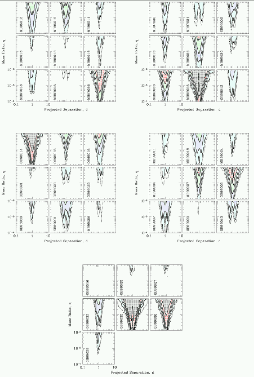
Figure 8: Black lines are contours of constant detection efficiency, $\epsilon(d,q)$, shown for projected separations $d$ between the primary and companion in units of the Einstein ring radius, of $-1<\log{(d)}\leq 1$, and mass ratios between the primary and companion, $q$, of $-2>\log(q)>-4$. Contours mark $\epsilon=1\%$(outer contour; dotted), $5\%$, $25\%$, $50\%$, $75\%$, and $95\%$ (inner contour). Each panel is for a separate event; the abbreviated event name is indicated in each panel. The “wiggly” nature of the outer contours apparent in some events is an artifact of the $(d,q)$ sampling and the plotting routine. Point sources have been assumed here.

The detection efficiency $\epsilon_{i}(d,q)$ is the probability that a companion with mass ratio $q$ and projected separation $d$ would produce a detectable deviation (in the sense of $\Delta\chi^{2}\leq-\Delta\chi^{2}_{\rm thresh}$) in the observed light curve of event $i$. Figure 8 shows $\epsilon_{i}(d,q)$ for our fiducial threshold $\Delta\chi^{2}_{\rm thresh}=60$ and all our events in the parameter range we searched for companions, $0.1\leq d\leq 10$ and $10^{-4}\leq q\leq 10^{-2}$.

We have plotted $\epsilon$ as a function of $\log{d}$, which clearly reveals the $d\rightarrow d^{-1}$ symmetry inherent in planetary perturbations (Griest & Safizadeh 1998; Dominik 1999b). For low magnification events ($u_{0}\geq 0.1$), the efficiency exhibits a “two-pronged” structure as a function of $d$, such that the efficiency has two distinct maxima, one at $d_{\rm\epsilon,max}<1$ and one at $d^{-1}_{\rm\epsilon,max}$, and a local minimum at $d=1$. The approximate locations of these maxima can be found by determining the separations at which the perturbation due to the planetary caustic occurs at the peak of the light curve,

$$d^{\pm 1}_{\rm\epsilon,max}\approx{1\over 2}u_{0}\mp{1\over 2}\sqrt{u_{0}^{2}+4}.$$ (22)

For planetary separations $d_{\rm\epsilon,max}<d<d^{-1}_{\rm\epsilon,max}$, the caustics produced by the companion are within a radius $u_{0}$ of the primary lens, and are thus not well probed by the event. For high magnification events, $\epsilon$ is maximized near $d=1$. This is not only a consequence of equation (22), but also because the central caustic is being probed by the event. As expected, the detection efficiency to companions with any $q$ and $d\lesssim 0.2$ or $d\gtrsim 5$ is negligible for nearly all events.

Of the 43 events, $13$ have very little detection efficiency: for these events, $\epsilon(d,q)$ is larger than 5% for only the most massive companions, and never gets larger that 25%. For the most part, these low efficiencies are due to poorly constrained $u_{0}$. Eight events, notably all high-magnification events, have excellent sensitivity to companions and exhibit $\epsilon(d,q)>95\%$ for a substantial region in the $(d,q)$ plane. Our resultant upper limits on small mass ratio $q\lesssim 10^{-3}$ companions (§8) are dominated by these 8 events. For the remainder of the events, the efficiency is substantial ($\gtrsim 25\%$) for some regions of parameter space. These events contribute significantly to the upper limits for mass ratios $q\gtrsim 10^{-3}$.

In Figure 9, we show the efficiency averaged over the lensing zone (where the detection efficiency is the highest),

$${\epsilon}_{{\rm LZ},i}(q)\equiv\int_{0.6}^{1.6}\epsilon_{i}(d,q)~{}{\rm d}d~{},$$ (23)

as a function of the logarithm of the mass ratio. For a model in which companions have projected separations $d$ distributed uniformly in the lensing zone, ${\epsilon}_{{\rm LZ},i}(q)$ is the probability that a planet of mass ratio $q$ would have been detected in light curve $i$. Also shown is ${\epsilon}_{{\rm LZ},i}$ for a detection threshold of $\Delta\chi^{2}_{\rm thresh}=100$. For this more conservative threshold, the efficiencies are $5-40\%$ lower, though the threshold level is most important where the efficiency is smallest.

7 Finite Source Effects

The results in §6.3 and §6.4 were derived under the implicit assumption that the source stars of the microlensing events could be treated as point-like. Numerous authors have discussed the effect of the finite size of the source on the deviation from the PSPL curve caused by planetary companions (Bennett & Rhie 1996; Gaudi & Gould 1997; Griest & Safizadeh 1998; Gaudi & Sackett 2000; Vermaak 2000). Finite sources smooth out the discontinuous jumps in magnification that occur when the source crosses a caustic curve, and generally lower the amplitude but increase the duration of planetary perturbation. Finite sources also increase the area of influence of the planet in the Einstein ring. Thus finite sources have a competing influence on the detection efficiency: significant point source deviations can be suppressed below the detection threshold, while trajectories for which the limb of the source grazes a high-magnification area can give rise to detectable perturbations when none would have occurred for a point-source. Which effect dominates depends on many factors, including the size of the source relative to the regions of significant deviation from the single-lens form, the photometric precision, and the sampling rate. For large sources and small mass ratios, finite source effects can significantly alter the detection efficiency (Gaudi & Sackett 2000). Since in principle the results presented in §§6.3 and 6.4 could be seriously compromised by ignoring these effects, we evaluate the magnitude of the finite source effect explicitly.

In order to access the magnitude of the finite source effect, we must estimate the angular radius of the source in units of $\theta_{\rm E}$,

$$\rho_{*}={{\theta_{*}}\over{\theta_{\rm E}}}={{\theta_{*}}\over{\mu_{\rm rel}{t_{\rm E}}}}\simeq 0.02\left(\theta_{*}\over 6~{}\mu{\rm as}\right)\left({\mu_{\rm rel}}\over{12.5~{}{\rm km}\,{\rm s}^{-1}{\rm kpc}^{-1}}\right)^{-1}\left({{t_{\rm E}}\over 40~{}{\rm days}}\right)^{-1},$$ (24)

where $\theta_{*}=6~{}\mu{\rm as}$ for a clump giant at $8~{}{\rm kpc}$. For deviations arising from the planetary caustic, finite source effects become important when $\theta_{*}$ is of order or smaller the planetary Einstein ring radius, $\theta_{\rm p}$, i.e, when

$$\rho_{*}\gtrsim\sqrt{q}\qquad{\rm(Planetary~{}Caustics)}.$$ (25)

The size of the central caustic is $u_{\rm c}\sim qd(d-1)^{-2}$ (Griest & Safizadeh 1998). Thus finite sources will affect the magnification due to the central caustic when $\rho_{*}\gtrsim qd(d-1)^{-2}$. However, in order for the central caustic to be probed at all, the event must have an impact parameter $u_{0}\lesssim u_{\rm c}$. Thus finite source will affect deviations arising from the central caustic if

$$\rho_{*}\gtrsim u_{0}\qquad{\rm(Central~{}Caustic)}.$$ (26)

The difficulty in assessing the effect of finite sources on the detection efficiency lies not in evaluating the effect for a given $\rho_{*}$, but rather in determining the appropriate $\rho_{*}$ for a given event. This is clear from equation (24): of the three parameters that determine $\rho_{*}$, ${t_{\rm E}}$ is known from the PSPL fit, $\theta_{*}$ can be estimated based on the color and magnitude of the source, but $\mu_{\rm rel}$ is unknown. Gaudi & Sackett (2000) suggested several possible methods of dealing with this difficulty. The simplest is to assume for all events a proper motion equal to the mean proper motion $\left<\mu_{\rm rel}\right>$, adopting the $\rho_{*}$ given by equation (24) with $\mu_{\rm rel}=\left<\mu_{\rm rel}\right>$. A more accurate, but also more complicated and time-consuming, method is to integrate over a distribution of $\mu_{\rm rel}$ given by a Galactic model; this would imply calculation of finite source effects for many different values of $\rho_{*}$. Here we adopt the first approach and determine $\rho_{*}$ assuming $\mu_{\rm rel}=\left<\mu_{\rm rel}\right>=12.5~{}{\rm km}\,{\rm s}^{-1}{\rm kpc}^{-1}$. This value of $\left<\mu_{\rm rel}\right>$ is a factor of two lower than the expected mean relative proper motion for all lenses toward the bulge (Han & Gould 1995), and reflects the fact that our median ${t_{\rm E}}$ is a factor of two larger than the median of all microlensing events toward the bulge and our belief that the larger time scales reflect the fact that we are preferentially selecting slower (rather than more massive or closer) lenses. We justify this assertion in §9. To the extent that the masses and distances of the lenses contribute somewhat to this larger median time scale, our adopted value of $\left<\mu_{\rm rel}\right>$ is likely an overestimate. Therefore, the resulting values of $\rho_{*}$ are likely overestimates, so that we are conservatively computing upper limits to the effect of the finite source sizes on our conclusions.

7.1 Estimating the Source Sizes

The angular size $\theta_{*}$ of a given source can be estimated from its dereddened $(V-I)_{0}$ color and magnitude $I_{0}$. From the PSPL fits to the $I$ and $V$ photometry, we know the $I$ and $V$ fluxes of the sources in instrumental units (see §4). We assume that the dereddened color $(V-I)_{\rm cl,0}$ and magnitude $I_{\rm cl,0}$ of the clump is invariant for all our fields, adopting the determination by Paczyński et al. (1999),

$$(V-I)_{\rm cl,0}=1.114\pm 0.003,\qquad I_{\rm cl,0}=14.43\pm 0.02.$$ (27)

We form instrumental color-magnitude diagrams (CMDs) for each of our fields, and determine the position of the clump in instrumental units by finding the local maximum in the density of sources. The difference between this position and the intrinsic position [eq. (27)] gives the offsets $\Delta(V-I)$ and $\Delta I$ for all the stars in the field (except foreground stars, which have less reddening than the calibrating clump). Note that these offsets include both the calibration from instrumental to true fluxes, and also the correction for the mean reddening of the field. Thus we do not assume a constant redenning law from field to field. We apply these offsets to the instrumental $(V-I)$ and $I$ of our source stars, finally arriving at the $(V-I)_{0}$ and $I_{0}$ for all our sources. These are shown in Figure 10 and listed in Table 4. The error bars on $(V-I)_{0}$ and $I_{0}$ are those derived from modeling uncertainties; we estimate there to be an additional calibration error of $\sim 5\%$ in both $(V-I)_{0}$ and $I_{0}$ based on the typical dispersion of the clump. Note that the majority ($\sim 70\%$) of our sources are giants.

Using these colors and magnitudes, the angular size of the sources are derived using a modified version of the empirical color-surface brightness relation derived by van Belle (1999) and given in Albrow et al. (2000a). The resulting $\theta_{*}$ for all of our sources are shown in Table 4. The average uncertainty in $\theta_{*}$ is ${\cal O}(20\%)$, combining the uncertainty in the color and magnitude of the source due to both modeling and calibration uncertainty and the uncertainty in the underlying van Belle (1999) relation. We do not determine the uncertainty on $\theta_{*}$ for individual sources because the uncertainty in $\rho_{*}$ (the parameter in which we are primarily interested) is dominated by the uncertainty in $\left<\mu_{\rm rel}\right>$. Seven of our events have insufficient $V$-band data to determine the instrumental $(V-I)$ of the source. For these events, we assumed the source to have the median $(V-I)$ of all sources in the field with similar $I$ magnitudes. (For these events, we do not quote uncertainties on $(V-I)_{0}$.) Finally, four events had either no $V$-band data at all, or the position of the clump was impossible to determine from the CMD of the field. For these events, we simply adopt the conservative assumption that the sources are clump giants, with $\theta_{*}=6~{}\mu{\rm as}$.

These estimates of $\theta_{*}$ are used to determine $\rho_{*}$ under the assumption that all events have the same relative proper motion $\left<\mu_{\rm rel}\right>=12.5~{}{\rm km}\,{\rm s}^{-1}{\rm kpc}^{-1}$; these values of $\rho_{*}$ are listed in Table 4. For two events, MACHO 98-BLG-35 and OGLE-1999-BUL-35, the value of $\rho_{*}$ estimated in this way is larger than the fitted $u_{0}$ of the event. In both cases, the derived values of $\rho_{*}$ are ruled out by the fact that, despite dense coverage at the peak, no deviations from the PSPL form are seen, as would be expected if $\rho_{*}>u_{0}$ and the lens was resolving the source (Gould 1994; Nemiroff & Wickramasinghe 1994; Witt & Mao 1994). For these two events, we therefore assume that $\rho_{*}=u_{0}$. In Figure 11, we plot $u_{0}$ versus $\rho_{*}$ for all our events, along with the boundaries where finite source effects become important for both the planetary and central caustics [eqs. (25) and (26)]. For the majority of our events, finite source effects should not alter the results for companions with $q\gtrsim 10^{-3}$, whereas a large fraction of our events should be affected for $q\sim 10^{-4}$.

7.2 Incorporating Finite Sources

In order to incorporate finite sources into the analysis, we repeat the algorithm presented in §6.1 for all events, but fit the events to binary-lens light curves that include the effect of the finite size of the source. Evaluating the finite-source binary-lens magnification for the specific value of $\rho_{*}$ determined for each event is not computationally feasible, as finite source magnifications are quite time consuming to calculate. We therefore adopt a procedure similar to that described in §6.2.4: interpolation between a grid of finite-source binary-lens magnification maps. We choose the same grid spacing and size for $(d,q)$, namely $10^{-4}\leq q\leq 10^{-2}$ at equal intervals of $0.25$ in $\log{q}$, and $0.1\leq d\leq 10$ at $d=0.1,0.2,...,1.0$ and their inverses. For each of these $(d,q)$ pairs, we create finite-source magnification maps for $10^{-4}\leq\rho_{*}\leq 10^{-1}$ at intervals of $1/3$ dex in $\log{\rho_{*}}$. These maps have same the extent and sampling in the source plane as the point source maps (see §6.2.4). We evaluate the finite-source magnification using the Stokes method of integrating over the boundary of the images (Kayser & Schramm 1988; Gould & Gaucherel 1997). Our assumption of uniform sources overestimates the size of the finite source effect relative to limb-darkened sources, and thus is conservative. The grid value of $\rho_{*}$ closest to the value estimated for each source is used to calculate the detection efficiency for that event. We have repeated this process for the next-closest value of $\rho_{*}$ in the grid for all events, and find that there is no appreciable difference in the conclusions.

7.3 Effect of Source Size on Detection Efficiencies

The distribution of $\Delta\chi^{2}_{\rm min}$ for the finite-source binary-lens fits is shown in Figure 7, along with the distribution for the point-source binary-lens fits. For the most part, the two distributions are quite similar. The significance of the best-fit binary-lens model has increased in some cases (e.g. MACHO 98-BLG-35), but all of the events that fall below our detection threshold ($\Delta\chi^{2}_{\rm min}>-60$) in the point-source case also fall below this threshold in the finite source case. We recover the same two anomalies in MACHO 99-BLG-18 and OGLE-1999-BUL-36, but no others. As argued in §6.3, these two anomalies have explanations other than planetary microlensing for their behavior. Thus our conclusions are unchanged: out of a sample of 43 events, we find no viable planet candidates.

The resulting finite-source lensing zone detection efficiencies [eq. (23)] are shown in Figure 9 along with the corresponding point-source efficiencies. We find, in agreement with the expectations in §7.1, that the difference between the point-source and finite-source efficiencies for mass ratios $q\gtrsim 10^{-3}$ is negligible for nearly all events, with the exception of a few events with very large sources ($\rho_{*}\sim 0.1$). Finite source effects begin to become appreciable for $q\lesssim 10^{-3}$. For $q=10^{-4}$, the finite-source detection efficiency is markedly smaller than the point-source efficiency for large sources. The finite size of the sources has no appreciable effect on the detection efficiencies for those mass ratios where we have significant constraints ($q>10^{-4}$), and conversely for those mass ratios where finite source effects are appreciable we have no interesting constraints. Therefore we conclude that, for this sample of events, finite source effects are negligible.

8 Upper Limits on Planetary Companions

The fact that a large fraction of our final sample of 42 microlensing events has significant detection efficiencies to planetary companions — despite the fact that we have detected no viable planetary candidates in these events — suggests that the fraction of primary lenses with planetary companions in our range of sensitivity must be considerably smaller than unity. To quantify the exact limit implied by our data, we combine the individual event efficiencies $\epsilon_{i}(d,q)$ to obtain a statistical upper limit on the fraction of lenses with companions as a function of mass ratio $q$ and projected separation $d$.

Assume that a fraction $f(d,q)$ of primary lenses have planets with parameters $(d,q)$. Averaged over a large number of events, the probability that any single event would harbor such a planet is then also $f(d,q)$. The probability that such a planet would be detected in event $i$ is the detection efficiency, $\epsilon_{i}(d,q)$. Therefore, the probability that any given event has a planet that is detectable with these data is $f(d,q)\epsilon_{i}(d,q)$. The probability that a planet is not detected is $1-f(d,q)\epsilon_{i}(d,q)$. Thus the probability that a sample of $N$ events would result in at least one detection is simply

$$P(d,q)=1-\Pi_{i=1}^{N}\left[1-f(d,q)\epsilon_{i}(d,q)\right].$$ (28)

The 95% confidence level (c.l.) upper limit to $f(d,q)$ implied by such a sample of events is found by setting $P(d,q)=0.05$ and solving for $f(d,q)$. Note that, in the limit of $f\epsilon_{i}\ll 1$, equation (28) reduces to the naive formula,

$$P(d,q)\rightarrow 1-\exp[-N_{\rm exp}(d,q)]\qquad N_{\rm exp}(d,q)=f(d,q)\sum_{i}\epsilon_{i}(d,q).$$ (29)

We have, however, used the exact expression equation (28) to compute excluded fractions $f(d,q)$.

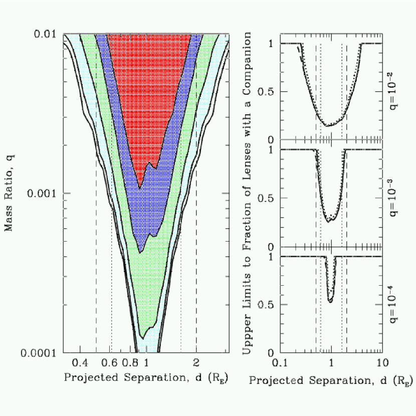
Figure 12: Left Panel: Exclusion contours (95% c.l.) for the fractions of primary lenses with a companion derived from our sample of 43 events, as a function of the mass ratio and projected separation of the companion. Solid black lines show exclusion contours for $f=$75%, 66%, 50%, 33% and 25% (outer to inner). The dotted (dashed) vertical lines indicate the boundaries of the lensing zone (extended lensing zone). Right Panels: Cross sections through the left panel, showing for three different mass ratios the upper limit to the fraction of lenses with a companion as a function of projected separation. The solid line is derived from the point-source efficiencies with a threshold of $\Delta\chi^{2}_{\rm thresh}=60$. The dotted line is derived from the point-source efficiencies with a threshold of $\Delta\chi^{2}_{\rm thresh}=100$. The dashed line is finite-source efficiencies with a threshold of $\Delta\chi^{2}_{\rm thresh}=60$. The dotted vertical lines indicate the boundaries of the lensing zone $0.6\leq d\leq 1.6$. The dashed vertical lines indicate the extended lensing zone, $0.5\leq d\leq 2$.

In Figure 12 we show the 95% c.l. upper limit to $f(d,q)$ as a function of $d,q$ derived from our final sample of 42 events, assuming $\Delta\chi^{2}_{\rm thresh}=60$ and point sources. We conclude that $<28\%$ of lenses have a companion of mass ratio $q\gtrsim 10^{-3}$ and projected separation $d\sim 1$. The hypothesis that more than one-half of the primary lenses have a companion near $d=1$ for the full range of mass ratios $10^{-4}\leq q\leq 10^{-2}$ is excluded with 95% confidence. Also shown in Figure 12 are cross sections of the $(d,q)$ exclusion diagram (95% c.l. upper limits as a function of $d$) for three different mass ratios, namely $q=10^{-2}$, $10^{-3}$, and $10^{-4}$. For these cross sections, we also show the 95% c.l. upper limits derived assuming point sources and $\Delta\chi^{2}_{\rm thresh}=100$, and assuming finite sources and $\Delta\chi^{2}_{\rm thresh}=60$. Clearly finite source effects are negligible in regions where we have interesting constraints.

In Figure 13 we show the 95% c.l. upper limit as a function of $q$ for companions anywhere in the lensing zone $0.6\leq d\leq 1.6$, and anywhere in the “extended” lensing zone, $0.5\leq d\leq 2.0$. Statistically, less than $20\%$ of primaries have a $q=10^{-2}$ mass ratio companion in the lensing zone. For $q=10^{-3}$ companions in the lensing zone, the upper limit is $45\%$.

9 Converting to Planetary Mass and Orbital Separation

The upper limits presented in §8 are the most direct, least model-dependent inferences we can draw from our data. Unfortunately, they are not the most illuminating, for several reasons. First, the nature of primaries around which we limit planets is not specified. Second, our results are quoted in terms of the two natural binary-lens parameters, the mass ratio of the system $q$ and the instantaneous projected separation $d$ of the companion, rather than the more common (and more interesting) parameterization of planetary mass $m_{p}$ and orbital separation $a$.

Unfortunately, it is not possible to directly determine the mass of the primaries, and hence their nature, because the one observable parameter containing information about the lens, the event time scale ${t_{\rm E}}$, is a degenerate combination of the mass, distance, and velocity of the lens [Eqs. 1 and 4]. Only model-dependent inferences about the nature of the primary lenses are possible. The majority of the microlensing events in our sample are likely to be due to bulge stars lensing other bulge stars (Kiraga & Paczyński 1994). Following Gould (2000), we adopt the bulge mass function as measured by Zoccali et al. (2000), and assume a model such that the sources and lenses are distributed as $r^{-2}$, where $r$ is the Galactocentric distance, and have Gaussian velocity distributions with dispersion $\sigma=100~{}{\rm km}\,{\rm s}^{-1}$. This model gives typical parameters for bulge self-lensing events of $\left<M\right>\sim 0.3~{}M_{\odot}$, $\left<\pi_{\rm rel}\right>=40~{}\mu{\rm as}$, and thus $\left<\theta_{\rm E}\right>\sim 320~{}\mu{\rm as}$. For the relative proper motion, this model predicts $\left<\mu_{\rm rel}\right>\sim 25~{}{\rm km}\,{\rm s}^{-1}~{}{\rm kpc}^{-1}$, and thus $\left<{t_{\rm E}}\right>\sim 20~{}{\rm days}$, which is the median time scale found by OGLE for events toward the Galactic bulge (Udalski et al. 2000). Taken at face value, the fact that the median time scale of the events in our sample is a factor of two times larger implies that we are selecting a biased subset of lenses. From equations (1) and (4), this bias could be toward higher mass lenses, slower lenses (smaller $\mu_{\rm rel}$) or closer lenses (larger $\pi_{\rm rel}$), or any combination of these three factors. In fact, as demonstrated by Gould (2000), the majority of the dispersion in the expected distribution of time scales arises from the dispersion in $\mu_{\rm rel}$, not the dispersion in $\pi_{\rm rel}$ or $M$. This implies that we are, for the most part, preferentially selecting slower — rather than more massive or closer — lenses, justifying our assumption of $\left<\mu_{\rm rel}\right>\sim 12.5~{}{\rm km}\,{\rm s}^{-1}~{}{\rm kpc}^{-1}$ for the estimates of $\rho_{*}$ in §7. Thus the typical mass and lens-source relative parallax of the lenses in our sample is likely to be close to those of the complete sample of microlensing events. We therefore adopt $\left<M\right>=0.3~{}M_{\odot}$ and $\left<\pi_{\rm rel}\right>=40~{}\mu{\rm as}$, which for source stars at $D_{\rm S}\sim 8~{}{\rm kpc}$ implies lens distances of $D_{\rm L}\sim 6~{}{\rm kpc}$. In other words, the majority of our primary lenses are $M$ dwarfs in the Galactic bulge.

Some caveats must be noted. Kiraga & Paczyński (1994) estimate that $\sim 20\%$ of events toward the Galactic bulge are due to lensing of bulge stars by disk stars. Of the remaining $\sim 80\%$, Gould (2000) estimates that $\sim 20\%$ are due to remnants (white dwarfs, neutron stars, and black holes). Thus, we would expect $\sim 60\%$ of the events in our sample to be due to normal stars in the Galactic bulge. However, we have no idea which events comprise this 60%. Also, some fraction of the events in our sample are likely members of binary systems with separations that are either too small or (more often) too large to be distinguishable from single lenses. We have no way of determining which events these are, or even what fraction of our events are in such systems. Given our rather small sample of events and the uncertainties in the magnitude of these contaminations, we feel it is not appropriate at this stage to attempt to correct for these effects.

The estimates of $\left<M\right>$ and $\left<\pi_{\rm rel}\right>$ adopted above imply $\left<\theta_{\rm E}\right>=320~{}\mu{\rm as}$ and thus $\left<{r_{\rm E}}\right>=2~{}{\rm AU}$ (for $D_{\rm L}=6~{}{\rm kpc}$). We use these values to convert the upper limits derived in §8 from dimensionless units to physical units, via the relations,

$$m_{p}=\left({q\over 0.003}\right)M_{\rm Jup},\qquad r_{p}=\left({d\over 0.5}\right){\rm AU},$$ (30)

where $r_{\rm P}$ is the analog of $d$ (the instantaneous projected separation) in physical units. To convert from $r_{p}$ to the conventional three-dimensional separation $a$, we must convolve with the distribution function (Gould & Loeb 1992),

$$p(r_{p};a)={r_{p}\over a}\left(1-{r_{p}^{2}\over a^{2}}\right)^{1/2},$$ (31)

which is found by integrating over all random inclinations and orbital phases, assuming circular orbits. Thus the detection efficiency of each event $i$ in the $(a,m_{p})$ plane is,

$$\epsilon_{i}(a,m_{p})=\int_{0}^{a}{\rm d}r_{p}p(r_{p};a)\epsilon_{i}(r_{p},m_{p})$$ (32)

These individual efficiencies $\epsilon_{i}(a,m_{p})$ can now be combined in the same manner as in §8 to derive 95% c.l. upper limits to the fraction $f(a,m_{p})$ of events with companions as a function of the mass $m_{p}$ and separation $a$ of the companion.

In Figure 14 we show the 95% c.l. upper limit to $f(a,m_{p})$ as a function of $a$ and $m_{p}$, assuming $\Delta\chi^{2}_{\rm thresh}=60$ and point sources. This figure is analogous to Figure 12, except that now our upper limits are in terms of the physical variables of the mass of the companion in $M_{\rm Jup}$ and separation of the companion in ${\rm AU}$, and we have identified our primaries as M-dwarfs in the Galactic bulge. In Figure 15 we show the 95% c.l. upper limits to the fraction of lenses with planets in two ranges of orbital separations, $(1.5-4)~{}{\rm AU}$ and $(1-7)~{}{\rm AU}$. Taking our inference about the nature of the primary lenses literally, we conclude that less than 33% of M-dwarfs in the Galactic bulge have Jupiter mass companions between 1.5 and 4$~{}{\rm AU}$. Less than 45% have 3-Jupiter mass companions between 1 and 7$~{}{\rm AU}$. These are the first significant limits on planetary companions to M-dwarfs, and are the primary result of this work.

10 Discussion

The majority of what we know about planetary companions has been gathered from radial velocity surveys of stars in the local neighborhood. However, these surveys have told us very little about planetary companions to M-dwarf primaries, as they have focused on F, G, and K-dwarf and have only recently begun surveying cooler stars. To date, the only M-dwarf with known planetary companions is Gliese 876 (Marcy et al. 1998; Marcy et al. 2001b). Our results therefore place interesting limits in an entirely new region of parameter space. However, this also means that the comparison between our results and those of radial velocity surveys is not entirely straightforward, as we are probing different primaries, and therefore different regimes of star, disk, and planet formation. Furthermore, our primaries are mostly old stars in the bulge, whereas those studied by radial velocity surveys are relatively young (Ford, Rasio, & Sills 1999; Gonzales 1999; Santos, Israelian, & Mayor 2000). Finally, there is evidence that the host stars of local companions have super-solar metallicity (Gonzales 1999; Santos, Israelian, & Mayor 2000), whereas stars in the Galactic bulge likely have solar to sub-solar metallicity. It is not at all clear how these differences between the parent samples we probe will affect the various proposed planet formation mechanisms.

Rather than attempt to interpret our results in the context of these various parameters, which may or may not affect planetary formation, we simply make a direct comparison between our results and those of radial velocity surveys. In Figure 16, we show our 95% c.l. upper limits on the fraction of primaries with a companion as a function of the mass $m_{p}$ and orbital separation axis $a$ of the companion, along with the measured $m_{p}\sin{i}$ and $a$ of those companions detected by radial velocity surveys. For the most part, radial velocity surveys are currently sensitive to companions of smaller $a$ than is microlensing, although there is clearly some overlap. Also shown is the radial-velocity detection limit for a precision of $5~{}{\rm m~{}s^{-1}}$, a primary mass of $0.3~{}M_{\odot}$ (typical of our primaries), and a survey lifetime of 10 years. We also show the astrometric detection limit for $0.3~{}M_{\odot}$ primaries at $10~{}{\rm pc}$ expected for SIM, which should achieve a precision of $10~{}\mu{\rm as}$ and have a survey lifetime of five years.

The results from radial velocity surveys for companions indicate that $f\sim 5\%$ of local F, G, and K-dwarfs have companions between $0\leq a\leq 3~{}{\rm AU}$ (Marcy, Cochran & Mayor 2000). It is interesting to ask how many more events we would need to monitor in order to limit the fraction of primaries with companions to 5% in the range of the separations to which we are sensitive. From equation (29), we find that, for small $f$, $f\propto N_{\rm exp}^{-1}$. Given that our limits are $f\sim 33\%$, we would require $\sim 7$ times more events of similar quality. This number could be significantly reduced if the quality of the alerts could be improved, i.e. if a larger fraction of events we monitor in the future were bright, high-magnification events. This will likely be possible with the next generation OGLE campaign (Udalski et al. 2000).

11 Summary and Conclusion

We have analyzed five years of PLANET photometry of microlensing events toward the Galactic bulge to search for planets. All of the 126 bulge microlensing events for which PLANET has acquired data over the last five years can be subdivided into three categories: events for which the data quality is too poor to determine the nature of the event, events that deviate from the single lens in a way not associated with planetary companions (roughly equal-mass binaries, parallax, finite source, binary source, etc.), and apparently normal point-source point-lens events (PSPL). We find no events in a possible fourth category: events that have short-duration deviations from the single lens light curve that are indicative of the presence of planetary companions to the primary microlenses. This indicates that Jupiter-mass companions to bulge stars with separations of a few AU are not typical.

In order to justify and quantify this conclusion, we imposed strict event selection criterion, and derived a well-defined subset of 43 intensively monitored events which we carefully analyzed for the presence of companions. Using the method of Gaudi & Sackett (2000), we searched for the signatures of planetary companions in these events over a densely sampled, extensive region of parameter space. Specifically, we searched for companions with mass ratios $q$ from $10^{-2}-10^{-4}$ and instantaneous projected separations $d$ in units of the angular Einstein ring radius from $0.1\leq d\leq 10$. Based on an analysis of our photometric uncertainties for constant stars, we required that the difference in $\chi^{2}$ between the best-fit binary lens model and the best-fit single lens model be $<-60$ for a detection candidate. We found two such candidates, events MACHO 99-BLG-18 and OGLE-1999-BUL-36. Analysis of MACHO 99-BLG-18 revealed a significantly better fit with $q\simeq 0.2$, and was eliminated from the sample. OGLE-1999-BUL-36 displays an overall asymmetry that is equally-well (in the sense of $\chi^{2}$) explained by a low-amplitude parallax signal. Since we cannot reliably detect planets from global asymmetries, we explicitly discard this ambiguous anomaly. Thus we find no viable planetary candidates out of our original sample of 43 events.

We then calculated the detection efficiency for our events in $(d,q)$ space. Of our final sample of 42 events (eliminating MACHO 99-BLG-18), 30 have substantial ($>25\%$) efficiency for the detection of companions with $q=10^{-2}$ and separations in the lensing zone $0.6\leq d\leq 1.6$. Had all of the primary lenses harbored such companions, we should have detected a planet in at least $\sim 7$ of them. The fact that we detected no companions implies that this is not the case. By combining our efficiencies, we obtain statistical upper limits on the fraction of lenses with massive planets in the lensing zone. At the 95% confidence level, we find that $<25\%$ of lenses can have a companion in the lensing zone with mass ratio $q=10^{-2}$ .

Using a model of the mass function, spatial distribution, and velocity distribution of stars in the Galactic bulge, we infer that the majority of our lenses are likely due to $M\sim 0.3~{}M_{\odot}$ stars at $6~{}{\rm kpc}$, i.e. M dwarfs in the Galactic bulge. Using this assumption, we convert our upper limits from $(q,d)$ space to mass-orbital separation space. We conclude that less than 33% of M-dwarfs in the Galactic bulge have Jupiter-mass companions between 1.5 and 4$~{}{\rm AU}$, and less than 45% have 3-Jupiter mass companions between 1 and 7$~{}{\rm AU}$. These are the first significant limits on planetary companions to M-dwarfs.

We have also tested the robustness of our conclusions to various assumptions. The effect of the finite size of the source stars was estimated for each event using the color and magnitude of the source and assuming a mean relative proper motion of the lens. We find that the finite source effect becomes important only for mass ratios $q\lesssim 10^{-3}$, where our constraints on companions are already weak. We therefore conclude that finite source effects have a negligible effect on our results. We also tested the effect of changing our detection criterion from $\Delta\chi^{2}_{\rm thresh}=60$ to $\Delta\chi^{2}_{\rm thresh}=100$. As expected, this lowers our sensitivity somewhat, and increases our upper limits by $\lesssim 20\%$, but does not change our conclusions substantially. Finally, we have tested the effect of ignoring parallax asymmetries in the calculation of our detection efficiencies, and find that this changes our limits by substantially less than our statistical uncertainties.

We find that our median event time scale (${t_{\rm E}}=40~{}{\rm days}$) is a factor of two larger than the median time scale for all events toward the Galactic bulge, a selection effect that arises from the manner in which we choose our targets. We argued that this primarily biases our events toward slower, rather than closer or more massive lenses. Therefore, our assertion of a typical lens mass of $0.3~{}M_{\odot}$ is justified.

For the most part our upper limits are for planets with orbital separations that are larger than those currently probed by radial velocity techniques, since the orbital times are longer than the finite survey lifetimes. However, the smallest separations to which we are sensitive overlap with current radial velocity surveys, and as the radial velocity surveys continue, the degree of overlap will increase. Thus one will eventually be able to compare the frequency of companions in the Galactic bulge with that in the solar neighborhood. We estimate, however, that a sample $\sim 7$ times larger than that considered here would be needed to probe fractions as small as those being measured by radial velocity surveys ($\sim 5\%$), assuming assuming that future microlensing observations are of similar quality to those analyzed here. If the number of alerts is increased substantially, however, more care could be taken to choose higher-quality (brighter, higher maximum magnification) events. This would considerably reduce the number of event needed to probe companion fractions of $5\%$.

Our results have implications for theories of planet formation, as the orbital separations we probe may be closer to the sites of planet formation than the small separations at which radial-velocity companions are found, which may be reached via orbital migration. In any case, the limits described here provide fundamental constraints on the frequency and distribution of extrasolar planets orbiting the most common stars in our Galaxy.

Appendix A Excluded Anomalous Events

In §4, we rejected from the analysis 19 anomalous events which we asserted were not caused by planetary (i.e. small mass ratio binary) lenses. Here we list each of these events, and briefly justify why we believe their anomalies to be non-planetary in origin. For those events for which binary-lens fits are available in the literature, we will simply state the fitted mass ratio(s), and refer the reader to the paper; for a large fraction of these events, we rely on the analysis and binary-lens fits of Alcock et al. (2000). One caveat should be noted. It is known (Dominik & Hirshfeld 1996; Dominik 1999a; Albrow et al. 1999b) that binary lens events, even extremely well sampled ones, often have degenerate solutions (Afonso et al. 2000). This is due to intrinsic degeneracies in the binary lens equation (Dominik 1999b). Finding all of these degenerate solutions to an observed light curve is highly non-trivial, due to the extremely sharp variations in $\chi^{2}$ with respect to the canonical parameters, although several methods have been proposed to deal with this difficulty (Di Stefano & Mao 1996; Di Stefano & Perna 1997; Albrow et al. 1999b). It is therefore possible, as Alcock et al. (2000) allow, that not all solutions have been found and thus that some of the events they analyze actually have planetary solutions that they missed. Based simply on examination of the data we find this unlikely, since the deviations from the PSPL form are gross and long duration, contrary to what would be expected from a small mass ratio binary.

For caustic-crossing binary-lens events for which the source is resolved, we can use the following argument to place a lower limit on the mass ratio $q$. The maximum magnification obtained when a source of angular size $\theta_{*}$ crosses a fold caustic is (Schneider, Ehlers, & Falco 1992)

$$A^{\rm cf}_{\rm max}\sim\left(u_{\rm r}\over\theta_{*}\right)^{1/2},$$ (A1)

whereas for a cusp caustic,

$$A^{\rm cc}_{\rm max}\sim\left(u_{\rm r}\over\theta_{*}\right).$$ (A2)

Here $u_{\rm r}$ is a factor that describes the characteristic scale of the caustic. For caustics originating from binary lenses with small $q$, this scale is of order the planetary Einstein ring radius, $\theta_{\rm p}$. Due to possible blending, the observed maximum magnification, $A^{\rm cf}_{\rm max,obs}$ (or $A^{\rm cc}_{\rm max,obs}$), is a lower limit to the true magnification, and by combining eqs. (A1), (1), and (24), we obtain an approximate lower limit on $q$ for a fold caustic crossing:

$$q_{\rm min}\gtrsim 0.01\left({A^{\rm cf}_{\rm max,obs}\over 6}\right)^{4}\left({\theta_{*}\over 1~{}\mu{\rm as}}\right)^{2}\left({\mu_{\rm rel}\over 12.5~{}{\rm km}\,{\rm s}^{-1}~{}{\rm kpc^{-1}}}\right)^{-2}\left({t_{\rm E,obs}\over 40~{}{\rm days}}\right)^{-2},$$ (A3)

and combining eqs. (A2), (1), and (24), we obtain a similar relation for a cusp crossing:

$$q_{\rm min}\gtrsim 0.01\left({A^{\rm cc}_{\rm max,obs}\over 30}\right)^{2}\left({\theta_{*}\over 1~{}\mu{\rm as}}\right)^{2}\left({\mu_{\rm rel}\over 12.5~{}{\rm km}\,{\rm s}^{-1}~{}{\rm kpc^{-1}}}\right)^{-2}\left({t_{\rm E,obs}\over 40~{}{\rm days}}\right)^{-2},$$ (A4)

where $t_{\rm E,obs}$ is the observed (i.e. blended) time scale of the event, which is always a lower limit to the true time scale. Since $q_{\rm min}$ is proportional to $t_{\rm E,obs}$ squared, while $q_{\rm min}$ is proportional to $A^{\rm cf}_{\rm max,obs}$ to the fourth power and $A^{\rm cc}_{\rm max,obs}$ squared, the limits in Eqs. A4 and A3 hold even in the presence of blending. The smallest sources in the Galactic bulge have $\theta_{*}\sim 1~{}\mu{\rm as}$, and the dispersion in $\mu_{\rm rel}$ for bulge-bulge lensing is a factor of $\sim 2$. Thus, an observed fold crossing with $A^{\rm cf}_{\rm max,obs}\gtrsim 10$ is almost certainly due to binary lens with mass ratio $q\geq 0.01$. A cusp crossing with $A^{\rm cc}_{\rm max,obs}\gtrsim 40$ is almost certainly due to a binary with $q\geq 0.01$. In general, for reasonably well-sampled events, a cusp approach can be easily distinguished by eye from caustic crossing events. For disk-disk lensing, for which $\mu_{\rm rel}\sim 5~{}{\rm km}\,{\rm s}^{-1}~{}{\rm kpc^{-1}}$, somewhat smaller mass ratios are allowed; however such events are generally rare.

MACHO 95-BLG-12

Both PLANET (Albrow et al. 1998), and MACHO/GMAN (Alcock et al. 2000) data show a smooth double-peaked event, with both peaks having comparable duration. This morphology suggests a weak binary lens or binary source (Griest & Hu 1992). However, the achromaticity of the event favors a binary-lens interpretation, and we find that a binary-source model provides a poor fit to the PLANET data. We cannot uniquely constrain a binary-lens fit, but Alcock et al. (2000) find a binary-lens fit with mass ratio $q=0.47$. The fact that the peaks are of comparable duration precludes a small mass ratio binary-lens (i.e. planetary) model.

MACHO 96-BLG-04

MACHO/GMAN data show two nearly equal-duration deviations separated by $\sim 500~{}{\rm days}$ (Alcock et al. 2000). Both deviations are separately well-fit by a standard PSPL model, suggesting a widely-separated binary-source or binary-lens (Di Stefano & Mao 1996). Alcock et al. (2000) find $q=0.88$ for their binary-lens fit. Regardless of the interpretation, the PLANET data on this event would not have passed our second cut, due to insufficient data.

MACHO 97-BLG-28

We find only one viable model that fits our data for this event (Albrow et al. 1999a), with $q=0.23$. Alcock et al. (2000) find a similar binary-lens model fit for their dataset, with $q=0.21$.

MACHO 97-BLG-41

Our data for this peculiar event is well fit by a rotating binary-lens model with mass ratio $q=0.34$ (Albrow et al. 2000a). Bennett et al. (1999) favor the interpretation that this event is a planet orbiting a binary lens. Our data are clearly inconsistent with their particular fit, although this does not preclude the possibility that some fit of this nature would explain our data. Regardless of the interpretation, this event is rejected because of the presence of the binary.

MACHO 98-BLG-6

This is a long-timescale ($>100~{}{\rm days}$) event which shows global deviations from the PSPL form indicative of parallax.

MACHO 98-BLG-12

MACHO/GMAN data indicate that this event likely underwent four caustic crossings, with each pair of crossings separated by $\sim 40~{}{\rm days}$ (Alcock et al. 2000). The MACHO/GMAN data have poor coverage of the first set of caustic crossings, but constrain the amount of time that the source was between the second set of crossings to be ${{}_{<}\atop{}^{{}^{\sim}}}3~{}{\rm days}$. Due to its short duration, one might suppose that the second set of crossings was due to a planetary caustic. However, the first set of caustic crossings, combined with the fact that the event exhibits a rise toward the second set of crossings, makes this interpretation impossible. Indeed, Alcock et al. (2000) find that the event is well fit by an intermediate-topology binary lens with $q=0.68$. PLANET acquired a few data points immediately after the second crossing, and data immediately after the fourth crossing continuing until the end of the event. Due to the fact that the PLANET data did not probe any of the caustic structures, we find that our dataset is reasonably well fit by a PSPL model. However, our data alone fail our $\delta u_{0}/u_{0}$ cut.

MACHO 98-BLG-14

Both the MACHO/GMAN dataset (Alcock et al. 2000) and the PLANET dataset show a highly asymmetric light curve with a “shoulder” and then a peak. Such a morphology is indicative of a weakly-perturbed binary-lens event, and as such is prone to degeneracies. In fact Alcock et al. (2000) find two fits, one with mass ratio $q=0.09$ and the other with $q=0.22$. However, the event deviates from the PSPL form for a large fraction ($\sim 40\%$) of its apparent duration, making a planetary interpretation unlikely. We performed a systematic search of binary-lens fits to this event, using our data and the MACHO data. We recover the fits reported by (Alcock et al. 2000), along with a few other fits of similar significance. The best-fit binary with $q<0.01$ is ruled out at the $\Delta\chi^{2}=50$ level.

MACHO 98-BLG-16

MACHO/GMAN data show a short duration peak, followed by an abrupt rise and a plateau at magnification $\sim 10$ that lasts $\sim 8~{}{\rm days}$. Following the plateau, the event returned to magnification $\sim 2$ (Alcock et al. 2000). Although the coverage is poorer, PLANET data qualitatively confirm this behavior. This morphology is consistent with a caustic-crossing binary lens event in which the short-time scale peak is due to a cusp approach, followed by a pair of fold caustic crossings with the usual intra-caustic plateau. MACHO/GMAN data near the peak of the first fold caustic crossing have $A^{\rm cf}_{\rm max,obs}\sim 20$, and thus constrain the event to be non-planetary by equation (A3). Indeed, Alcock et al. (2000) find a binary-lens fit with $q=0.68$.

MACHO 98-BLG-42

Alcock et al. (2000) find $q=0.33$. PLANET data cover the second half of the event, including the falling side of a second caustic crossing. Our data of the second crossing show no evidence of a cusp approach, favoring a pure fold caustic crossing. The data near the peak of this fold crossing have $A^{\rm cf}_{\rm max,obs}\sim 40$; therefore the event must be non-planetary in origin [eq.(A3)].

OGLE-1998-BUL-28

This event displays a double-peaked structure indicative of a weak binary-lens or binary source. This is seen in both OGLE and PLANET data for the event. Using the combined dataset, we find the best-fit binary-lens model has $q=0.34$ and $b=0.42$. Normalizing the errors to this model, the best model in the range $q=10^{-4}-10^{-2}$ has $\Delta\chi^{2}\sim 19$, and thus is excluded.

OGLE-1998-BUL-29

PLANET data for this high-magnification ($A_{\rm max}\sim 50$) event show deviations from the PSPL form near the peak of the event that are indicative of source resolution effects. We find that a point-lens finite-source model fits the data quite well. In contrast, we find that the best-fit point-source planetary model in the range $q=10^{-4}-10^{-2}$ is a significantly worse fit ($\Delta\chi^{2}>100$).

MACHO 99-BLG-8

Similar to MACHO 98-BLG-6, this long-time scale event shows severe parallax effects. We also find short time scale variability in the source.

MACHO 99-BLG-22

Although the PLANET, MACHO, and OGLE data show no obvious anomalous behavior, our PSPL fit to the combined datasets yielded a time scale of ${t_{\rm E}}\sim 900~{}{\rm days}$, leading us to suspect parallax effects might be present. In fact, we find that a fit with parallax improves $\chi^{2}$ significantly, and results in a much more reasonable time scale. This interpretation is confirmed by the analysis of Mao et al. (2001). This event is excluded since our algorithm does not currently allow the search for planets atop other microlensing anomalies.

MACHO 99-BLG-25

MACHO data for MACHO 99-BLG-25 show a clear deviation from PSPL at early times, in the form a smaller amplitude, but nearly equal duration peak occurring before PLANET began monitoring the event. The fact that both peaks are of similar duration suggests that this event is likely due to a binary source, and exclude the possibility that it is due to a planet. Our data only cover the rise and fall of the second peak and are perfectly consistent with a PSPL model. In fact, we find that this event does not have a significant planetary signal, nor does it have a large detection efficiency to planetary companions. Therefore excluding this event has no significant impact on our conclusions.

MACHO 99-BLG-47

PLANET data show a departure from the PSPL form lasting $\sim 3~{}{\rm days}$ near the peak. Detailed analysis of this event shows that the deviation is caused by a small separation binary with $q\sim 0.4$ (Albrow et al. 2001c).

MACHO 99-BLG-57

MACHO data show a large, long duration deviation from the PSPL form that is likely due to a binary-source or binary-lens. PLANET has very little data on this event, and so cannot confirm or clarify the nature of this anomaly.

OGLE-1999-BUL-11

A caustic-crossing binary lens; PLANET data resolve the second crossing. The full dataset indicate a pair of pure fold caustic crossings. The second (fold) crossing has $A^{\rm cf}_{\rm max,obs}\sim 10$; thus the event must be non-planetary in origin [eq.(A3)].

OGLE-1999-BUL-23

We find only one viable fit to this event, with $q=0.39$ (Albrow et al. 2001a).

OGLE-1999-BUL-25

PLANET data show a large positive deviation lasting $<1~{}{\rm day}$ superposed atop an extremely noisy light curve. As we see a sharp change in the slope of the light curve immediately after this deviation, we conclude that it is due a caustic crossing of some kind. It is not clear whether this deviation is due to a cusp or fold caustic crossing. We therefore conservatively assume that it is due to a cusp. The observed magnification at the peak of this deviation is $A^{\rm cc}_{\rm max,obs}\sim 40$, and thus from equation (A4), the deviation cannot be due to planet.

OGLE-1999-BUL-42

OGLE data indicate a double peaked structure to the light curve, which is likely due to an nearly equal-mass binary lens or a binary source. The PLANET data cover the rise and fall of the second peak, and are consistent with a single lens model. Regardless of the nature of the anomaly, the light curve would not pass the cut on the uncertainty in $u_{0}$.

Appendix B OGLE-1999-BUL-36 and Parallax Contamination

Figure 17 shows the PLANET and OGLE data for event OGLE-1999-BUL-36, binned into 1 day intervals, along with the best-fit single-lens, binary-lens, and parallax asymmetry models to the unbinned data. The difference in $\chi^{2}$ between the binary-lens and parallax models is $4$ (with the binary-lens model giving the worse fit); both models are favored over the PSPL model by $\Delta\chi^{2}\sim 80$. The best-fit binary lens model has $q=0.0028$, $d=0.60$, and $\alpha=1^{\circ}$. We also find fits for other mass ratios and separations that are nearly as good. The parallax asymmetry fit (see Gould, Miralda-Escudé, & Bahcall 1994 for the exact form) yields a measurement of the asymmetry factor, $\kappa$, given by,

$$\kappa=\Omega_{\oplus}{v_{\oplus}\over\tilde{v}}\sin\lambda\sin\phi,$$ (B1)

where $\tilde{v}=v(D_{\rm S}/D_{\rm LS})$ is the transverse velocity of the lens projected on the observer plane, $\Omega_{\oplus}=2\pi~{}{\rm yr}^{-1}$, $v_{\oplus}\simeq 30~{}{\rm km}\,{\rm s}^{-1}$ is the speed of the Earth, and $\lambda$ is the angle between the source and Sun at the time of maximum magnification. In the case of OGLE-1999-BUL-36, $\sin\lambda\sim 0.6$. We find $\kappa=0.0021\pm 0.0001$, which implies,

$${\tilde{v}\over\sin{\phi}}=143\pm 7~{}{\rm km}\,{\rm s}^{-1}.$$ (B2)

Combining this constraint with ${t_{\rm E}}$, we find an upper limit to the mass of the lens as a function of the distance to the lens,

$$M\lesssim 0.1~{}M_{\odot}{{1-x}\over x},$$ (B3)

where $x=D_{\rm L}/D_{\rm S}$. Thus, if the parallax interpretation is correct, the lens must be closer to us than $\sim 4~{}{\rm kpc}$ in order to be above the hydrogen burning limit.

The primary lesson learned from the analysis of OGLE-1999-BUL-36 is that we cannot robustly detect planetary companions based on global asymmetries, since they cannot be distinguished from low-level parallax. However, when calculating our detection efficiencies (§6.4), we excluded all deviations that produced $\Delta\chi^{2}>60$, including asymmetries. Therefore, our efficiencies are overestimated. In order to estimate by how much, we choose a well-sampled, high-quality event, OGLE-1998-BUL-14, that contains data on both rising and falling sides. We repeat the algorithm in §6.1 to calculate the efficiency of this event but simultaneously fit for both the binary-lens magnification and parallax asymmetry. This procedure removes all detections based on asymmetry alone. In Figure 18 we show the detection efficiency both with and without excluding such detections. The difference is quite small, a few percent, because a very small range of angles produce deviations consistent with asymmetries. The majority of our events have sampling and photometric accuracy that is poorer than OGLE-1998-BUL-14, in which case they will be less sensitive to asymmetries. We therefore conclude that this effect is negligible.

Official Alert Name	Abbreviated Name	Status	Notes
MACHO 95-BLG-10	MB95010	Cut	Uncertainty in $u_{0}$
MACHO 95-BLG-12	MB95012	Cut	Binary
MACHO 95-BLG-13	MB95013	Passed	–
MACHO 95-BLG-17	MB95017	Cut	Uncertainty in $u_{0}$
MACHO 95-BLG-18	MB95018	Cut	Uncertainty in $u_{0}$
MACHO 95-BLG-19	MB95019	Passed	–
MACHO 95-BLG-21	MB95021	Cut	Insufficient Data
MACHO 95-BLG-24	MB95024	Cut	Insufficient Data
MACHO 95-BLG-25	MB95025	Cut	Insufficient Data
MACHO 95-BLG-30	MB95030	Cut	Uncertainty in $u_{0}$
OGLE-1995-BUL-04	OB95004	Cut	Uncertainty in $u_{0}$
MACHO 96-BLG-1	MB96001	Cut	Insufficient Data
MACHO 96-BLG-4	MB96004	Cut	Binary
MACHO 96-BLG-5	MB96005	Cut	Uncertainty in $u_{0}$
MACHO 96-BLG-6	MB96006	Cut	Uncertainty in $u_{0}$
MACHO 96-BLG-7	MB96007	Cut	Uncertainty in $u_{0}$
MACHO 96-BLG-8	MB96008	Cut	Uncertainty in $u_{0}$
MACHO 96-BLG-9	MB96009	Cut	Uncertainty in $u_{0}$
MACHO 96-BLG-10	MB96010	Cut	Uncertainty in $u_{0}$
MACHO 96-BLG-11	MB96011	Passed	–
MACHO 96-BLG-12	MB96012	Cut	Uncertainty in $u_{0}$
MACHO 96-BLG-13	MB96013	Cut	Insufficient Data
MACHO 96-BLG-14	MB96014	Cut	Uncertainty in $u_{0}$
MACHO 96-BLG-15	MB96015	Cut	Insufficient Data
MACHO 96-BLG-16	MB96016	Passed	–
MACHO 96-BLG-17	MB96017	Cut	Insufficient Data
MACHO 96-BLG-18	MB96018	Passed	–
MACHO 96-BLG-19	MB96019	Passed	–
MACHO 96-BLG-20	MB96020	Cut	Uncertainty in $u_{0}$
MACHO 96-BLG-21	MB96021	Cut	Uncertainty in $u_{0}$
MACHO 96-BLG-23	MB96023	Cut	Uncertainty in $u_{0}$
MACHO 96-BLG-24	MB96024	Cut	Insufficient Data
MACHO 96-BLG-25	MB96025	Cut	Uncertainty in $u_{0}$
MACHO 96-BLG-26	MB96026	Cut	Uncertainty in $u_{0}$
MACHO 96-BLG-27	MB96027	Cut	Insufficient Data

Table 1: All Events from 1995-1999 with PLANET data.

Official Alert Name	Abbreviated Name	Status	Notes
MACHO 97-BLG-10	MB97010	Cut	Insufficient Data
MACHO 97-BLG-18	MB97018	Passed	–
MACHO 97-BLG-25	MB97025	Passed	–
MACHO 97-BLG-26	MB97026	Passed	–
MACHO 97-BLG-28	MB97028	Cut	Binary
MACHO 97-BLG-30	MB97030	Passed	–
MACHO 97-BLG-31	MB97031	Passed	–
MACHO 97-BLG-36	MB97036	Cut	Insufficient Data
MACHO 97-BLG-37	MB97037	Cut	Uncertainty in $u_{0}$
MACHO 97-BLG-41	MB97041	Cut	Binary
MACHO 97-BLG-49	MB97049	Cut	Insufficient Data
MACHO 97-BLG-50	MB97050	Cut	Uncertainty in $u_{0}$
MACHO 97-BLG-52	MB97052	Cut	Uncertainty in $u_{0}$
MACHO 97-BLG-54	MB97054	Cut	Insufficient Data
MACHO 97-BLG-56	MB97056	Cut	Insufficient Data
MACHO 97-BLG-58	MB97058	Cut	Insufficient Data
MACHO 97-BLG-59	MB97059	Cut	Insufficient Data

Table 1: Continued

Official Alert Name	Abbreviated Name	Status	Notes
EROS BLG-1998-2	EB98002	Passed	–
EROS BLG-1998-4	EB98004	Cut	Insufficient Data
MACHO 98-BLG-1	MB98001	Cut	Insufficient Data
MACHO 98-BLG-5	MB98005	Cut	Insufficient Data
MACHO 98-BLG-6	MB98006	Cut	Parallax
MACHO 98-BLG-12	MB98005	Cut	Binary
MACHO 98-BLG-13	MB98013	Passed	–
MACHO 98-BLG-14	MB98013	Cut	Binary
MACHO 98-BLG-16	MB98016	Cut	Binary
MACHO 98-BLG-17	MB98017	Cut	Uncertainty in $u_{0}$
MACHO 98-BLG-18	MB98018	Cut	Uncertainty in $u_{0}$
MACHO 98-BLG-19	MB98019	Cut	Insufficient Data
MACHO 98-BLG-22	MB98022	Cut	Insufficient Data
MACHO 98-BLG-24	MB98024	Cut	Insufficient Data
MACHO 98-BLG-26	MB98026	Passed	–
MACHO 98-BLG-27	MB98027	Cut	Uncertainty in $u_{0}$
MACHO 98-BLG-28	MB98028	Cut	Insufficient Data
MACHO 98-BLG-30	MB98030	Passed	–
MACHO 98-BLG-31	MB98031	Cut	Insufficient Data
MACHO 98-BLG-33	MB98033	Passed	–
MACHO 98-BLG-35	MB98035	Passed	–
MACHO 98-BLG-37	MB98037	Cut	Uncertainty in $u_{0}$
MACHO 98-BLG-38	MB98038	Cut	Uncertainty in $u_{0}$
MACHO 98-BLG-39	MB98039	Cut	Uncertainty in $u_{0}$
MACHO 98-BLG-40	MB98040	Cut	Uncertainty in $u_{0}$
MACHO 98-BLG-42	MB98042	Cut	Binary
$*$OGLE-1998-BUL-13	OB98013	Passed	–
$*$OGLE-1998-BUL-14	OB98014	Passed	–
$*$OGLE-1998-BUL-15	OB98015	Passed	–
$*$OGLE-1998-BUL-18	OB98018	Passed	–
$*$OGLE-1998-BUL-20	OB98020	Cut	Insufficient Data
$*$OGLE-1998-BUL-21	OB98021	Passed	–
$*$OGLE-1998-BUL-23	OB98023	Passed	–
$*$OGLE-1998-BUL-25	OB98025	Passed	–
$*$OGLE-1998-BUL-26	OB98026	Cut	Uncertainty in $u_{0}$
$*$OGLE-1998-BUL-27	OB98027	Cut	Uncertainty in $u_{0}$
$*$OGLE-1998-BUL-28	OB98028	Cut	Binary
$*$OGLE-1998-BUL-29	OB98029	Cut	Finite Source
$*$OGLE-1998-BUL-30	OB98030	Passed	–

Table 1: Continued

Official Alert Name	Abbreviated Name	Status	Notes
EROS BLG-1999-1	EB99001	Passed	–
EROS BLG-1999-2	EB99002	Cut	Insufficient Data
$*$MACHO 99-BLG-6	MB99006	Passed	–
$*$MACHO 99-BLG-8	MB99008	Cut	Parallax
$*$MACHO 99-BLG-11	MB99011	Passed	–
$*$MACHO 99-BLG-18	MB99018	Passed	Deviation near peak
$*$MACHO 99-BLG-22	MB99022	Cut	Parallax
$*$MACHO 99-BLG-24	MB99024	Passed	–
$*$MACHO 99-BLG-25	MB99025	Cut	Binary Source?
$*$MACHO 99-BLG-34	MB99034	Passed	–
$*$MACHO 99-BLG-37	MB99037	Passed	–
$*$MACHO 99-BLG-42	MB99042	Cut	Insufficient Data
$*$MACHO 99-BLG-45	MB99045	Cut	Insufficient Data
$*$MACHO 99-BLG-47	MB99047	Cut	Binary
$*$MACHO 99-BLG-57	MB99057	Cut	Binary Lens/Binary Source?
$*$OGLE-1998-BUL-5	OB99005	Passed	–
$*$OGLE-1999-BUL-7	OB99007	Passed	–
$*$OGLE-1999-BUL-8	OB99008	Passed	–
$*$OGLE-1999-BUL-11	OB99011	Cut	Binary
$*$OGLE-1999-BUL-13	OB99013	Passed	–
$*$OGLE-1999-BUL-14	OB99014	Cut	Uncertainty in $u_{0}$
$*$OGLE-1999-BUL-16	OB99016	Passed	–
$*$OGLE-1999-BUL-17	OB99017	Cut	Insufficient Data
$*$OGLE-1999-BUL-19	OB99019	Cut	Insufficient Data
$*$OGLE-1999-BUL-22	OB99022	Passed	–
$*$OGLE-1999-BUL-23	OB99023	Cut	Binary
$*$OGLE-1999-BUL-25	OB99025	Cut	Binary
$*$OGLE-1999-BUL-27	OB99027	Passed	–
$*$OGLE-1999-BUL-33	OB99033	Passed	–
$*$OGLE-1999-BUL-35	OB99035	Passed	–
$*$OGLE-1999-BUL-36	OB99036	Passed	Global Asymmetry
$*$OGLE-1999-BUL-39	OB99039	Passed	–
$*$OGLE-1999-BUL-40	OB99040	Cut	Insufficient Data
$*$OGLE-1999-BUL-42	OB99042	Cut	Uncertainty in $u_{0}$
$*$OGLE-1999-BUL-43	OB99043	Cut	Insufficient Data

Table 1: Continued

Event Name	$t_{0}$	$t_{E}$	$u_{0}$	$\delta u_{0}/u_{0}$
	(HJD-2450000)	(days)		(%)
MB95013	$-$101.169 $\pm$ 0.034	80.85 $\pm$ 2.71	0.245 $\pm$ 0.010	3
MB95019	$-$93.573 $\pm$ 0.030	38.22 $\pm$ 6.41	0.189 $\pm$ 0.035	18
MB96011	241.405 $\pm$ 0.058	10.59 $\pm$ 1.66	0.223 $\pm$ 0.046	20
MB96016	259.777 $\pm$ 0.265	57.19 $\pm$ 24.70	0.094 $\pm$ 0.046	48
MB96018	259.391 $\pm$ 0.041	7.07 $\pm$ 1.98	0.132 $\pm$ 0.045	34
MB96019	266.944 $\pm$ 0.129	12.03 $\pm$ 1.95	0.292 $\pm$ 0.065	22
MB97018	609.529 $\pm$ 0.497	100.19 $\pm$ 30.14	0.329 $\pm$ 0.134	40
MB97025	598.011 $\pm$ 1.423	20.75 $\pm$ 6.18	0.342 $\pm$ 0.164	47
MB97026	636.624 $\pm$ 0.007	68.17 $\pm$ 2.70	0.113 $\pm$ 0.005	4
MB97030	601.243 $\pm$ 0.050	23.43 $\pm$ 2.69	0.080 $\pm$ 0.011	13
MB97031	593.439 $\pm$ 1.772	41.05 $\pm$ 4.33	0.645 $\pm$ 0.128	19
EB98002	964.024 $\pm$ 0.041	23.97 $\pm$ 1.12	0.335 $\pm$ 0.021	6
MB98013	930.529 $\pm$ 0.027	18.24 $\pm$ 3.47	0.063 $\pm$ 0.014	21
MB98026	986.377 $\pm$ 0.022	33.73 $\pm$ 1.15	0.229 $\pm$ 0.009	4
MB98030	992.117 $\pm$ 0.093	26.95 $\pm$ 8.95	0.285 $\pm$ 0.111	38
MB98033	990.463 $\pm$ 0.002	7.33 $\pm$ 0.15	0.148 $\pm$ 0.004	2
MB98035	999.157 $\pm$ 0.001	27.46 $\pm$ 1.17	0.0100 $\pm$ 0.0005	4
$*$OB98013	945.081 $\pm$ 0.157	55.30 $\pm$ 3.03	0.299 $\pm$ 0.022	7
$*$OB98014	956.033 $\pm$ 0.005	41.52 $\pm$ 0.78	0.061 $\pm$ 0.001	2
$*$OB98015	943.840 $\pm$ 0.007	52.24 $\pm$ 10.72	0.006 $\pm$ 0.001	24
$*$OB98018	971.078 $\pm$ 0.006	7.64 $\pm$ 0.16	0.208 $\pm$ 0.006	2
$*$OB98021	992.190 $\pm$ 0.410	26.64 $\pm$ 5.75	0.419 $\pm$ 0.135	32
$*$OB98023	998.735 $\pm$ 0.151	18.60 $\pm$ 2.92	0.514 $\pm$ 0.107	20
$*$OB98025	1041.701 $\pm$ 0.250	50.49 $\pm$ 7.88	0.298 $\pm$ 0.063	21
$*$OB98030	1043.417 $\pm$ 0.069	54.26 $\pm$ 21.85	0.049 $\pm$ 0.021	42
EB99001	1415.023 $\pm$ 0.021	20.19 $\pm$ 1.39	0.517 $\pm$ 0.045	8
$*$MB99006	1247.546 $\pm$ 0.130	27.24 $\pm$ 1.69	0.150 $\pm$ 0.017	11
$*$MB99011	1286.711 $\pm$ 0.117	45.17 $\pm$ 2.42	0.191 $\pm$ 0.015	7
$*$MB99018	1301.897 $\pm$ 0.019	21.69 $\pm$ 0.52	0.462 $\pm$ 0.016	3
$*$MB99024	1304.710 $\pm$ 0.192	59.74 $\pm$ 7.37	0.151 $\pm$ 0.024	15
$*$MB99034	1326.699 $\pm$ 0.152	7.04 $\pm$ 0.59	0.332 $\pm$ 0.049	14
$*$MB99037	1354.220 $\pm$ 0.031	63.59 $\pm$ 5.63	0.076 $\pm$ 0.007	9

Table 2: Point-Source Point-Lens Fit Parameters for the final event sample.

Event Name	$t_{0}$	$t_{E}$	$u_{0}$	$\delta u_{0}/u_{0}$
	(HJD-2450000)	(days)		(%)
$*$OB99005	1275.168 $\pm$ 0.009	72.24 $\pm$ 15.48	0.022 $\pm$ 0.005	21
$*$OB99007	1316.100 $\pm$ 0.048	36.87 $\pm$ 1.05	0.492 $\pm$ 0.020	4
$*$OB99008	1287.546 $\pm$ 0.154	41.94 $\pm$ 6.06	0.042 $\pm$ 0.011	26
$*$OB99013	1318.005 $\pm$ 0.053	19.43 $\pm$ 1.09	0.614 $\pm$ 0.052	8
$*$OB99016	1334.421 $\pm$ 0.615	44.02 $\pm$ 11.91	0.351 $\pm$ 0.142	40
$*$OB99022	1323.514 $\pm$ 0.066	7.68 $\pm$ 1.23	0.297 $\pm$ 0.067	22
$*$OB99027	1365.833 $\pm$ 0.280	50.59 $\pm$ 7.82	0.265 $\pm$ 0.060	22
$*$OB99033	1434.789 $\pm$ 0.099	58.67 $\pm$ 2.18	0.316 $\pm$ 0.016	5
$*$OB99035	1392.552 $\pm$ 0.001	48.97 $\pm$ 3.32	0.008 $\pm$ 0.001	6
$*$OB99036	1392.730 $\pm$ 0.004	29.84 $\pm$ 0.55	0.066 $\pm$ 0.001	2
$*$OB99039	1436.605 $\pm$ 0.395	219.90 $\pm$ 55.16	0.074 $\pm$ 0.021	28

Table 2: Continued

Event Name	# Points	${\sigma_{\rm med}}$	$\Delta t_{\rm med}$	$\Delta t_{\rm med}/t_{E}$
		(%)	(hrs)
MB95013	266	0.7	1.21	6.23$\times 10^{-4}$
MB95019	163	1.4	1.54	1.68$\times 10^{-3}$
MB96011	40	2.5	3.62	1.43$\times 10^{-2}$
$\dagger$MB96016	169	6.3	0.20	1.46$\times 10^{-4}$
MB96018	21	4.4	2.34	1.38$\times 10^{-2}$
MB96019	95	1.5	1.47	5.10$\times 10^{-3}$
MB97018	257	2.6	2.08	8.66$\times 10^{-4}$
MB97025	78	1.5	3.09	6.21$\times 10^{-3}$
MB97026	556	1.1	0.71	4.34$\times 10^{-4}$
$\dagger$MB97030	106	2.2	1.91	3.39$\times 10^{-3}$
MB97031	328	0.8	1.08	1.09$\times 10^{-3}$
EB98002	160	1.2	1.81	3.15$\times 10^{-3}$
$\dagger$MB98013	80	5.0	1.93	4.42$\times 10^{-3}$
MB98026	253	1.3	2.34	2.90$\times 10^{-3}$
MB98030	82	2.2	4.86	7.51$\times 10^{-3}$
MB98033	278	1.0	0.19	1.10$\times 10^{-3}$
$\dagger$MB98035	356	4.6	1.02	1.55$\times 10^{-3}$
OB98013	147	1.2	2.71	2.04$\times 10^{-3}$
$\dagger$OB98014	619	1.9	1.02	1.02$\times 10^{-3}$
$\dagger$OB98015	121	7.0	1.19	9.49$\times 10^{-4}$
OB98018	404	1.4	0.25	1.39$\times 10^{-3}$
OB98021	115	6.3	1.44	2.25$\times 10^{-3}$
OB98023	128	1.7	2.35	5.25$\times 10^{-3}$
OB98025	148	3.9	1.99	1.64$\times 10^{-3}$
$\dagger$OB98030	65	9.9	2.31	1.77$\times 10^{-3}$
EB99001	333	0.8	0.84	1.74$\times 10^{-3}$
MB99006	38	0.9	1.15	1.76$\times 10^{-3}$
MB99011	118	2.9	0.16	1.43$\times 10^{-4}$
MB99018	407	0.8	0.28	5.29$\times 10^{-4}$
MB99024	74	4.3	7.59	5.30$\times 10^{-3}$
MB99034	88	1.7	1.70	1.01$\times 10^{-2}$
$\dagger$MB99037	301	2.7	0.89	5.84$\times 10^{-4}$

Table 3: Data Characteristics for the Final Event Sample.

Event Name	# Points	${\sigma_{\rm med}}$	$\Delta t_{\rm med}$	$\Delta t_{\rm med}/t_{E}$
		(%)	(hrs)
$\dagger$OB99005	229	2.6	0.27	1.55$\times 10^{-4}$
OB99007	388	1.4	2.35	2.66$\times 10^{-3}$
$\dagger$OB99008	31	9.1	3.50	3.48$\times 10^{-3}$
OB99013	256	1.6	2.53	5.43$\times 10^{-3}$
OB99016	75	2.9	1.43	1.35$\times 10^{-3}$
OB99022	59	5.7	1.53	8.28$\times 10^{-3}$
OB99027	94	3.4	2.58	2.13$\times 10^{-3}$
OB99033	162	2.3	1.81	1.29$\times 10^{-3}$
$\dagger$OB99035	316	3.4	1.46	1.24$\times 10^{-3}$
$\dagger$OB99036	501	2.1	1.05	1.47$\times 10^{-3}$
$\dagger$OB99039	77	3.9	23.89	4.53$\times 10^{-3}$

Table 3: Continued

Event Name	$(V-I)_{0}$	$I_{0}$	$\theta_{*}$	$\rho_{*}$
			$(\mu{\rm as})$
MB95013	1.137$\pm$0.014	13.88$\pm$ 0.05	8.71	1.61$\times 10^{-2}$
MB95019	0.681$\pm$0.014	17.04$\pm$ 0.22	1.38	5.40$\times 10^{-3}$
MB96011	1.014	15.86$\pm$ 0.27	3.21	4.54$\times 10^{-2}$
MB96016	1.060	15.35$\pm$ 0.70	4.20	1.10$\times 10^{-2}$
MB96018	–	–	6.00	1.28$\times 10^{-1}$
MB96019	1.297	14.42$\pm$ 0.32	7.27	9.04$\times 10^{-2}$
MB97018	0.963$\pm$0.075	16.11$\pm$ 0.61	2.74	4.09$\times 10^{-3}$
MB97025	1.085$\pm$0.028	15.94$\pm$ 0.76	3.27	2.36$\times 10^{-2}$
MB97026	1.352$\pm$0.008	15.12$\pm$ 0.05	5.36	1.18$\times 10^{-2}$
MB97030	1.101$\pm$0.057	17.83$\pm$ 0.15	1.38	8.79$\times 10^{-3}$
MB97031	1.343$\pm$0.010	12.69$\pm$ 0.39	16.38	5.97$\times 10^{-2}$
EB98002	1.078$\pm$0.008	15.51$\pm$ 0.09	3.95	2.47$\times 10^{-2}$
MB98013	0.809$\pm$0.013	17.35$\pm$ 0.24	1.31	1.07$\times 10^{-2}$
MB98026	1.313$\pm$0.006	14.47$\pm$ 0.05	7.15	3.17$\times 10^{-2}$
MB98030	1.103$\pm$0.029	17.41$\pm$ 0.51	1.68	9.31$\times 10^{-3}$
MB98033	1.074$\pm$0.002	15.09$\pm$ 0.03	4.78	9.76$\times 10^{-2}$
MB98035	1.022$\pm$0.002	16.31$\pm$ 0.05	2.62	1.43$\times 10^{-2}$
OB98013	0.936$\pm$0.012	15.77$\pm$ 0.10	3.12	8.43$\times 10^{-3}$
OB98014	1.092$\pm$0.004	14.80$\pm$ 0.02	5.55	2.00$\times 10^{-2}$
OB98015	0.911$\pm$0.057	18.77$\pm$ 0.24	0.76	2.18$\times 10^{-3}$
OB98018	1.120$\pm$0.030	14.31$\pm$ 0.04	7.07	1.38$\times 10^{-1}$
OB98021	1.145$\pm$0.026	14.35$\pm$ 0.49	7.07	3.97$\times 10^{-2}$
OB98023	1.323$\pm$0.014	14.60$\pm$ 0.33	6.75	5.43$\times 10^{-2}$
OB98025	0.791$\pm$0.208	16.02$\pm$ 0.30	2.39	7.09$\times 10^{-3}$
OB98030	–	–	6.00	1.65$\times 10^{-2}$
EB99001	1.380$\pm$0.005	13.69$\pm$ 0.14	10.50	7.78$\times 10^{-2}$
MB99006	–	–	6.00	3.30$\times 10^{-2}$
MB99011	0.961$\pm$0.020	16.54$\pm$ 0.09	2.24	7.43$\times 10^{-3}$
MB99018	1.320$\pm$0.006	13.37$\pm$ 0.05	11.86	8.18$\times 10^{-2}$
MB99024	0.653$\pm$0.028	17.55$\pm$ 0.18	1.07	2.68$\times 10^{-3}$
MB99034	0.906$\pm$0.020	16.31$\pm$ 0.23	2.34	4.98$\times 10^{-2}$
MB99037	0.831$\pm$0.010	18.27$\pm$ 0.11	0.88	2.06$\times 10^{-3}$

Table 4: Source Characteristics for the Final Event Sample.

Event Name	$(V-I)_{0}$	$I_{0}$	$\theta_{*}$	$\rho_{*}$
			$(\mu{\rm as})$
OB99005	0.699$\pm$0.006	17.99$\pm$ 0.24	0.91	1.87$\times 10^{-3}$
OB99007	1.100$\pm$0.008	14.91$\pm$ 0.07	5.29	2.15$\times 10^{-2}$
OB99008	0.895	18.14$\pm$ 0.19	1.00	3.56$\times 10^{-3}$
OB99013	1.112$\pm$0.012	14.31$\pm$ 0.15	7.04	5.42$\times 10^{-2}$
OB99016	1.012	15.90$\pm$ 0.73	3.14	1.07$\times 10^{-2}$
OB99022	1.021$\pm$0.050	16.27$\pm$ 0.32	2.66	5.19$\times 10^{-2}$
OB99027	0.890	17.26$\pm$ 0.36	1.49	4.40$\times 10^{-3}$
OB99033	0.987$\pm$0.021	15.24$\pm$ 0.07	4.17	1.06$\times 10^{-2}$
OB99035	–	–	6.00	7.80$\times 10^{-3}$
OB99036	0.938$\pm$0.005	16.21$\pm$ 0.02	2.55	1.28$\times 10^{-2}$
OB99039	0.870$\pm$0.412	19.45$\pm$ 0.32	0.53	3.62$\times 10^{-4}$

Table 4: Continued

Figure 1: (a) The percentage uncertainty $\delta u_{0}/u_{0}$ in the impact parameter is plotted versus $u_{0}$ for all events that pass our data quantity cut. The $u_{0}$ for those events with $\delta u_{0}/u_{0}>200\%$ are plotted as triangles. The dotted line indicates our cut on the fractional uncertainty, $\delta u_{0}/u_{0}=50\%$. Events with $\delta u_{0}/u_{0}\leq 50\%$ are included in the final event sample and are shown as solid circles, while events with $\delta u_{0}/u_{0}>50\%$ are discarded (crosses and triangles). (b) The lines show the cumulative distribution of $u_{0}$ for all events (solid) and those events that pass our cut (dashed). The histograms show the differential distributions of $u_{0}$ for all events (unshaded) and those events that pass our cut (shaded). The left axis refers to the cumulative distributions, while the right axis refers to the differential distributions. (c) The line shows the cumulative distribution of $\delta u_{0}/u_{0}$ (bottom axis). The histogram shows the differential distribution (top axis).

Figure 2: PLANET data for the events that pass our selection criteria (§ 4). The magnification, $(F-F_{\rm S})/F_{\rm B}$, is plotted as a function of normalized time, $\tau=(t-t_{0})/{t_{\rm E}}$, for the “cleaned” light curves, i.e. with seeing systematics removed and rescaled errors. See § 2.

Figure 3: (a) The fitted impact parameter, $u_{0}$, is plotted versus the fitted time scale, ${t_{\rm E}}$, for those events that pass all our cuts. (b) The line shows the cumulative distribution of ${t_{\rm E}}$ (left axis), while the histogram shows the differential distribution (right axis). (c) The line shows the cumulative distribution of $u_{0}$ (bottom axis), while histogram shows the differential distribution (top axis). The dotted line is for a uniform distribution in $u_{0}$.

Figure 4: (a) The histogram shows the differential distribution of sampling intervals (in hours) for our final event sample (left axis). The solid line shows the cumulative distribution (right axis). (b) Same as (a), except in units of ${t_{\rm E}}$. The vertical dotted lines indicate the approximate minimum sampling rates necessary for detection of companions of the indicated mass ratios.

Figure 5: The median photometric error is plotted versus the median sampling interval in units of ${t_{\rm E}}$ for our final event sample. The plus signs indicate high-magnification events ($u_{0}<0.1$ or $A_{\rm max}>10$). The vertical dotted lines indicate the approximate minimum sampling rates necessary for detection of companions of the indicated mass ratios. The shaded box indicates approximately the median error and sampling needed to have significant sensitivity to $10^{-5}$ mass ratio companions.

Figure 6: The vector positions in the source plane of the data points for event OGLE-1998-BUL-13, assuming $\alpha=50^{\circ}$. We plot these for the best-fit $u_{0}$ as determined from the PSPL fit, $u_{0}=0.30$, as well as for the $\pm 4\sigma$ bounds on $u_{0}$. The arrow shows the direction of motion of the source with respect to the lens. The solid line connects the origin to the trajectory with $u_{0}=0.30$ at time $t=t_{0}$. Also shown are contours of constant fractional deviation $\delta$ from the PSPL magnification for a mass ratio $q=10^{-3}$ and projected separation of $d=1.11$. The solid contours are $\delta=\infty,+5\%,+1\%$ (heaviest to lightest), while the dotted contours are $\delta=-5\%,-1\%$ (heaviest to lightest). The solid black dots show the positions of the masses, the large dot is the primary lens, the small dot the secondary.

Figure 7: The shaded histogram shows the distribution of the difference in $\chi^{2}$ between the best-fit binary-lens model in the range $q=10^{-2}-10^{-4}$, and the point-source point-lens fit. Events with $\Delta\chi^{2}<-40$ are labelled. The dotted line is our adopted detection threshold, $\Delta\chi^{2}_{\rm thresh}=60$. The unshaded, bold histogram is the distribution of $\Delta\chi^{2}_{\rm min}$ found from a Monte Carlo analysis of constant light curves. See §6.3. (a) Binary-lens models in which the source is assumed to be point-like. (b) Binary lens models in which the source is assumed to have the dimensionless size $\rho_{*}$ given in Table 4.

Figure 9: Heavy solid lines are point-source detection efficiencies averaged over the lensing zone ($0.6\leq d\leq 1.6$) as a function of the mass ratio of the companion for a threshold of $\Delta\chi^{2}_{\rm thresh}=60$. Dotted lines are for a threshold of $\Delta\chi^{2}_{\rm thresh}=100$. Dashed lines are the lensing zone detection efficiencies for $\Delta\chi^{2}_{\rm thresh}=60$ assuming a finite source of size $\rho_{*}$ in units of the angular Einstein ring radius. Each panel is for a separate event; the abbreviated event name and $\log{\rho_{*}}$ are indicated.

Figure 10: The dereddened “clump-calibrated” color-magnitude diagram for the source stars. Crosses indicate sources for which separate $I_{0}$ and $(V-I)_{0}$ determination was possible; circles indicate events for which the $(V-I)_{0}$ was assumed to be that typical of stars with the same $I_{0}$ as measured for the event. The center of the clump is indicated with an arrow. Also shown is the CMD of a typical field (small dots).

Figure 11: The impact parameter $u_{0}$ versus the logarithm of the source size $\rho_{*}$ in units of the angular Einstein ring radius $\theta_{\rm E}$. The dotted lines indicate the boundaries at which finite source effects become important for the detection of a companion of the indicated mass ratios via the planetary caustics; source sizes to the right of these boundaries significantly affect the amplitude and duration of the deviation caused by the planetary caustics. The dashed line indicates the boundary of the region at which finite source effects become important for the detection of a companion via the central caustic.

Figure 13: Upper limits to the fraction of primary lenses with a companion as a function of the primary-companion mass ratio. Bold lines are for companions with projected separations anywhere in the lensing zone, $0.6-1.6~{}{r_{\rm E}}$. Thinner lines are for projected separations in the extended lensing zone, $0.5-2~{}{r_{\rm E}}$.

Figure 15: Upper limits to the fraction of primary lenses with a companion as a function of the companion mass. The bold lines are for companions with orbital separations $1.5-4~{}{\rm AU}$. The light lines are for orbital separations in the extended lensing zone, $1-7~{}{\rm AU}$. This figure is essentially identical to Fig. 13, except we have integrated over all possible orbital inclinations and phases to convert from projected separation to orbital separation, and assumed a primary mass of $M=0.3M_{\odot}$ and a primary Einstein ring radius of ${r_{\rm E}}=2~{}{\rm AU}$.

Figure 16: Our 95% c.l. upper limit to the fraction of M-dwarf primaries with a companion as a function of the mass $m_{p}$ and orbital separation $a$ of the companion. The solid black lines show upper limit contours of 75%, 50%, and 25%. The points indicate the $m_{p}\sin{i}$ and $a$ of companions to stars (mostly G-dwarfs) in the local neighborhood detected by radial velocity surveys. Jupiter and Saturn are marked with crosses. The dashed line shows the radial-velocity detection limit for a precision of $5~{}{\rm ms^{-1}}$, a primary mass of $0.3~{}M_{\odot}$, and a survey lifetime of 10 years. The dotted line is the astrometric detection limit for an accuracy of $10~{}{\rm\mu{\rm as}}$, a primary of mass $0.3~{}M_{\odot}$ at $10~{}{\rm pc}$, and a survey lifetime of 5 years.

Figure 17: Top Panel: Points show the magnification as a function of time for PLANET and OGLE data of event OGLE-1999-BUL-36, binned into 1 day intervals. The solid line shows the best-fit point-source point-lens (PSPL) model, the dotted line the best-fit parallax asymmetry model, and the dashed line the best-fit binary model. Bottom Panel: The residuals from the best-fit PSPL model (in %) as a function of time. The dotted (dashed) line shows the deviation of the parallax asymmetry (binary-lens) model from the PSPL model.

Figure 18: Left Panel: Contours of constant detection efficiency, $\epsilon$, as a function of mass ratio and projected separation for event OGLE-1998-BUL-14. The contours are $\epsilon=5\%,25\%,50\%,75$%, and $95\%$ (outer to inner). The solid contours are the efficiencies under the assumption that the parallax asymmetry parameter is zero, while the dotted contours are calculated with the asymmetry as a free parameter. Right Panels: Detection efficiencies as a function of projected separation for three mass ratios $q$. The solid lines are for no parallax asymmetry, and the dashed lines are with asymmetry as a free parameter.

References

- Albrow et al. (1998) Albrow, M., et al. 1998, ApJ, 509, 687
- Albrow et al. (1999a) Albrow, M., et al. 1999a, ApJ, 522, 1011
- Albrow et al. (1999b) Albrow, M., et al. 1999b, ApJ, 522, 1022
- Albrow et al. (2000a) Albrow, M., et al. 2000a, ApJ, 534, 894
- Albrow et al. (2000b) Albrow, M., et al. 2000b, ApJ, 535, 176
- Albrow et al. (2001a) Albrow, M., et al. 2001a, ApJ, 549, 759
- Albrow et al. (2001b) Albrow, M., et al. 2001b, ApJ, 557, L113
- Albrow et al. (2001c) Albrow, M., et al. 2001c, in preparation
- Albrow et al. (2001d) Albrow, M., et al. 2001d, in preparation
- Alcock et al. (1996) Alcock, C., et al. 1996, ApJ, 463, L67
- Alcock et al. (1997a) Alcock, C., et al. 1997a, ApJ, 479, 119
- Alcock et al. (1997b) Alcock, C., et al. 1997b, ApJ, 491, 436
- Alcock et al. (2000) Alcock, C., et al. 2000, ApJ, 541, 270
- Afonso et al. (2000) Afonso, C., et al. 2000, ApJ, 532, 340
- Angel & Woolf (1997) Angel, R., & Woolf, N. 1997, ApJ, 475, 373
- Bennett & Rhie (1996) Bennett, D. & Rhie, S. H. 1996, ApJ, 472, 660
- Bennett et al. (1999) Bennett, D., et al. 1999, Nature, 402, 57
- Boden et al. (1998) Boden, A., et al. 1998, ApJ, 504, L39
- Bolatto & Falco (1993) Bolatto, A., & Falco, E. 1993, ApJ, 436, 112
- Bond et al. (2001) Bond, I.A., et al. 2001, MNRAS, submitted (astro-ph/0102184)
- Borucki & Summers (1984) Borukci, W. J., & Summers, A. L. 1984, Icarus, 58, 121
- Borucki et al. (1997) Borucki, W. J., et al. 1997, in Planets Beyond the Solar System and the Next Generation of Space Missions, ed. D. Soderblom (San Francisco:Astronomical Society of the Pacific), 119
- Bozza (1999) Bozza, V. 1999, A&A, 348, 311
- Bozza (2000a) Bozza, V. 1999a, A&A, 355, 423
- Bozza (2000b) Bozza, V. 1999b, A&A, 359, 1
- Brown & Charbonneau (2000) Brown, T.M., & Charbonneau, D. 2000, in ASP Conference Series, Disks, Planetesimals, and Planets, eds. F. Garzon, C. Eiroa, D. de Winter, & T. J. Mahoney (San Francisco: ASP), 24 (astro-ph/0005009)
- Butler et al. (1996) Butler, R., et al. 1996, PASP, 108,500
- Butler et al. (1999) Butler, R., Marcy, G., Fischer, D., Brown, T., Contos, A., Korzennik, S., Nisenson, P., & Noyes, R. 1999, ApJ, 526, 916
- Charbonneau et al. (2000) Charbonneau, D., Brown, T.M., Latham, D.W., & Mayor, M. 2000, ApJ, 529, L45
- Cochran et al. (1997) Cochran, W.C., et al. 1997, ApJ, 483, 457
- Deeg et al. (1998) Deeg, H.J., et al. 1998, A&A, 338, 479
- Derue et al. (1999) Derue, F., et al. 1999, A&A, 351, 87
- Deleuil et al. (1997) Deleuil, M., et al. 1997, in Planets Beyond the Solar System and the Next Generation of Space Missions, ed. D. Soderblom (San Francisco:Astronomical Society of the Pacific), 259
- Di Stefano & Mao (1996) Di Stefano, R., & Mao, S. 1996, ApJ, 457, 93
- Di Stefano & Perna (1997) Di Stefano, R., & Perna, R. 1997, ApJ, 488, 55
- Di Stefano & Scalzo (1999a) Di Stefano, R., & Scalzo, R. 1999a, ApJ, 512, 564
- Di Stefano & Scalzo (1999b) Di Stefano, R., & Scalzo, R. 1999b, ApJ, 512, 579
- Dominik (1999a) Dominik, M. 1999a, A&A, 341, 943
- Dominik (1999b) Dominik, M. 1999b, A&A, 349, 108
- Dominik & Hirshfeld (1996) Dominik, M., & Hirshfeld, A.C. 1996, A&A, 313, 841
- Fischer et al. (2002) Fischer, D., Marcy, G., Butler, P., Laughlin, G., Vogt, S. 2002, ApJ, in press
- Ford, Rasio, & Sills (1999) Ford, E.B., Rasio, F.A., & Sills, A. 1999, ApJ, 514, 411
- Gaudi (1998) Gaudi, B. S. 1998, ApJ, 506, 533
- Gaudi, Naber, & Sackett (1998) Gaudi, B. S., Naber, R. M., & Sackett P. D. 1998, ApJ, 502, L33
- Gaudi & Sackett (2000) Gaudi, B. S., & Sackett, P. D. 2000, ApJ, 529, 56
- Gaudi & Gould (1997) Gaudi, B. S., & Gould, A. 1997, ApJ, 486, 85
- Gilliland et al. (2000) Gilliland, R.L., et al. 2000, ApJ, 545, L47
- Gonzales (1999) Gonzales, G. 1999, MNRAS, 308, 447
- Gould (1994) Gould, A. 1994, ApJ, 421, L71
- Gould (2000) Gould, A. 2000, ApJ, 535, 928
- Gould & Gaucherel (1997) Gould, A., & Gaucherel, C. 1997, ApJ, 477, 580
- Gould & Loeb (1992) Gould, A., & Loeb, A. 1992, ApJ, 396, 104
- Gould, Miralda-Escudé, & Bahcall (1994) Gould, A., Miralda-Escudé, J., & Bahcall, J. 1994, ApJ, 423, 105L
- Griest & Hu (1992) Griest, K., & Hu, W. 1992, ApJ, 397, 362
- Griest & Safizadeh (1998) Griest, K., & Safizadeh, N. 1998, ApJ, 500, 37
- Han & Kim (2001) Han, C., & Kim, Y.-G. 2001, ApJ, 546, 975
- Han & Gould (1995) Han, C., & Gould, A. 1995, ApJ, 447, 53
- Hale & Doyle (1994) Hale, A., & Doyle, L. 1994, Ap&SS, 212, 335
- Henry et al. (2000) Henry, G.W., Marcy, G.W., Butler, R.P., & Vogt, S.S. 2000, ApJ, 529, L41
- Kayser & Schramm (1988) Kayser, R., & Schramm, T. 1998, A&A, 191, 39
- Kiraga & Paczyński (1994) Kiraga, M., & Paczyńsky, B. 1994, ApJ, 430, L101
- Mao & Di Stefano (1995) Mao, S., & Di Stefano, R. 1995, ApJ, 440, 22
- Mao & Paczyński (1991) Mao, S., & Paczyński, B. 1991, ApJ, 374, 37
- Mao et al. (2001) Mao, S., Smith, M.C., Wozniak, P., Udalski, A., Szymanski, M., Kubiak, M., Pietrzynski, G., Soszynksi, I., Zebrun, K. 2001, MNRAS, submitted (astro-ph/0108312)
- Marcy et al. (1998) Marcy, G.W., Butler, R., Vogt, S., Fischer, D., & Lissauer, J. 1998, ApJ, 505, L147
- Marcy, Butler, & Vogt (2000) Marcy, G.W., Butler, R., & Vogt, S. 2000, ApJ, 536, L43
- Marcy, Cochran & Mayor (2000) Marcy, G.W., Cochran, W.D., & Mayor M. 2000, in Protostars and Planets IV, eds. V. Mannings, A.P. Boss and S.S. Russell (Tuscon: Univeristy of Arizona), 1285
- Marcy et al. (2001a) Marcy, G. W. et al. 2001a, ApJ, 555, 418
- Marcy et al. (2001b) Marcy, G. W., Butler, R. P., Fischer, D., Vogt, S. S., Lissauer, J. J., & Rivera, E. J. 2001b, ApJ, 556, 296
- Mayor & Queloz (1995) Mayor, M., & Queloz, D. 1995, Nature, 378, 355
- McMillan et al. (1993) McMillan, R.S., et al. 1993, ApJ, 403, 801
- Nemiroff & Wickramasinghe (1994) Nemiroff, R., & Wickramasinghe, W. A. D. T. 1994, ApJ, 424, L21
- Noyes et al. (1997) Noyes, R.W., et al. 1997, ApJ, 483, L111
- Paczyński (1986) Paczyński, B. 1986, ApJ, 304, 1
- Paczyński et al. (1999) Paczyński, B., Udalski, A., Szymański, M., Kubiak, M., Pietrzyński, G., Soszynski, I., Woźniak, P., & Zebruń, K. 1999, Acta Astron., 49, 319
- Peale (1997) Peale, S. J. 1997, Icarus, 127, 269
- Peale (2001 ) Peale, S.J. 2001, ApJ, in press
- Pratt et al. (1996) Pratt, M.R. et al. 1996, in IAU Symp. 173, Astrophysical Applications of Gravitational Microlensing, e. C.S. Kochanek & J.N. Hewitt (Dordrecht: Kluwer), 221
- Press et al. (1992) Press, W. H., Flannery, B. P., Teukolsky, S.A., & Vetterling, W. T. 1992, Numerical Recipes (Cambridge: Cambridge Univ. Press)
- Refsdal (1964) Refsdal, S. 1964, MNRAS, 128, 295
- Rhie et al. (1999a) Rhie, S. H., et al. 1999a, ApJ, 522, 1037
- Rhie et al. (1999b) Rhie, S. H., et al. 1999b, ApJ, 533, 378
- Saar, Butler, & Marcy (1998) Saar, S.H., Butler, R.P., & Marcy, G.W. 1998, ApJ, 403, L153
- Sackett (1997) Sackett, P.D. 1997, Final Report of the ESO Working Group on the Detection of Extrasolar Planets, Appendix C (ESO Document: SPG-VLTI-97/002, and astro-ph/9709269)
- Santos, Israelian, & Mayor (2000) Santos, N.C., Israelian, G., & Mayor, M. 2000, A&A, 363, 228
- Schechter, Mateo, & Saha (1993) Schechter, P. L., Mateo, M., & Saha, A. 1993, PASP, 105, 1342
- Schneider, Ehlers, & Falco (1992) Schneider, P., Ehlers, J., & Falco, E.E. 1992, Gravitational Lenses (Berlin, Springer)
- Udalski et al. (1994) Udalski, A., et al. 1994, Acta Astron., 44, 227
- Udalski et al. (2000) Udalski, A., et al. 2000, Acta Astron., 50, 1
- van Belle (1999) van Belle, G. T. 1999, PASP, 111, 1515
- Vermaak (2000) Vermaak, P. 2000, MNRAS, 319, 1011
- Vogt et al. (2000) Vogt, S., Marcy, G., Butler, R., & Apps, K. 2000, ApJ, 536, 902
- Wambsganss (1997) Wambsganss, J. 1997, MNRAS, 284, 172
- Witt (1990) Witt, H. 1990, A&A, 236, 311
- Witt & Mao (1994) Witt, H., & Mao, S. 1994, ApJ, 430, 505
- Woolf & Angel (1998) Woolf, N., & Angel, R. 1998, ARA&A, 36, 507
- Zoccali et al. (2000) Zoccali, M.S., Cassisi, S., Frogel, J.A., Gould, A., Ortolani, S., Renzini, A., Rich, R.M., & Stephens, A. 2000, ApJ, 530, 418