Constraints on Cosmic Equation of State using Gravitational Lensing Statistics with evolving galaxies

Abstract

In this paper, observational constraints on the cosmic equation of state of dark energy ($p=w\rho$) have been investigated using gravitational lensing statistics. A likelihood analysis of the lens surveys has been carried out to constrain the cosmological parameters $\Omega_{m}$ and $w$. Constraints on $\Omega_{m}$ and $w$ are obtained in three different models of galaxy evolution: no evolution model (comoving number density of galaxies remain constant), Volmerange and Guiderdoni model and fast merging model. The last two models consider the number evolution of galaxies in addition to the luminosity evolution. The likelihood analysis shows that for the no-evolution case $w\leq-0.04$ and $\Omega_{m}\leq 0.90$ at $1\sigma$ ($68\%$ confidence level). Similarly for the Volmerange $\&$ Guiderdoni Model the constraints are $w\leq-0.04$ and $\Omega_{m}\leq 0.91$ at $1\sigma$. In fast merging model the constraint become weaker and it allows almost the entire range of parameters. For the case of constant $\Lambda$ ($w=-1$), all the models permit $\Omega_{m}=0.3$ with $68\%$ CL which is consistent with the value of $\Omega_{m}$ inferred from various other cosmological observations.

1 Introduction

Recent observations are in concordance with flat cosmological models in which the universe is in an accelerating phase. Analysis of the magnitude-redshift data of high-redshift type Ia supernovae (SNe Ia) suggests that the ratio of the matter energy to the critical energy, $\Omega_{m}$, is $\sim 0.3$ [45, 46, 49]. SNe Ia calibrated “standard” candles appear fainter than would be expected if the expansion was slowing due to gravity. Recent studies of the Cosmic Microwave Background (CMB) data also favour a nearly flat universe: the first acoustic peak in the angular power spectrum of the CMB is located at $l\sim(197\pm 6)$ [15]. Theoretical modeling of structure formation based on cold dark matter models (CDM) with $\Omega_{m}=1$ fails to reconcile with the observations at the quantitative level. By contrast, a spatially flat $\Lambda$ CDM universe (non-zero cosmological constant) with $\Omega_{m}\simeq 0.3$ can explain observations of galaxy clustering on large scales, increases the age of the universe (which helps to accommodate the age of globular clusters), and makes the total energy density equal to critical density as generically predicted by inflationary cosmology [42, 53].

Neither observational evidence, nor inflationary considerations tell us that the cosmological term (dominant, negative pressure term) is a constant. There are various phenomenological models of dynamical-$\Lambda$ (dark energy component) present in the literature. These are:

1. $\Lambda$ varies with cosmic time or with the scale factor of Friedmann-Robertson-Walker (FRW) metric [5, 56, 57, 64].

2. An X-matter cosmology where this unknown form of energy is characterised by an equation of state $p_{x}=w\rho_{x}$ [63, 28, 10, 11].

3. Rolling scalar field models (quintessence): The $\Lambda$ term is considered to be a new, physical, classical field with some phenomenological Lagrangian. In this class the most popular models are those of an evolving scalar field that couples minimally to gravity [44, 48, 8].

In the present work, we focus our attention on the dark energy component characterised by the equation of state, namely the ratio $w=p/\rho$. In particular, we work with an equation of state with $-1\leq w\leq 0$ because this range fits current cosmological observations best. The cosmological constant is a special case of this equation of state corresponding to $w=-1$. Constraints from large scale structure (LSS) and CMB complemented by the SNe Ia data require $0.6\leq\Omega_{x}\leq 0.7$ and $w<-0.6$ for a flat universe [46, 17] and $w<-0.4$ for universes with arbitrary spatial curvature [17]. Alcaniz and Lima (1999) [37] have derived the limits on the cosmic equation of state from age measurements of old high redshift galaxies (OHRG). They show that if, as indicated from dynamical measurements, the density parameter $\Omega_{m}\sim 0.3$, then $w\leq-0.27$. By combining “cosmic concordance” with maximum likelihood estimator, Wang et al. (2000)[65] find that the best-fit model lies in the range $\Omega_{m}=0.33\pm 0.05$ with an effective equation of state $w\sim-0.65\pm 0.07$.

In this work we use the statistics of gravitational lensing of quasars to set quantitative limits on the present density of dark energy component and matter.

The main aim of this paper is to constrain the cosmic equation of state using gravitational lensing statistics as a tool, taking into account the evolution of lenses (galaxies). Many observations suggest that the galaxies we see today could have evolved from the merging of smaller subsystems. Hence, the inclusion of the fact that the number density of lensing galaxies changes with time is very important in the lensing statistics[50, 40, 30]. We consider two different evolutionary models of galaxies : the fast merger model of Broadhurst, Ellis & Glazebrook (1992) [6] and the Volmerange & Guiderdoni model (here after VG model) [51]. Both the models consider the number evolution of galaxies in addition to the pure luminosity evolution.

The paper is organized as follows. In Section 2, we review the “dark energy component” model. In Section 3, we discuss the two evolutionary models we are considering. In Section 4, we write down the lensing probabilities for the three models: non-evolutionary model (where the comoving number density of lensing galaxies remains constant), fast-merging and VG model. We also discuss the likelihood analysis of the lens surveys. Section 5 is devoted to a discussion of the results.

2 Field Equations and Distance Formula

For spatially flat, homogeneous, and isotropic cosmologies with non-relativistic matter and a separately conserved “dark energy component” with equation of state $p=w\rho$, the Einstein field equations are:

$$(\frac{\dot{a}}{a})^{2}=H_{o}^{2}\,[\Omega_{m}(\frac{a_{o}}{a})^{3}+\Omega_{x}(\frac{a_{o}}{a})^{3(1+w)}]$$ (1)

and

$$\frac{\ddot{a}}{a}=-\frac{H_{o}^{2}}{2}\,[\Omega_{m}(\frac{a_{o}}{a})^{3}+(3w+1)\Omega_{x}(\frac{a_{o}}{a})^{3(1+w)}],$$ (2)

where the overdot denotes derivatives with respect to time, $H$ is the Hubble parameter and $a$ is the scale factor. Subscript $o$ refers to present values. $\Omega_{m}$ and $\Omega_{x}$ are present day matter and dark energy density parameters. As we are mostly interested in effects that occured at redshift $z<5$, we neglect the energy density of radiation. The condition for the flat universe becomes $\Omega_{x}=1-\Omega_{m}$. For more details see for example Zhu (2000)[70]

The proper distance between a source at redshift z and the observer at $z=0$ is given by

$$d(0,z)=a_{o}\chi(z)=c\,H_{o}^{-1}\,\int_{0}^{z}\frac{dy}{\sqrt{\Omega_{m}(1+y)^{3}+(1-\Omega_{m})(1+y)^{3(1+w)}}},$$

where $\chi(z)$ is the comoving distance to the source.

The angular diameter distance for our models, between redshift $z_{L}$ and $z_{S}$ reads:

$$d_{A}(z_{L},z_{S})=\frac{c\,H_{o}^{-1}}{1+z_{S}}\,\int_{z_{L}}^{z_{S}}\frac{dy}{\sqrt{\Omega_{m}(1+y)^{3}+(1-\Omega_{m})(1+y)^{3(1+w)}}}.$$ (3)

3 Evolution Of Galaxies

Gravitational lens statistics and galaxy evolution are linked with each other because the galaxies which are evolving through different mechanisms are basically acting as lenses. Therefore gravitational lens statistics is certainly going to be affected if the lenses evolve. The theory of the formation and evolution of galaxies is one of the major unsolved problems of astrophysics. According to one view, galaxies evolved through a complex series of interactions and have settled in the present day form [60, 55]. Others believe that galaxies were created in a well defined event at a very early time in the history of the universe[18, 43]. It remains unclear which process dominates the formation of elliptical galaxies. Among the many theories of galaxy formation, the idea that galaxies may form by the accumulation of smaller star-forming subsystems has recently received much attention.

Observational evidence also supports this “bottom - up” scheme. Deep Hubble Space Telescope (HST) images[16] and the size-redshift relation of luminous early-type galaxies (E/S0) and mid-type spiral galaxies (Sabc) indicate that these objects were assembled largely before $z=1$ and have been evolving passively for $z<1$. Moreover, HST and ground-based telescopes show that the galaxy-merger rate was higher in the past and it roughly increases with redshift[7, 21, 9]. These arguments suggest that the galaxies we see today could have been assembled from the merging of smaller systems sometime during $z>1$.

Recent observations [69] show that there is a strong deficit of galaxies with extreme red colors (seen in different separated fields and at different flux limits) than predicted by models in which elliptical galaxies completed their star formation by $z\sim 5$. Therefore, elliptical galaxies must have had significant star formation at $z<5$ through merging and associated star bursts. The formation of elliptical galaxies in this way is also consistent with the predictions of hierarchical clustering models of galaxy formation.

The other piece of evidence which supports the merging hypothesis comes from the excess of Faint Blue Galaxies [FBG] which have been found in many deep imaging studies [24, 19, 38, 20]. Comparison with a model which assumes no luminosity evolution in the galaxy population shows that at B = 24, the actual galaxy count exceeds the model predictions by a factor of 5. Merging of galaxies can also solve the surprisingly steep increase in the number density of galaxies[51, 25, 6]. It is also found that the “FBG problem” cannot be resolved in the conventional scenario of formation and evolution of ellipticals. In this scenario, elliptical galaxies are assumed to have formed in an instantaneous burst of star formation at high redshifts with no subsequent star formation events.

Although galaxy mergers are no longer a matter of dispute, there is no agreement on the current and past rate of galaxy mergers. Several authors have attempted to find the dependence of merger rate on the redshift [68, 67]. There are many challenges for the mergers theory which may be met in the near future with more observations. Recently there have been several semi-analytic models, motivated by cosmological theory, which may eventually provide a greater understanding of galaxy formation and evolution [13, 2, 3, 4]. The traditional galaxy number-count models, however, are still powerful tools in exploring the formation and evolution of galaxies and can be treated as complements to the semi-analytic techniques.

To explain the galaxy number-counts various number-luminosity evolution models have been constructed. Along with the no-evolution model, we consider two different models of galaxy evolution which try to explain some of the observational facts listed above. These models are:

1. VG model [51].

2. Fast merging model [6].

The general philosophy behind these merger models is to assume that the current giant galaxies result from the merging of a number of smaller “building blocks”. It is found that under some general assumptions the theoretical predictions of merging models nicely fit the observed galaxy counts. The assumptions underlying these models are:

1. Stability of the Schechter form for the luminosity function.

2. Conservation of total comoving mass density.

The evolving luminosity function at any redshift z is given as

$$\Phi(L,z)\,dL=\phi_{\ast}(z)\,\,\left({L\over L_{\ast}(z)}\right)^{\alpha}\,\,exp\left(-{L\over L_{\ast}(z)}\right)\,\,{dL\over L_{\ast}(z)}$$ (4)

$L_{\ast}(z)$ being the characteristic luminosity at the knee, $\phi_{\ast}(z)$ a characteristic density and $\alpha$ is the index of faint end slope.

No-Evolution Model

This model assumes that the comoving number density of galaxies is constant and the mass of galaxies does not change with cosmic time. Therefore

$$\phi_{\ast}(z)=\phi_{\ast}(0)=\mathrm{constant}$$ (5)

The characteristic luminosity at any redshift remains constant and hence the mass of galaxy at any redshift is constant.

$$L_{\ast}(z)=L_{\ast}(0)=\mathrm{constant}$$ (6)

The “$0$” refers to present-day values.

The Schechter form is the most commonly used luminosity function for the lens galaxies. Therefore eq.(4) becomes

$$\Phi(L,z)\,dL\,=\,\Phi(L,z=0)dL\,=\,\phi_{\ast}\,\left({L\over L_{\ast}}\right)^{\alpha}\,\,exp\left(-{L\over L_{\ast}}\right)\,{dL\over L_{\ast}}$$ (7)

where $\phi_{*}$, $\alpha$ and $L_{*}$ are the normalization factor, the index of faint-end slope and the characteristic luminosity at the present epoch respectively. These values are fixed in order to fit the current luminosities and densities of galaxies. This is known as the Schechter form of the luminosity function[54].

VG Model

In 1990, Volmerange and Guiderdoni [51], proposed a unifying model to explain faint galaxy counts as well as observational properties of distant radio galaxies. This model of galaxy evolution is based on number evolution in addition to pure luminosity evolution. According to this model the present day galaxies result from the merging of a large number of building blocks and the comoving number of these building blocks evolves as $(1+z)^{1.5}$.

It is argued that the present luminosity function is the well known Schechter Luminosity Function [54] given in eq.(7) above. Then at high z, the galaxies follow a new luminosity function where $\phi_{\ast}(z)$ and $L_{\ast}(z)$ vary as:

$$\phi_{\ast}(z)\,=\,\phi_{\ast}(0)\,(1+z)^{\eta}$$ (8)

and

$$L_{\ast}(z)\,=\,L_{\ast}(0)\,(1+z)^{-\eta}$$ (9)

eq.(4) now becomes

$$\Phi(L,z)\,dL=(1+z)^{2\eta}\,\phi_{\ast}\,\,\left[{L\over L_{\ast}}(1+z)^{\eta}\right]^{\alpha}\,\,exp\left[{-L\over{L_{\ast}}}(1+z)^{\eta}\right]\,{dL\over{L_{\ast}}}$$ (10)

or

$$\Phi(L,z)\,dL\,=\,(1+z)^{2\eta}\,\,\Phi(L(1+z)^{\eta},z=0)\,dL.$$ (11)

It is seen that the value $\eta=1.5$ gives a fair fit to the data on high redshift galaxies. The functional form has the following properties:

1. Self-similarity as suggested by the Press-Schechter formalism subject to the constraint that the total comoving mass of associated material is conserved [47].

2. The comoving number density evolves as $\phi_{\ast}(z)\,=\,\phi_{\ast}(0)\,(1+z)^{\eta}$ and the characteristic luminosity of the galaxy luminosity function varies as $L_{\ast}(z)\,=\,L_{\ast}(0)\,(1+z)^{-\eta}$. Thus the galaxies are more numerous and less massive for increasing z.

Fast Merging Model

The fast merger model of Broadhurst, Ellis & Glazebrook (1992) [BEG] was originally motivated by the faint galaxy population counts [6]. This model also assumes the comoving number density of the lenses to be a function of the look back time $\delta t$ or redshift $z$ and hence:

$$\phi_{\ast}(\delta t)=f(\delta t)\,\,\phi_{\ast}(0)$$ (12)

and

$$L_{\ast}(\delta t)=[f(\delta t)]^{-1}\,L_{\ast}(0).$$ (13)

Since luminosity is related to the velocity dispersion of the dark halo of the lensing galaxy through the Faber-Jackson relation $(L\propto v^{\gamma})$ [21], this form implies that if we had $n$ galaxies at time $\delta t$ each with velocity dispersion $v$, they would by today have merged into one galaxy with a velocity dispersion $[f(\delta t)]^{1\over\gamma}v$. The strength and the time dependence of merging is described by the function $f(\delta t)$:

$$f(\delta t)=exp\,(Q\,H_{0}\,\delta t)$$ (14)

where $H_{0}$ is the Hubble constant at the present epoch and Q represents the merging rate. As suggested by BEG [6], we take Q = 4. The look back time $\delta t$ is related to the redshift $z$ through

$$H_{0}\delta t=\int^{z}_{0}\frac{(1+y)^{-1}\,dy}{\sqrt{\Omega_{m}(1+y)^{3}+(1-\Omega_{m})(1+y)^{3(1+w)}}}.$$ (15)

Now we can rewrite eq.(4) in terms of $\delta t$ instead of $z$.

$$\Phi(L,\delta t)\,dL=f(\delta t)^{2}\,\phi_{\ast}\,\,\left[{L\over L_{\ast}}f(\delta t)\right]^{\alpha}\,exp\left[{-L\over{L_{\ast}}}f(\delta t)\right]\,{dL\over{L_{\ast}}}$$ (16)

or

$$\Phi(L,\delta t)\,dL=f(\delta t)^{2}\,\,\,[\,\,\Phi(\,\,L\,f(\delta t),\,\,z=0\,)\,\,]\,dL$$ (17)

4 Likelihood Analysis of Lens Surveys

4.1 Basic Equations of Gravitational Lensing Statistics

For simplicity we use the Singular Isothermal Model (SIS) for the lens mass distribution. The cross-section for lensing events for the SIS model is given by [61]

$$\sigma=16\,\pi^{3}\,({v\over c})^{4}(\frac{D_{OL}D_{LS}}{D_{OS}})^{2},$$ (18)

where $v$ is the velocity dispersion of the dark halo of the lensing galaxy, $D_{OL}$ is the angular diameter distance to the lens, $D_{OS}$ is the angular diameter distance to the source and $D_{LS}$ is the angular diameter distance between the lens and the source. The mean image separation for the lens at $z_{L}$ takes a simple form

$$\Delta\theta=8\,\pi\,(\frac{v}{c})^{2}\,\frac{D_{LS}}{D_{OS}}.$$ (19)

The differential probability $d\tau$ of a beam having a lensing event in traversing $dz_{L}$ is

$$d\tau=n_{L}(z)\,\sigma\,\frac{cdt}{dz_{L}}dz_{L},$$ (20)

where $n_{L}(z)$ is comoving number density of the lenses and the quantity $cdt/dz_{L}$ is calculated to be

$$\frac{cdt}{dz_{L}}=\frac{a_{o}}{(1+z_{L})}\,\frac{1}{\sqrt{\Omega_{m}(1+z_{L})^{3}+(1-\Omega_{m})(1+z_{L})^{3(1+w)}}},$$ (21)

where $a_{o}$ is scale factor at the present epoch. Substituting for $\sigma$ from eq. (18), we get

$$d\tau=n_{L}(z)\left[{16\pi^{3}\over{cH_{0}^{3}}}v^{4}({D_{OL}D_{LS}\over a_{o}D_{OS}})^{2}{1\over a_{o}}\right]{cdt\over dz_{L}}dz_{L}.$$ (22)

The No-Evolution Model

The luminosity function is given by eq. (7) and therefore we have

$$<n_{L}(z)\,v^{4}>=(1+z_{L})^{3}\,v^{4}_{*}\int_{0}^{\infty}\Phi(L)dL\,\left({v\over v_{\ast}}\right)^{4}.$$ (23)

We assume that $v$ is linked with $L$ through the Faber-Jackson relation for elliptical galaxies

$$\left({L\over{L_{\ast}}}\right)=\left({v\over v_{\ast}}\right)^{\gamma}.$$ (24)

Hence eq.(23) becomes

$$<n_{L}(z)\,v^{4}>=(1+z_{L})^{3}\,v_{*}^{4}\int_{0}^{\infty}\Phi(L)dL\left({L\over{L_{\ast}}}\right)^{4\over\gamma}.$$ (25)

The optical depth can be written as

$$d\tau=F^{*}(1+z_{L})^{3}\left({{D_{OL}D_{LS}}\over{a_{o}D_{OS}}}\right)^{2}{1\over a_{o}}\,{cdt\over dz_{L}}dz_{L},$$ (26)

with

$$F^{*}={16\pi^{3}\over{cH_{0}^{3}}}\phi_{\ast}v_{\ast}^{4}\Gamma\left(\alpha+{4\over\gamma}+1\right).$$ (27)

$F^{*}$ is a dimensionless quantity which governs the probability of a beam encountering a lensing object. It is a measure of the effectiveness of matter in producing multiple images [61]. For our calculation we use Schechter and lens parameters for E/SO galaxies as suggested by J. Loveday et al. (hereafter $LPEM$ parameters) [39]: $\phi_{\ast}=3.2\pm 0.17h^{3}\,10^{-3}Mpc^{-3}$, $\alpha=0.2$, $\gamma=4$, $v_{\ast}=205.3\,km/s$ and $F^{*}=0.010$.

The differential optical depth of lensing in traversing $dz_{L}$ with angular separation between $\phi$ and $\phi+d\phi$, in the presence of evolution of galaxies, is given by

$$\frac{d^{2}\tau}{dz_{L}d\phi}d\phi dz_{L} = F^{*}\,(1+z_{L})^{3}\,\left({{D_{OL}D_{LS}}\over{a_{o}D_{OS}}}\right)^{2}\,\frac{1}{a_{o}}\,\frac{cdt}{dz_{L}}\,\frac{\gamma/2}{\Gamma(\alpha+1+\frac{4}{\gamma})}$$ (28)

$$\left(\frac{D_{OS}}{D_{LS}}\phi\right)^{\frac{\gamma}{2}(\alpha+1+\frac{4}{\gamma})}\,exp[-\left(\frac{D_{OS}}{D_{LS}}\phi\right)^{\frac{\gamma}{2}}]\frac{d\phi}{\phi}dz_{L}$$

for ellipticals (lenticulars), where $\phi=\Delta\theta/8\pi(v_{\ast}/c)^{2}$ with $v_{\ast}$ the velocity dispersion corresponding to the characteristic luminosity $L_{\ast}$ in (24).

The Evolutionary Models

In the case where the comoving number density of the lenses changes with time, the equations (25), (26) and (28) read as [30]

$$<n_{L}(z)\,v^{4}>=(1+z_{L})^{3}\,v_{*}^{4}\int_{0}^{\infty}\Phi(L,z)dL\left({L\over{L_{\ast}}}\right)^{4\over\gamma},$$ (29)

$$d\tau=F^{*}(1+z_{L})^{3}\left({{D_{OL}D_{LS}}\over{a_{o}D_{OS}}}\right)^{2}\,\Psi(\delta t)^{(1-\frac{4}{\gamma})}\;{1\over a_{o}}{cdt\over dz_{L}}dz_{L},$$ (30)

and

$$\frac{d^{2}\tau}{dz_{L}d\phi}d\phi dz_{L} = F^{*}\,(1+z_{L})^{3}\,\left(\frac{D_{OL}D_{LS}}{a_{o}D_{OS}}\right)^{2}\,\frac{1}{a_{o}}\,\frac{cdt}{dz_{L}}$$ (31)

$$\times\Psi(\delta t)^{2+\alpha}\,\frac{\gamma/2}{\Gamma(\alpha+1+\frac{4}{\gamma})}\,\left(\frac{D_{OS}}{D_{LS}}\phi\right)^{\frac{\gamma}{2}(\alpha+1+\frac{4}{\gamma})}$$

$$exp\left[-\left(\frac{D_{OS}}{D_{LS}}\phi\right)^{\frac{\gamma}{2}}\,\Psi(\delta t)\right]\,\frac{d\phi}{\phi}\,dz_{L},$$

where $\Psi(\delta t)=exp(Q\;H_{0}\delta t)$ for the fast merging model and $\Psi(\delta t)=(1+z)^{1.5}$ for the VG model for evolution of lensing galaxies. We notice that when $\gamma=4$ the differential probability is the same for both evolutionary model and no evolutionary model.

Lensing increases the apparent brightness of a quasar causing over-representation of multiply imaged quasars in a flux-limited sample. This effect is called the magnification bias. The bias factor for a quasar at redshift $z$ with apparent magnitude $m$ is given by [62, 22, 23, 33, 34]

$${\bf B}(m,z)=M_{0}^{2}\,\emph{B}(m,z,M_{0},M_{2}),$$ (32)

where

$$\emph{B}(m,z,M_{1},M_{2})=2\,\left(\frac{dN_{Q}}{dm}\right)^{-1}\int_{M_{1}}^{M_{2}}\frac{dM}{M^{3}}\,\frac{dN_{Q}}{dm}(m+2.5\log(M),z).$$ (33)

In the above equation $({dN_{Q}(m,z)}/{dm})$ is the measure of number of quasars with magnitudes in the interval $(m,m+dm)$ at redshift $z$.

We can allow the upper magnification cut off $M_{2}$ to be infinite, though in practice we set it to be $M_{2}=10^{4}$. $M_{0}$ is the minimum magnification of a multiply imaged source and for the SIS model $M_{0}=2$.

We use Kochanek’s “best model” [34] for the quasar luminosity function:

$$\frac{dN_{Q}}{dm}(m,z)\propto(10^{-a(m-\overline{m})}+10^{-b(m-\overline{m})})^{-1}.~{}~{}~{}~{}~{}~{}~{}~{}~{}~{}~{}~{}~{}~{}~{}~{}~{}~{}~{}~{}$$ (34)

where the bright-end slope $a$ and faint-end slope $b$ are constants, and the break magnitude $\overline{m}$ evolves with redshift:

$$\overline{m}=\left\{\begin{array}[]{ll}m_{o}+(z-1)&\mbox{for $z<1$},\\ m_{o}&\mbox{for $1<z\leq 3$},\\ m_{o}-0.7(z-3)&\mbox{for $z>3$}.\end{array}\right.\$$ (35)

Fitting this model to the quasar luminosity function data in Hartwich $\&$ Schade [27] for $z>1$, Kochanek finds that “the best model” has $a=1.07\pm 0.07$, $b=0.27\pm 0.07$ and $m_{o}=18.92\pm 0.16$ at B magnitude.

The magnitude corrected probability, $p_{i}$, for the quasar i with apparent magnitude $m_{i}$ and redshift $z_{i}$ to get lensed is:

$$p_{i}=\tau(z_{i}){\bf B}(m_{i},z_{i}).$$ (36)

Selection effects are caused by limitations on dynamic range, limitations on resolution and presence of confusing sources such as stars. Therefore we must include a selection function to correct the probabilities. In the SIS model the selection function is modeled by the maximum magnitude difference $\Delta m(\theta)$ that can be detected for two images separated by $\Delta\theta$. This is equivalent to a limit on the flux ratio $(f>1)$ between two images $f=10^{0.4\,\Delta m(\theta)}$. The total magnification of images becomes $M_{f}=M_{0}(f+1)/(f-1)$. The survey can only detect lenses with magnifications larger than $M_{f}$. This sets the lower limit on the magnification. Therefore the $M_{1}$ in the bias function 33 gets replaced by $M_{f}(\theta)$. The corrected lensing probability and image separation distribution function for a single source at redshift $z_{S}$ are given as [34]

$$p^{{}^{\prime}}_{i}(m,z)=p_{i}\int\frac{d(\Delta\theta)\,p_{c}(\Delta\theta)\emph{B}(m,z,M_{f}(\Delta\theta),M_{2})}{\emph{B}(m,z,M_{0},M_{2})},$$ (37)

and

$$p^{{}^{\prime}}_{ci}=p_{ci}(\Delta\theta)\,\frac{p_{i}}{p_{i}^{{}^{\prime}}}\,\frac{\emph{B}(m,z,M_{f}(\Delta\theta),M_{2})}{\emph{B}(m,z,M_{0},M_{2})},$$ (38)

where

$$p_{c}(\Delta\theta)=\frac{1}{\tau(z_{S})}\,\int_{0}^{z_{S}}\frac{d^{2}\tau}{dz_{L}d(\Delta\theta)}\,dz_{L},$$ (39)

Equation (38) defines the configuration probability. It is the probability that the lensed quasar i is lensed with the observed image separation.

To get selection function corrected probabilities, we divide our sample into two parts - the ground based surveys and the HST survey. We use the selection functions as suggested by Kochanek [33].

In our present calculations we do not consider the extinction effects due to the presence of dust in the lensing galaxies.

The image separation distribution, $dN/d(\Delta\theta)$, is given by [12, 31]

$$\frac{dN}{d(\Delta\theta)}=\sum_{i=1}^{N}\,{\mathcal{P}}_{i}(\Delta\theta)$$ (40)

where N is the total number of optical quasars considered and

$${\cal{P}}_{i}(\Delta\theta)=M_{0}^{2}\,\emph{B}(m_{i},z_{i},M_{f}(\theta),M_{2})\int_{0}^{z_{S}}\frac{d^{2}\tau}{dz_{L}d(\Delta\theta)}\;dz_{L}.$$ (41)

The sum of the lensing probabilities $p_{i}^{{}^{\prime}}$ for the optical QSOs gives the expected number of lensed quasars, $N_{lens}=\sum\,p_{i}^{{}^{\prime}}$. The summation is over the given quasar sample.

4.2 Testing the models against observations

We perform maximum-likelihood analysis to determine the confidence level of $w$ and $\Omega_{m}$ for the case where comoving number density of lenses is constant and for the two evolutionary models, namely, the VG model and the fast-merging model.

The likelihood function is

$${\cal{L}}=\prod_{i=1}^{N_{U}}(1-p^{{}^{\prime}}_{i})\,\prod_{k=1}^{N_{L}}p_{k}^{{}^{\prime}}\,p_{ck}^{{}^{\prime}}.$$ (42)

Here $N_{L}$ is the number of multiple-imaged lensed quasars, $N_{U}$ is the number of unlensed quasars, $p_{k}^{{}^{\prime}}$, the probability of quasar k to get lensed, is given by eq. (37) and $p_{ck}^{i}$, the configuration probability, is given by eq. (38). We considered a total of 867 ($z>1$) high luminosity optical quasars which include 5 lenses. These are taken from optical lens surveys such as the HST Snapshot survey [41], the Crampton survey [14], the Yee survey [66],Surdej survey[58], the NOT Survey [32] and the FKS survey [35] . The lens surveys and quasar catalogs usually use V magnitudes, so we transform $m_{V}$ to a B-band magnitude using $B-V=0.2$ as suggested by Bachall et al. (1992)[1].

5 Results And Discussion

The likelihood function as defined in eq. (42) is a function of the parameters $\Omega_{m}$ and $w$. We allow the parameters $\Omega_{m}$ and $w$ to vary in the range $0\leq\Omega_{m}\leq 1$ and $-1\leq w\leq 0$ and find the maximum of the likelihood ${\mathcal{L}}_{max}$. The logarithm of the ratio of the likelihood to its maximum $-2\ln({\mathcal{L}}/{\mathcal{L}}_{max})$ is asymptotically distributed like a $\chi^{2}$ distribution with the degrees of freedom equal to the parameters involved. In the figures we present likelihood function as a function of two parameters and therefore the $68\%$($1\sigma$) and $95.4\%$ ($2\sigma$) confidence levels are defined by the contours on which $\cal{L}$ is $31.6\%$ and $4.5\%$ of ${\mathcal{L}}_{max}$ respectively. For one parameter fitting, $-2\ln({\cal{L}}/{\mathcal{L}}_{max})$ is distributed like a $\chi^{2}$ distribution with one degree of freedom. The $68\%$ and $95.4\%$ confidence limits on the parameter are where $\cal{L}$ is $60.6\%$ and $14\%$ of ${\mathcal{L}}_{max}$ respectively (Kochanek (1993)[33] and Lampton et al. (1976)[36]) .

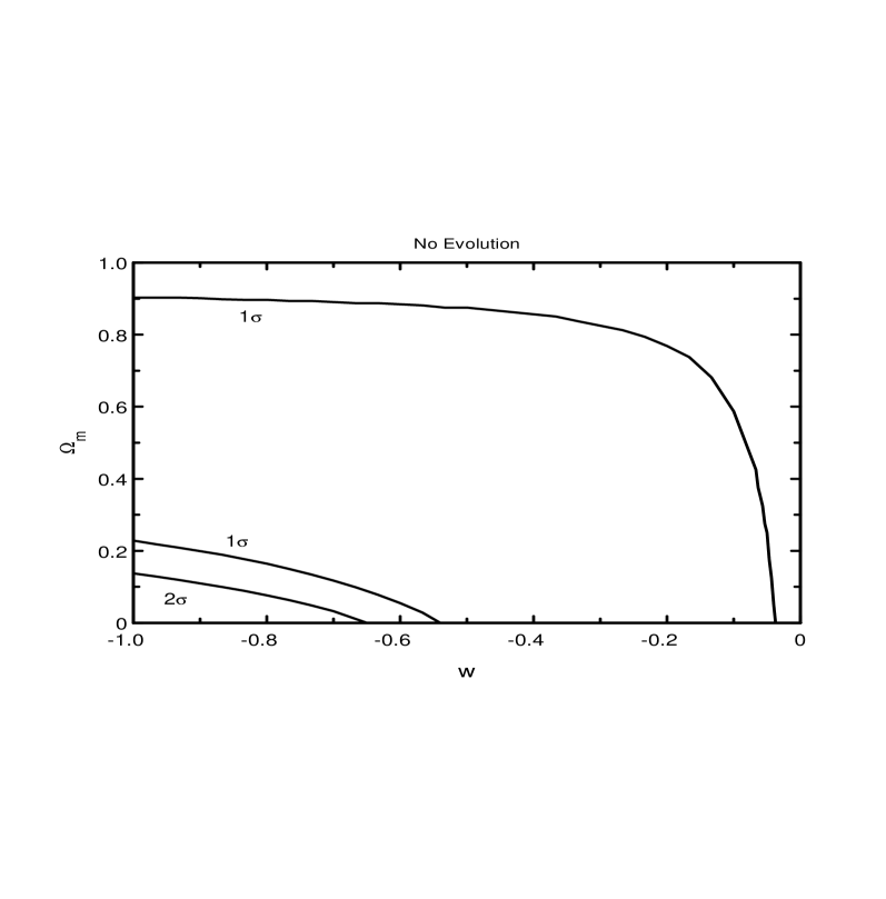
Figure 1: Contours of constant likelihood ($68\%$ and $95.4\%$) for No-Evolution Model for lensing galaxies

$\bullet$ No-Evolution Model : Fig. 1 shows the contours of constant likelihood ($95.4\%$ and $68\%$) in the two parameter space ($w$, $\Omega_{m}$). The best fit (${\mathcal{L}}_{max}$) occurs for $w=-0.33$ and $\Omega_{m}=0.0$. We see that $w\leq-0.04$ and $\Omega_{m}\leq 0.90$ at $1\sigma$ ($68\%$ confidence level). For the case of constant $\Lambda$ i.e. $w=-1.0$, ${\mathcal{L}}_{max}$ occurs for $\Omega_{m}=0.44$ ($\Omega_{\Lambda}=0.56$) and $0.27\leq\Omega_{m}\leq 0.75$ at $1\sigma$. We get $\Omega_{\Lambda}\leq 0.83$ at $2\sigma$ for $w=-1$. Waga & Miceli [64] have done a similar study with Kochaneck’s values [34] for Schechter and lens parameters. For a one parameter fit they get $\Omega_{\Lambda}\leq 0.55$ at $2\sigma$.

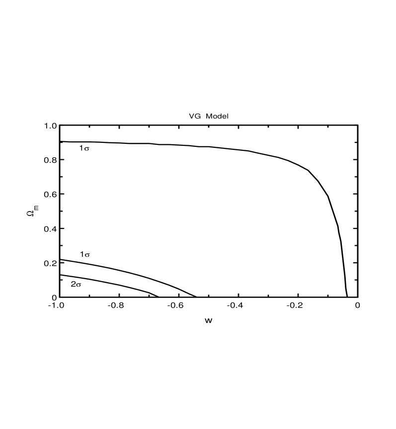
Figure 2: Contours of constant likelihood ($68\%$ and $95.4\%$) for Volmerange & Guiderdoni Model of galaxy evolution.

$\bullet$ VG Model : Fig. 2 summarises the results for the VG Model. The maximum of likelihood occurs for $w=-0.33$ and $\Omega_{m}=0.0$ with $w\leq-0.04$ and $\Omega_{m}\leq 0.91$ at $1\sigma$. For the constant $\Lambda$ case, ${\mathcal{L}}_{max}$ occurs for $\Omega_{m}=0.44$. Also $0.26\leq\Omega_{m}\leq 0.74$ at $1\sigma$ and $\Omega_{m}\geq 0.17$ at $2\sigma$.

$\bullet$ Fast Merging Model : Fig. 3 shows the contours of constant likelihood ($68\%$ and $95.4\%$) for the Fast Merging Model of galaxy evolution. The best fit occurs for $w=-0.26$ and $\Omega_{m}=0.0$. For this model of galaxy evolution the constraints are very weak. For a one parameter fit i.e. for the case of constant $\Lambda$, ${\mathcal{L}}_{max}$ occurs for $\Omega_{m}=0.52$ and $0.29\leq\Omega_{m}\leq 0.92$ at $1\sigma$ and $\Omega_{m}\geq 0.16$ at $2\sigma$.

Table 1 summarises the results for the three models.

Torres and Waga [5], Waga and Miceli [64] have done a similar study for decaying $\Lambda$ cosmologies ($\rho_{\Lambda}\propto a^{-m}$) without taking evolution of galaxies into account. They point out the fact that the constraints obtained from gravitational lens statistics are very weak in these decaying $\Lambda$ cosmologies. The reason for this is that the distance to an object is smaller (for fixed $z$ and $\Omega_{m}$ ) in decaying $\Lambda$ models as compared to the distance of the same object in constant $\Lambda$ models for the same value of $z$ and $\Omega_{m}$. Hence the probability of lensing of that object is reduced in decaying $\Lambda$ model cosmologies. Therefore the constraints on $m$ from the statistics of lensing become weaker.

In this paper our main aim is to check how the constraints on $w$ changes when we include galaxy evolution into the lensing statistics ( in dynamical $\Lambda$ models : X - matter cosmology i.e. $\rho_{x}\propto a^{-3(1+w)}$) . It is a well known fact that the lensing probability depends upon the source redshift, luminosity of the quasar, lens model, the cosmological model and more importantly on the number density of galaxies (lenses). The evolution of galaxies changes the number density of galaxies and hence the probability of lensing changes.

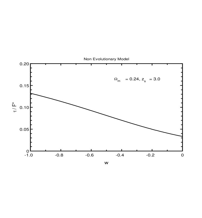
Figure 4: Probability of lensing as a function of $w$

Fig. 4 illustrates how the optical depth (lensing probability) decreases with increasing $w$. This is because as $w$ increases, the distance to an object at redshift $z$ decreases which in turn decreases the probability of lensing. The inclusion of galaxy evolution further decreases the lensing probability in dynamical $\Lambda$ models ( X - matter cosmology ). As a result the constraints on the cosmological parameters ($w$, $\Omega_{m}$) become weaker. In the case of a two parameter fit, we observe that higher values of $w$ permit only low values of $\Omega_{m}$.

The probability for a quasar to get lensed decreases marginally when we go from no-evolution model to VG model for galaxy evolution and hence the constraints on $w$ and $\Omega_{m}$ obtained in the case of the VG model are similar to those obtained in the no-evolution model. On the other hand, the probability for a quasar to get lensed decreases considerably when we work with Fast Merging model for galaxy evolution This gets reflected as weaker constraints in the Fast Merging model. Jain et al. [29] constrained $\Omega_{\Lambda}$ (constant $\Lambda$) for flat cosmologies taking into account galaxy evolution. They worked with the BFSP quasar sample. They constrained it using the information of the number of lensed quasars and concluded that evolution permits a larger value of $\Omega_{\Lambda}$. They also found that in their formalism $\gamma=4$ masks the difference which the evolution of galaxies makes. We would like to point out that the present formalism allows us to study the difference which comes in when the evolution of galaxies is taken into account even with $\gamma=4$.

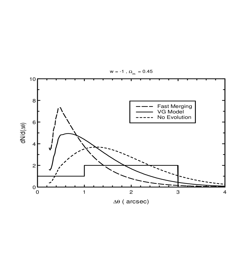
Figure 5: Predicted image-separation distribution $dN/d(\Delta\theta)$ compared with the observed image-separation in the optical quasar sample(histogram).

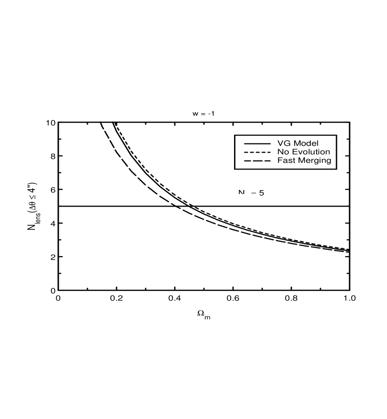
Figure 6: Pridicted number of lensed quasars with $\Delta\theta\leq 4^{\prime\prime}$ in the adopted optical quasars sample.

It is interesting to note that the image separation distribution is different for the three models (Fig. 5). This image separation is sensitive to lens, Schechter and cosmological parameters [30]. Fig. 6 gives the predicted number of lenses $N_{lens}$ in the adopted quasar sample for different $\Omega_{m}$ values ($w=-1$ case) in the three models. The results are similar to those obtained by Jain et al.. i.e. [29]the evolutionary models permit larger values of $\Omega_{\Lambda}$. The constraint that in the given optical sample $N_{L}=5$ gives us different values of $\Omega_{\Lambda}$ in different models.

1. No evolution: $\Omega_{\Lambda}\sim 0.54$

2. VG model: $\Omega_{\Lambda}\sim 0.56$

3. Fast merging model: $\Omega_{\Lambda}\sim 0.60$

In the calculation of number of lensed quasars, $N_{L}$ in the given sample (Fig.6), no information of image morphology is taken into account as explained in Sec. 4.1. Likelihood analysis, on the other hand, takes into account the observed image separations. There is not much difference in the predicted values of $\Omega_{\Lambda}$ by these two methods in the case of no evolution and the VG model for $(w=-1)$ as can be seen by comparing the above mentioned values to those in Table 1. However, for the constant $\Lambda$ case, likelihood analysis shows that the Fast Merging model permits higher values of $\Omega_{m}$ . Calculating the predicted number of lensed quasars and constraining the parameters using the observational fact that in the adopted quasar sample there are five lenses does not make use of the information about the image separations observed for the lensed quasars. The results of likelihood analysis, however, crucially depend on the information about image separation. We feel that it is important to incorporate the image separations information while predicting (constraining) the cosmological parameters.

The constraints obtained from lensing statistics are sensitive to both lens and Schechter parameters [12, 31]. For the quasar luminosity function used in this paper, it is observed that for the case of one parameter fit ( $w=-1$) K96 parameters (Table 2) give $N_{L}=5$ ( for this optical sample of 867 quasars) only when $\Omega_{m}$ is nearly equal to one. For all other values of $\Omega_{m}$, K96 parameters give $N_{L}$ greater than the observed number of lensed quasars (there are five observed lensed quasars) in this optical quasar sample. The LPEM parameters, on the other hand, give numbers around this observed number of lensed quasars over a wide range of parameter ($\Omega_{m}$) values. We have therefore restricted ourselves to the use of LPEM lens and Schechter parameters to study how the galaxy evolution models change the constraints on the cosmological paramters. We observe that the probability for a quasar to get lensed increases with decrease in $\Omega_{m}$ or/and $w$. Therefore for small values of $\Omega_{m}$ and $w$ we cannot use the approximation $\ln(1-p_{i}^{{}^{\prime}})\sim-p_{i}^{{}^{\prime}}$ (in eq. 42) which holds when $p_{i}^{{}^{\prime}}\ll 1$. Infact, for consistency, we have not worked with this approximation for the entire range of the cosmological parameters.

It is interesting to note that with K96 parameters, the lensing probability of a few bright quasars at high redshift becomes greater than one for $\Omega_{m}\sim 0.0$ and $w\sim-1$. For instance, one quasar in the sample with z = 3.02 and $m_{B}=16.1$ gives a probablity($p_{i}^{{}^{\prime}}$) of 1.42 for $\Omega_{m}=0.0$ and $w=-1$. This is not an artifact of our numerical programming and can be checked easily by using either eq. (37) of this paper or eq. (4.15) of K93 [33]. It may be because of the specific values of parameters that we have taken. Specifically, the value of $F^{*}$ for K96 parameters ($F^{*}=0.026$) is quite large as compared to that for the LPEM parameters ($F^{*}=0.010$). Clearly this larger value of $F^{*}$ pushes up the probabilities significantly. In fact, even for those sample points where the probability is less than one, there are instances where the probability is large enough ( near $\Omega_{m}\sim 0.0$ ) so that the approximation $\ln(1-p_{i}^{{}^{\prime}})\sim-p_{i}^{{}^{\prime}}$ is invalid.

It could also be that the formalism itself is inconsistent, though there is no obvious inconsistency when parameters other than K96 are used. If the problem is that of the formalism not being consistent, then one would need to investigate exactly what is it in the formalism which leads to these seemingly absurd probability values.

The strength of the constraints obtained also depends strongly on the lensing data. Extended surveys are required to establish $n(\Delta\theta)$ as a powerful tool for constraining the parameters. The upcoming Sloan Digital Sky Survey which is going down to $1-\sigma$ magnitude limit of $\sim 23$ will definitely increase our understanding of lensing phenomena and cosmological parameters. A large number of new gravitational lens systems $(\sim 18)$ have been discovered by the Cosmic Lens All-Sky Survey (CLASS)[59, 52] . CLASS is the largest survey with more than 10,000 radio sources down to a 5 GHz flux density of 30 mJy. But the major disadvantage of a radio lens survey is that there is little information on the redshift-dependent number-magnitude relation. This leads to serious systematic uncertainties in the derived cosmological constraints.

In this work we have included the effects of galaxy evolution to constrain the cosmological parameters ($w$, $\Omega_{m}$) obtained from lensing statistics. We find that while the constraints obtained in the case of VG model are similar to those obtained for the no evolution case, they are much weaker in the case of the Fast Merging model. We have only considered those galaxy evolutionary models which are based on the assumption that the total comoving mass is conserved during mergers. There is a possibility that the total comoving mass isn’t conserved when mergers take place. Work is under progress to see how lensing statistics and cosmological parameters are affected when total comoving mass density of lenses is not conserved.

Model	Fit	Best Fit	$68\%$ CL	$95.4\%$ CL
		$w$, $\Omega_{m}$
No-Evolution	A	-0.33, 0.0	$w\leq-0.04$
			$\Omega_{m}\leq 0.90$
	B	0.44	$0.27\leq\Omega_{m}\leq 0.75$	$0.17\leq\Omega_{m}$
VG	A	-0.33, 0.0	$w\leq-0.04$
			$\Omega_{m}\leq 0.91$
	B	0.44	$0.26\leq\Omega_{m}\leq 0.74$	$0.17\leq\Omega_{m}$
Fast Merging	A	-0.26, 0.0
	B	0.52	$0.29\leq\Omega_{m}\leq 0.92$	$0.16\leq\Omega_{m}$

Table 1: Here A refers to the two parameter fit and B refers to one parameter fit i.e. when $w=-1$.

Survey	$\alpha$	$\phi_{\ast}(h^{3}\,Mpc^{-3})$	$v_{\ast}(km/s)$	$F^{*}$
LPEM	+0.2	$3.2\times 10^{-3}$	205.3	0.010
K96	-1.0	$6.1\times 10^{-3}$	225.0	0.026

Table 2: Lens and Schecter Paramters for E/SO galaxies

Figure 3: Contours of constant likelihood ($68\%$ and $95.4\%$) for Fast Merging Model of galaxy evolution.

References

- [1] Bahcall, J. N., et al. 1992, ApJ, 387, 56
- [2] Baugh, C. M.,Cole, S., & Frenk, C. S. 1996, MNRAS, 282, L27
- [3] Baugh, C. M., Cole, S., & Frenk, C. S. 1996, MNRAS, 283, 1361
- [4] Baugh, C. M., et al. 1998, ApJ, 498, 504
- [5] Bloomfield Torres, L. F., & Waga, I. 1996, MNRAS, 279, 712
- [6] Broadhurst, T., Ellis, R., & Glazebrook, K. 1992, Nature, 355, 55 [BEG]
- [7] Burkey, J. M., et al. 1994, ApJ, 429, L13
- [8] Caldwell, R. R., Dave, R., & Steinhardt, P. J. 1998 Phy. Rev. Lett., 80, 1582
- [9] Carlberg, R. G., et al. 1994, ApJ, 435, 540
- [10] Chiba, T., Sugiyama, N., & Nakamura, T. 1997, MNRAS, 289, L5
- [11] Chiba, T., Sugiyama, N., & Nakamura, T. 1998, MNRAS, 301, 72
- [12] Chiba, M. & Yoshii, Y. 1999, ApJ, 510, 42
- [13] Cole, S., et al. 1994, MNRAS, 271, 781
- [14] Crampton, D., McClure, R. D., & Fletcher, J. M. 1992, ApJ, 392, 23
- [15] de Bernardis, P., et al. 2000, Nature, 404, 955
- [16] Driver, S. P., et al. 1995, ApJ, 449, L23
- [17] Efstathiou, G. 1999, preprint astro-ph/9904356
- [18] Eggen, O. J., Lynden-Bell, D., & Sandage, A. R. 1962, ApJ, 136, 748
- [19] Ellis, R. S., et al. 1996, MNRAS, 280, 235
- [20] Ellis, R. S. 1997, ARA&A, 35, 389
- [21] Faber, S. M., et al. 1976, ApJ, 204, 668
- [22] Fukugita, M., & Turner, E. L. 1991, MNRAS, 253, 99
- [23] Fukugita, M., Futamase, T., Kasai, M., & Turner, E. L. 1992, ApJ, 393, 3
- [24] Glazebrook, K., et al. 1995, MNRAS, 273, 157
- [25] Guiderdoni, B., & Rocca-Volmerange, B. 1991, A&A, 252, 435
- [26] Gunn, J. E., & Gott, J. R. 1997, ApJ, 176, 1
- [27] Hartwich, F. D. A., & Schade, D. 1990, ARA&A, 28, 437
- [28] Huterer, D., & Turner, M. S. 1999, Phy. Rev. D, 60, 081301
- [29] Jain, D., Panchapakesan, N., Mahajan, S., & Bhatia, V. B. 1998, Int.J. Mod. Phys., A13, 4227
- [30] Jain, D., Panchapakesan, N., Mahajan, S., & Bhatia, V. B. 2000, Mod. Phys. Lett A, 15, 41
- [31] Jain, D. et al., 2001, preprint astro-ph/0105551
- [32] Jaunsen, A. O., Jablonski, M., Petterson, B. R., & Stabell, R. 1995, A&A, 300, 323
- [33] Kochanek, C. S. 1993, ApJ, 419, 12 [K93]
- [34] Kochanek, C. S. 1996, ApJ, 466, 638 [K96]
- [35] Kochanek, C. S., Falco, E. E., & Schild, R. 1995, ApJ, 452, 109
- [36] Lampton, M., Margon, B., & Bowyer, S. 1976, ApJ, 208, 177
- [37] Lima, J. A. S., & Alcaniz, J. S. 2000, MNRAS, 317, 893
- [38] Lilly, S. J., et al. 1995, ApJ, 455, 108 (1995)
- [39] Loveday, J.,Peterson, B. A., Efstathiou, G.,& Maddox, S. J. 1992, ApJ, 390, 338 (LPEM)
- [40] Mao, S., & Kochanek, C. S. 1994, MNRAS, 268, 569
- [41] Maoz, D., et al. 1993, ApJ, 409, 28 (Snapshot)
- [42] Ostriker, P.J., & Steinhardt, P. J. 1995, Nature, 377, 600
- [43] Partridge, R. B., & Peebles, P. J. E. 1967, ApJ, 147, 868
- [44] Peebles, P. J. E. 1984, ApJ, 284, 439
- [45] Perlmutter, S., et al. 1999, ApJ, 517, 565
- [46] Perlmutter, S., et al. 1999 Phy. Rev. Lett., 83, 670 (1999)
- [47] Press, W. H., & Schechter, P. 1974, ApJ, 187, 487
- [48] Ratra, B., & Peebles, P. J. E. 1988 Phy. Rev. D, 37, 3406
- [49] Riess, A. G., et al. 1998, AJ., 116, 1009
- [50] Rix, H. W., Maoz, D., Turner, E., & Fukugita, M. 1994, ApJ, 435, 49
- [51] Rocca-Volmerange, B., & Guiderdoni, B. 1990, MNRAS, 247, 166
- [52] Rusin, D & Tegmark, M. Preprint No. astro - ph/0008329 (2000)
- [53] Sahni, V., & Starobinsky, A. 2000, Int. J. Mod. Phys., D9, 373
- [54] Schechter, P. 1976, ApJ, 203, 297
- [55] Schwezier, F. 1996, AJ, 111, 109
- [56] Silveira, V., & Waga, I. 1994, Phys. Rev. D, 50, 4890
- [57] Silveira, V., & Waga, I. 1997, Phys. Rev. D, 56, 4625
- [58] Surdej, J., et al. 1993, AJ, 105, 2064
- [59] Takahashi, R. & Chiba, T. Preprint No. astro - ph/0106176 (2001)
- [60] Toomre, A. 1997, in The Evolution of Galaxies and Stellar Populations eds: B. M. Tinsley & R. B. Larson ( Yale Univ. Observatory), p-401
- [61] Turner, E. L.,Ostriker, J. P., & Gott III, J. R. 1984, ApJ, 284, 1
- [62] Turner, E. L. 1990, ApJ, 365, L43
- [63] Turner, M. S., & White, M. 1997, Phy. Rev. D, 56, 4439
- [64] Waga, I., & Miceli, A. P. M. R. 1999, Phy. Rev. D, 59, 103507
- [65] Wang, et al. 2000, ApJ, 530, 17
- [66] Yee, H. K. C., Filippenko, A. V., & Tang, D. 1993, AJ, 105, 7
- [67] Yee, H. K. C., & Ellingson, E. 1995, ApJ, 445, 37
- [68] Zepf, S. E., & Koo, D. C. 1998, ApJ, 337, 34
- [69] Zepf, S. E. 1997, Nature, 390, 377
- [70] Zhu, Z. H. 2000, Int. J. Mod. Phys., D9, 591