Macrolensing signatures of large-scale violations of the weak energy condition

Abstract

We present a set of simulations of the macrolensing effects produced by large-scale cosmological violations of the energy conditions. These simulations show how the appearance of a background field of galaxies is affected when lensed by a region with an energy density equivalent to a negative mass ranging from $10^{12}$ to $10^{17}$ $|M_{\odot}|$. We compare with the macrolensing results of equal amounts of positive mass, and show that, contrary to the usual case where tangential arc-like structures are expected, there appear radial arcs—runaway filaments—and a central void. These results make the cosmological macrolensing produced by space-time domains where the weak energy conditions is violated, observationally distinguishable from standard regions. Whether large domains with negative energy density indeed exist in the universe can now be decided by future observations of deep fields.

Introduction

The energy conditions (EC) of classical General Relativity (see Appendix) are conjectures widely used to prove theorems concerning singularities and black hole thermodynamics. The area increase theorem for black holes, the topological censorship theorem, and the singularity theorem of stellar collapse, are among the most important ones [1]. However, the set of EC constitute only plausible statements, all of them lacking a rigorous proof. Moreover, several situations in which the EC are violated are known; perhaps the most quoted being the Casimir effect. For other physical situations see Ref. [2] and references therein. Typically, observed violations are produced by small quantum systems, resulting of the order of $\hbar$. It is currently far from clear whether there could be macroscopic quantities of such an exotic, EC-violating, matter.

The violations of the EC, in particular the weak one, would admit the existence of negative amounts of mass. As Bondi remarked in Ref. [4], it is an empirical fact that inertial and gravitational masses are both positive quantities. In fact, the possible existence of negative gravitational masses is being investigated at least since the end of the nineteen century [3]. The empirical absence of negative masses in the Earth neighborhood could be explained as the result of the plausible assumption that, repelled by the positive masses prevalent in our region of space, the negative ones have been driven away to extragalactic distances. Recently, primordially formed negative gravitational masses have been proposed as an explanation of the voids observed in the extragalactic space [5]. Mann [6] have found, in addition, that dense regions of negative mass can undergo gravitational collapse, probably ending up in exotic black holes.

Of all the systems which would require violations of the EC in order to exist, wormholes are the most intriguing [7]. The most salient feature of these objects is that an embedding of one of their space-like sections in Euclidean space displays two asymptotically flat regions joined by a throat. Observational properties of stellar and sub-stellar size wormholes have been recently discussed in the literature; the propagation of perturbations and particles [8], the possible violation of the equivalence principle [9], the gravitational lensing of light [10], and the possibility of relating them with gamma-ray bursts [11] are some examples. In all these cases, however, wormholes were considered as compact objects formed by about 1 negative solar mass.

Very recently, the consequences of the validity of the EC were confronted with possible values of the Hubble parameter and the gravitational redshifts of the oldest stars [12]. It was deduced that the strong energy condition (considering the density of the universe as a whole) can be violated rather late in the history of the universe, sometime between the formation of the oldest stars and the present epoch. This would imply the existence of a massive scalar field or a positive cosmological constant, something what recent experiments seem to favor. But even if the global energy density of the universe is WEC-respecting, we can wonder whether there exist space-time domains where large-scale violations of the EC occur, allowing the formation of physical systems with an energy density equivalent to a total negative mass of the size of a galaxy or even a cluster of galaxies.

If the answer to this question is yes, it is clear that we should be able to see some gravitational effects on the light that traverse such regions. In particular, lensing of distant background sources should exhibit distinctive features. In what follows, we present the results of a set of simulations showing the macrolensing effects we could observe if such a large amount of negative energy density exist in our universe.

Lens equation and description of the algorithm

We begin the discussion of gravitational lensing by defining two convenient planes, i.e. the source and lens plane. These planes, described by Cartesian coordinate systems ($\beta_{1},\beta_{2}$) and ($\theta_{1},\theta_{2}$), pass through the source and the deflecting mass, respectively, and are perpendicular to the optical axis (the straight line joining the source plane, through the deflecting mass, and the observer). We write the gravitational lens equation, which governs the mapping from the lens to the source plane, in dimensionless form

$$\mbox{\boldmath$\beta$}=\mbox{\boldmath$\theta$}\left[1+\frac{\theta^{2}_{\rm E}}{\theta^{2}}\right]\,\,,$$ (1)

where $\beta$($\theta$) refers to the position of the source (image) on the sky, as described in the Fig. 1. We have defined the quantity $\theta_{\rm E}$ in analogy with lensing by positive matter as

$$\theta^{2}_{\rm E}=\frac{4G|M|}{c^{2}}\frac{D_{\rm ls}}{D_{\rm s}D_{\rm l}}\,\,,$$ (2)

where $D_{\rm l}$, $D_{\rm s}$, and $D_{\rm ls}$ are the angular diameter distances from the observer to the lens, from the observer to the source, and from the lens to the source, respectively. We forward the reader looking for a complete theoretical treatment of lensing by negative masses to Ref. [13]. It should be borne in mind that although $\theta_{\rm E}$ is the only natural angular scale in Eq. (1), it does not have the same physical meaning as in the case of the positive lensing, since negative matter cannot produce an Einstein ring.

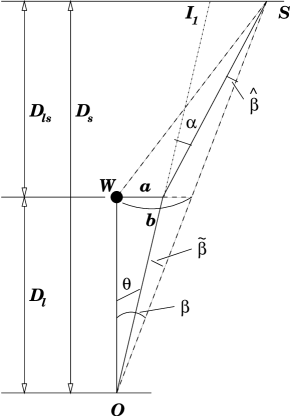
Figure 1: Lensing geometry for a negative mass. $O$ is the observer, $S$ is the source, $W$ is the position of the negative mass and $I_{1}$ is one the images. $\beta$ is the angle between the source and the image, $\alpha$ is the deflection angle. $b$ is the impact parameter, and all other quantities are auxiliary to obtain the lens equation. $D_{\rm l}$, $D_{\rm s}$ and $D_{\rm ls}$ are angular diameter distances.

For the simulations that follow, we have used a background cosmology described by a Friedmann-Robertson-Walker flat universe with $\Omega_{\rm m}=1$ and a zero cosmological constant. In all numerical computations we have used a Hubble parameter $h$ equal to 1 ($H_{0}=100\,h$ km sec^-1 Mpc^-1). The relationship $D_{\rm eff}=D_{\rm l}D_{\rm ls}D_{\rm s}^{-1}$, entering the Eq. 2, is a measure of the lensing efficiency of a given mass distribution. $D_{\rm eff}$ peaks, quite independently of the cosmological model assumed, at a lens redshift of $\sim 0.2-0.4$ for sources at a typical redshift $z_{\rm s}\sim 1-1.3$ [17]. To be more realistic, we shall place the lens at a redshift of $z_{l}=0.3$ and generate a random sample of galaxies in the redshift range $0.3<z_{\rm source}<2.0$. The redshift distribution conserves their comoving number density. This number density and the projected sizes for these background sources were taken to be close to the Tyson population of faint blue galaxies [16]. The luminous area of each galaxy was taken to be a circular disk of radius $R$ with a uniform brightness profile and orientations of disk galaxies were randomly placed in space. NOTE: the next lines you can remove if you want or retain. This was done by defining in the code the ellipticity $e$ ($e=(1-r)/(1+r)$, $r$ is the ratio of the minor axis to the major axis) and the position angle $\varphi$, and randomly chosing the values of $e$ from the range $0<e<0.7$ and the values of $\varphi$ from the range $0<\varphi<2\pi$.

The lens equation (1) describes a mapping ${\bf\theta}\mapsto{\bf\beta}$, from the lens to the source plane. For convenience, we redefine the lens plane as ${\bf x}$ and the source plane as ${\bf y}$. Then, Eq. (1) can be written as

$${\bf y}={\bf x}\left(1+\frac{\theta^{2}_{\rm E}}{x^{2}}\right),$$ (3)

where $x=|{\bf x}|=\sqrt{x_{1}^{2}+x_{2}^{2}}$.

We now consider a source, whose shape—either circular or elliptical—can be described by a function $\chi({\bf y})$. Curves of constant $\chi$ are the contours of the source. One can as well consider $\chi$ as a function of ${\bf x}$, $\chi({\bf y}({\bf x}))$, where ${\bf y}({\bf x})$ is found using the lens equation. Thus, all points ${\bf x}$ of constant $\chi$ are mapped onto points ${\bf y}$, which have a distance $\sqrt{\chi}$ from the centre of the source. If the latter contour can be considered an isophote of a source, one has thus found the corresponding isophotes of the images. See Ref. [15] for further details.

Simulations results

In the first set of figures (Figs. 2-6), we show the results of our simulations. Some special precautions must be taken for the largest masses. The problem is that for a very massive lens the Einstein ring becomes very large. Since for the negative mass lensing all sources inside the double Einstein radius are shadowed (i.e. we can see the images of only those sources which are outside the double Einstein radius), if we were to use for lensing only the sources shown on the window, a fold-four symmetry pattern would appear (Fig. 7). Only the sources at the corners of the current window (and outside the double Einstein radius) are lensed. In order to solve this problem we have to consider also the sources from outside the current window; then the lensing picture is restored and the scale of the simulation is consistently increased. For this reason we increase the number of background galaxies in Figs. 4–6. We show this in detail in Figs. 7 and 8.

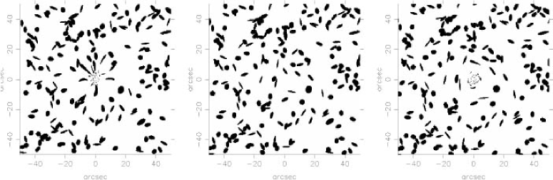
Figure 2: Left: Appearance of a background field of sources in a range of redshifts (see text) (200 galaxies, intrinsic radius 7 Kpc), when lensed by a negative mass of $|M|_{\rm lens}=1\times 10^{13}\,M_{\odot}$. Center: Unlensed background field. Right: Appearance of the same background field of galaxies when it is lensed by an equal amount of positive mass; redhsifts are the same as for the negative mass case.

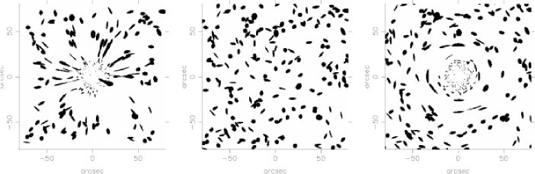
Figure 3: Left: Appearance of a background field of sources (200 galaxies, intrinsic radius 10 Kpc), when it is lensed by a negative mass of $|M|_{\rm lens}=1\times 10^{14}\,M_{\odot}$. Center: As in Figure 2. Right: As in Figure 2.

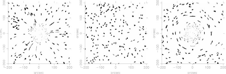
Figure 4: Left: Appearance of a background field of sources (300 galaxies, intrinsic radius 15 Kpc), when it is lensed by a negative mass of $|M|_{\rm lens}=1\times 10^{15}\,M_{\odot}$. The simulation was made taking into account sources located within 1.2 of the size of the shown window. Center: As in Figure 2. Right: As in Figure 2.

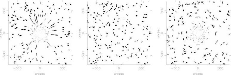
Figure 5: Left: Appearance of a background field of sources (300 galaxies, intrinsic radius 50 Kpc), when it is lensed by a negative mass of $|M|_{\rm lens}=1\times 10^{16}\,M_{\odot}$. The simulation was made taking into account sources located within 1.2 of the size of the shown window. Center: As in Figure 2. Right: As in Figure 2.

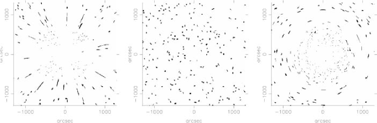
Figure 6: Left: Appearance of a background field of sources (500 galaxies), intrinsic radius 60 Kpc, when it is lensed by a negative mass of $|M|_{\rm lens}=1\times 10^{17}\,M_{\odot}$. The simulation was actually made taking into account sources located within 1.5 of the size of the shown window. Center: As in Figure 2. Right: As in Figure 2.

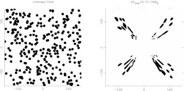
Figure 7: The need for the increase of the background number of sources is shown by the appearance of a four-fold symmetric pattern, which occurs because only the galaxies at the corners of the left window are being affected by lensing effects. Axis are marked in arcseconds. See next figure.

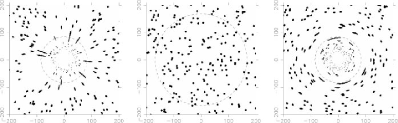
Figure 8: Left: Appearance of a background field of circular sources (300 galaxies), each of them of 15 Kpc radius, when it is lensed by a negative mass of $|M|_{\rm lens}=1\times 10^{15}\,M_{\odot}$ with an Einstein angular radius equal to $\theta_{\rm E}=84$ arcsec. The dashed circle is the Einstein ring, the radial arcs are centered on it while the images inside it are demagnified. Here $z_{\rm lens}=0.4$, $z_{\rm source}=1.4$. The simulation was made taking into account sources located within 1.2 of the size of the shown window. Center: Background field in the absence of the lens, dashed circle is the double Einstein radius, all sources inside this radius are shadowed. Right: Macrolensing effects produced by a positive mass lens of $10^{15}\,M_{\odot}$, a dashed circle is the Einstein radius shown here for comparison, sources inside it are strongly lensed.

As a general feature of our simulations we can remark that, opposite to the standard positive mass case, where ring-like structures appear, the negative mass lensing produce finger-like, apparently “runaway” structures, which seem to escape from a central void. This is in agreement with the appearance of a central umbra in the case of a point-like negative mass lensing, as studied by Cramer et al. [10]. In the case of macrolensing, the umbra (central void) is maintained on a larger scale which, depending on the negative mass of the lens, can reach hundreds of acrsec in linear size. This umbra is always larger than the corresponding one generated in positive macrolensing (see Figures 2-6) and totally different in nature [10]. Then, the existence of a macroscopic amount of negative mass lens can— at least qualitatively—mimic the appearance of galaxy voids.

In order to explore the influence of the adopted redshift values, we turn now to the case where $z_{\rm sources}=0.08$ and $z_{\rm lens}=0.05$. The Bootes void is the closest void to us, and lies between the supercluster Corona Borealis ($z\approx 0.08$) and Hercules ($z\approx 0.03$) [18]. This serves as motivation for the selection of these redshift values. As an example of the results for different lens masses, we show in Figs. 9 and 10 the cases with $|M|_{\rm lens}=1\times 10^{14}\,M_{\odot}$ and $|M|_{\rm lens}=1\times 10^{16}\,M_{\odot}$.

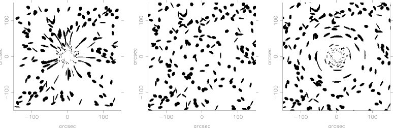
Figure 9: Left: Appearance of a background field of sources (200 galaxies), each of them 5 Kpc radius, when it is lensed by a negative mass of $|M|_{\rm lens}=1\times 10^{14}\,M_{\odot}$ with an Einstein angular radius equal to $\theta_{\rm E}=47$ arcsec. Center: Unlensed background field. Right: Appearance of the same background field of galaxies when lensed by an equal amount of positive mass, located at the same redshift (see text).

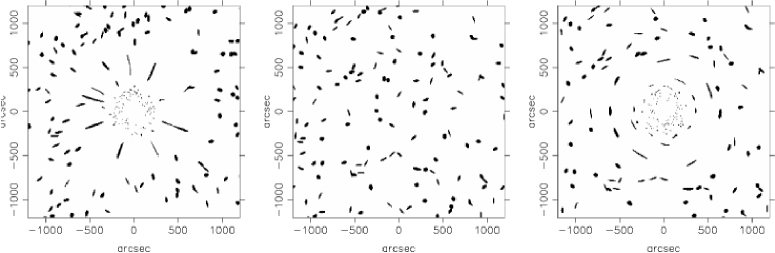
Figure 10: Left: Appearance of a background field of sources (300 galaxies), each of them of 25 Kpc radius, when it is lensed by a negative mass of $|M|_{\rm lens}=1\times 10^{16}\,M_{\odot}$ with an Einstein angular radius equal to $\theta_{\rm E}=467$ arcsec. Center: As in Figure 9. Right: As in Figure 9.

It is interesting to note that although the background population of galaxies is very dense, and for the standard model of cosmology to be valid, one would expect a lot of lensing. However, there is still a surprising dearth of candidates for (positive mass) lensed sources [19]. Some of the richest clusters do not display arcs in the deepest images. CL0016+16 ($z=0.56$), for instance, is one of the richest and strongest X-ray emitter clusters. It is rather extended on the sky, so the light from many background sources should cross this cluster. Neither arcs nor arclets have been found, though weak lensing has been reported. This may be pointing towards a cautionary note: if the kind of finger-like structures displayed in our figures is not directly seen in its full pattern, that does not necessarily mean that they are absent. Even the presence of one radial arc (without tangential counter arc and/or tangential arcs) may be significant.

Concluding remarks

The null EC (NEC) is the weakest of the EC. Usually, it was considered that all reasonable forms of matter should at least satisfy the NEC. However, even the NEC and its averaged version (ANEC) are violated by quantum effects and semi-classical quantum gravity (quantized matter fields in a classical gravitational background). Moreover, it has recently been shown that there are also large classical violations of the energy conditions [20]. This Letter shows that—disregarding the fundamental mechanism by which the EC are violated, e.g. fundamental scalar fields, modified gravitational theories, etc.—if large localized violations of NEC exist in our universe, we can be able to detect them through cosmological macrolensing. Contrary to the usual case, where ring structures are expected, finger-like, “runaway” filaments and a central void appear. Figures 2–6 and 9–10 compare with the case of macrolensing effects on background fields produced by equal amounts of positive mass located at the same redshift. Differences are notorious. These results make the cosmological macrolensing produced by matter violating the weak energy condition observationally distinguishable from the standard situation. Whether large-scale violations of the EC resulting in space-time regions with average negative energy density indeed exist in the universe can now be decided through observations.

Appendix: Energy conditions

To specify what we are referring to when talking about the energy conditions, we provide their point-wise form. They are the null (NEC), the weak (WEC), the strong (SEC), and the dominant (DEC) energy conditions. Using a Friedmann-Robertson-Walker space-time and the Einstein field equations, they read:

NEC $$\iff \quad(\rho+p\geq 0),$$

WEC $$\iff \quad(\rho\geq 0)\hbox{ and }(\rho+p\geq 0),$$

SEC $$\iff \quad(\rho+3p\geq 0)\hbox{ and }(\rho+p\geq 0),$$

DEC $$\iff \quad(\rho\geq 0)\hbox{ and }(\rho\pm p\geq 0).$$ (4)

The EC are, then, linear relations between the energy and the pressure of the matter generating the space-time curvature.

References

- [1] M. Visser, Lorentzian Wormholes, (AIP, New York, 1996).
- [2] D. Hochberg, A. Popov, and S. V. Sushkov, Phys. Rev. Lett. 78, 2050 (1997); S. Kim and H. Lee, Phys. Lett. B458, 245 (1999); S. Hayward, Int. J. Mod. Phys. D8, 373 (1999); S. Krasnikov, Phys. Rev. D62, 084028 (2000); L.A. Anchordoqui, S. E. Perez Bergliaffa and D. F. Torres, Phys. Rev. D55, 5226 (1997); C. Barceló and M. Visser, Phys. Lett. B466, 127 (1999); Class. Quant. Grav. 17, 3843 (2000); A. DeBenedictis and A. Das, [gr-qc/0009072].
- [3] M. Jammer, Concepts of mass, (Dover, New York, 1997).
- [4] H. Bondi, Rev. Mod. Phys. 29, 423 (1957).
- [5] T. Piran, Gen. Rel. Grav. 29, 1363 (1997).
- [6] R. Mann, Class. Quant. Grav. 14, 2927 (1997).
- [7] M. S. Morris and K. S. Thorne, Am. J. Phys. 56, 395 (1987); M. Morris, K. Thorne and U. Yurtserver, Phys. Rev. Lett. 61, 1446 (1988).
- [8] S. Kar, D. Sahdev, and B. Bhawal, Phys. Rev. D49, 853 (1994). S. E. Perez Bergliaffa and K. E. Hibberd, Phys. Rev. D62, 044045 (2000); G. Lambiase, S. Capozziello, D. F. Torres, and L. A. Anchordoqui, Submitted 2001.
- [9] L. A. Anchordoqui, S. Capozziello, G. Lambiase and D. F. Torres, Mod. Phys. Lett. A15, 2219 (2000).
- [10] J. Cramer, R. Forward, M. Morris, M. Visser, G. Benford, and G. Landis, Phys. Rev. D51, 3117 (1995).
- [11] D. F. Torres, G. Romero, L. Anchordoqui, Phys. Rev. D58, 123001 (1998); Mod. Phys. Lett. A13, 1575 (1998). L. Anchordoqui, G. E. Romero, D. F. Torres and I. Andruchow, Mod. Phys. Lett. A14, 791 (1999); G. E. Romero, D. F. Torres, I. Andruchow, L. A. Anchordoqui and B. Link, Mon. Not. R. Ast. Soc. 308, 799 (1999).
- [12] M. Visser, Phys. Rev. D56, 7578 (1997); Science 276, 88 (1997).
- [13] M. Safonova, D. F. Torres and G. E. Romero, in preparation (2001).
- [14] W. H. Press, S. A. Teukolsky, W. T. Vetterling & B. P. Flannery Numerical Recipes in FORTRAN, edition (Cambridge University Press, Cambridge, England, 1992).
- [15] P. Schneider, J. Ehlers & E. E. Falco, Gravitational lenses (Springer-Verlag, Berlin, 1992).
- [16] J. A. Tyson, Astron. J 96, 1 (1988).
- [17] M. Bartelmann, A. Huss, J. M. Colberg, A. Jenkins & F. R. Pearce, Large Scale Structure: Tracks and Traces. Proceedings of the 12th Potsdam Cosmology Workshop, held in Potsdam, September 15th to 19th, 1997. Eds. V. Mueller, S. Gottloeber, J.P. Muecket, J. Wambsganss World Scientific 1998, p. 321-324.
- [18] N. A. Bahcall and R. M. Soneira, Astrophys. Lett. 258, L17 (1982).
- [19] A. R. Cooray, J. M. Quashnock, and M. C. Miller, Astrophys. J. 511, L562 (1999).
- [20] E. E. Flanagan and R. M. Wald, Phys. Rev. D54, 6233 (1996); M. Visser and C. Barcelo, [gr-qc/000109].