FLIERs as stagnation knots from post-AGB winds with polar momentum deficiency

Abstract

We present an alternative model for the formation of fast low-ionization emission regions (FLIERs) in planetary nebulae that is able to account for many of their attendant characteristics and circumvent the problems on the collimation/formation mechanisms found in previous studies. In this model, the section of the stellar wind flowing along the symmetry axis carries less mechanical momentum than at higher latitudes, and temporarily develops a concave or inverted shock geometry. The shocked ambient material is thus refracted towards the symmetry axis, instead of away from it, and accumulates in the concave section. The reverse is true for the outflowing stellar wind, which in the reverse shock is refracted away from the axis. It surrounds the stagnation region of the bow-shock and confines the trapped ambient gas. The latter has time to cool and is then compressed into a dense ”stagnation knot” or ”stagnation jet”. In the presence of a variable stellar wind these features may eventually overrun the expanding nebular shell and appear as detached FLIERs. We present representative two and three-dimensional hydrodynamic simulations of the formation and early evolution of stagnation knots and jets and compare their dynamical properties with those of FLIERs in planetary nebulae.

Subject Headings: hydrodynamics - ISM: jets and outflows - ISM: kinematics and dynamics - planetary nebulae: FLIERs and stagnation knots

1 Introduction and model description

FLIERs in planetary nebulae were originally identified with the structures previously known as ansae in elliptical planetary nebulae (Aller, 1941; Balick et al. 1993). Their peculiar characteristics are now recognized in a much wider variety of PNe (e.g. Guerrero, Vázquez & López 1999; Goncalves et al. 2000). Their nature has resisted a consistent explanation to date. Initially, FLIERs were considered as pairs of knots located symmetrically with respect to the PN nucleus and characterised by outflow radial velocities of the order of 30-50 ${\rm\ km\ s}^{-1}$. Ionization gradients decrease outwards from the nebular core and in often ‘head-tail’ morphologies are observed (see Balick et al. 1998).

However, and as pointed out by López (2000), the concept of FLIERs has been used in recent times to encompass nearly any [N II] bright knot in the periphery of PN-shells found to be traveling either with nearly null or very high radial velocity. A single model can hardly account for all the properties observed. Symmetric ejecta, shocks, recombination fronts or simply dynamical instabilities may form in the nebular rim developing dense, low ionization knots and expanding with the rim. These effects have not always been distinguished.

Regarding the observed position and velocities, projection effects have to be taken into account as well. A number of symmetric FLIERs, like the outer pair in NGC 7009, appear to be nearly aligned with the plane of the sky. Although they show only a few ${\rm\ km\ s}^{-1}$ radial velocity, the deprojected speed is estimated by Reay & Atherton (1985) as 160 (D/2) km/s, with D the distance in kpc. In some sources with extended ansae or strings of symmetric knots a linear increase of speed with distance has been found with values rising up to $\approx 630$ ${\rm\ km\ s}^{-1}$(Bryce et al. 1997, Corradi et al. 1999, O’Connor et al. 2000). Obviously, FLIERs are only part of a much richer variety of dynamic phenomena in PNe.

Models have proliferated with varying degrees of success in explaining the observed properties of these structures. For example, ionization fronts (IF) in localized dense knots and collimated flows which produce fast knots ramming through the shell of the PN have been discussed by Balick et al. (1998). Dopita (1997) has discussed FLIERs in terms of shocks immersed in the strongly radiative PN environment.

FLIERs do not usually show a physical connection between themselves and the nebular core. This fact has to be accounted for by any collimation model. In this regard, Frank, Balick & Livio (1996) discussed the case of a cooling wind that avoids fast reexpansion via a collimation mechanism similar to the one described by Cantó et al. (1988). In this model the wind slides along the aspherical outer shock towards the axis forming a dense, narrow jet. Alternatively, Redman & Dyson (1999) have presented a model in which FLIERs represent recombination fronts (RF) in mass-loaded jets.

On a different approach, García-Segura & López (2000) have recently developed 3D magneto- hydrodynamic models which successfully reproduce ansae-type structures by considering a shocked stellar wind carrying a toroidal magnetic field (see Ró$\dot{\rm z}$yczka & Franco, 1996) with mass-loss rates $\leq$ 10^-7 M_⊙ yr^-1. Above this limit, jet structures develop in their model. In the MHD model, and the others mentioned above, the material cooling to form FLIERs comes from the stellar wind or a mixture with material from the ambient (in the case of mass-loading).

In this paper we elaborate on an alternative hydrodynamical model for the formation of axial, high-velocity ansae, introduced by Steffen & López (2000). In this model, FLIERs are formed from external gas swept-up by a fast, low-density wind plowing into the ambient medium of the PN, the latter formed from the slow dense wind of the central star during its AGB phase. It is worth noting that the group of elliptical nebulae with typical FLIERS show very extended halos, such as NGC 3242 (Meaburn, López & Noriega-Crespo, 2000) and NGC 7009 (Moreno-Corral, de la Fuente & Gutierrez, 1998)

1.1 The stagnation knot model

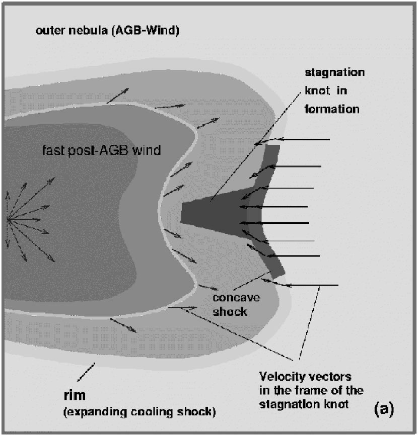
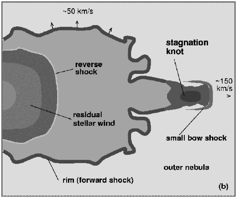
Figure 1: Schematic view of the early evolution of stagnation knot during the phase of a concave bow-shock (Panel a). The arrows near the origin represent the moment flux in the fast wind and are drawn in the rest frame of the central star. The arrows in the bow-shock region are velocities of the shocked fast wind (left) and the shocked external medium (right) in the rest frame of the stagnation knot. They illustrate the divergent flow of the fast wind and the convergence of the slow wind. Panel b illustrates the late stage of evolution during which the stagnation feature has separated from rim of the planetary nebula.

The idea of a ”stagnation knot” was used for the first time to reproduce the large-scale structure of the giant envelope of the PN KjPn8 (Steffen & López, 1998). We have generalized the model in such a way that it is able to produce symmetric high-density knots of jets from an uncollimated stellar wind or even from precessing jets. In our model, we postulate that there is a fast low-density outflow from the central object of a planetary nebula with a deficiency of momentum along the symmetry axis of the nebula (as compared to the momentum flowing along higher latitudes, see Figure 1a). The deficiency of momentum flux along the axis may arise from an interacting binary system, as described by Soker & Rappaport (2000). Alternatively, precessing collimated outflows or jets produce conical outflows (Peter & Eichler, 1995, and Lim, 2001) which also have the required flow geometry.

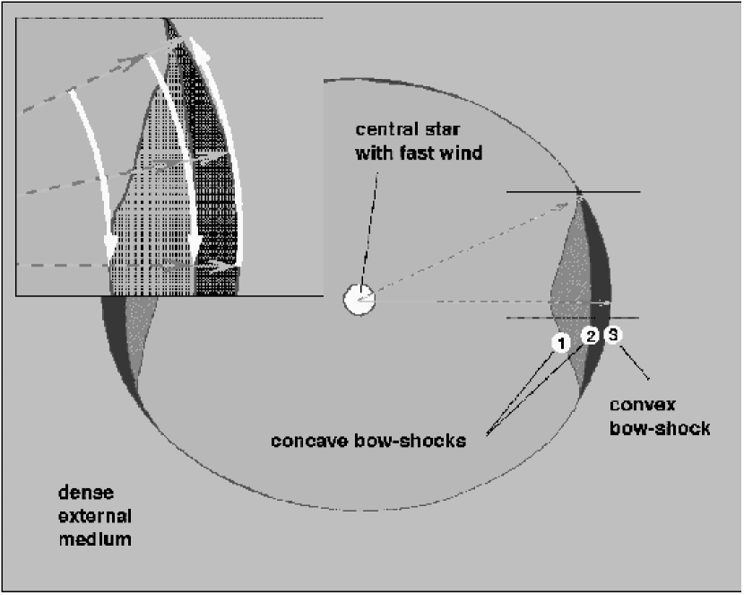
Figure 2: Schematic view of an elliptical shock wave of the fast stellar wind moving into the external medium with different bow-shock structures near the symmetry axis. Three qualitatively different cases are shown. Case 1 is a clearly concave bow-shock. Case 2 is geometrically convex or almost planar, but with respect to the spherical wind it acts as a concave shock (see inset were the position of the shock wave is shown with respect to the flow lines of the stellar wind). Case 3 is the normal convex bow-shock. The white arrows in the inset indicate the tangential lines to the stellar wind and the directions of the pressure gradient produced by the shocked fast stellar wind.

The reduced momentum flux along the axis causes the bow-shock to advance more slowly near the axis and hence the shock becomes concave instead of convex (as seen from outside; see Figure 2). The ambient medium passing through the oblique regions of this section is then refracted towards the axis, instead of away from it (see the velocity vectors on the right of Figure 1; these have been drawn in the reference frame of the stagnation region of the bow-shock). This converging motion is contrary to what occurs in conventional bow-shocks where the shocked external gas has diverging streamlines. Note that the ”concave” shape refers to a usually spherical symmetry of the stellar wind, i.e. a somewhat flat-top or ”boxy” geometry may be enough to produce ”polar caps” similar to those seen in the ”Cat’s Eye” nebula (NGC 6543), even if it is not strictly ”concave”.

The reverse shock going into the fast stellar wind, has a similar shape, but causes the fast wind to diverge (see Figure 1). Consequently, the accumulated external material in the stagnation region is surrounded and confined by the high pressure of the surrounding hot gas from the diverging shocked stellar wind. The confinement allows sufficient time for the collected external gas to cool and be compressed to a dense knot or long jet-like feature. These are the structures we refer to as stagnation knots. The fast and dilute stellar wind diverges from the axis and is too hot to cool during the required timescales of order $10^{3}$ to $10^{4}$ years. This is an important difference between this model and previous models.

In many cases, the symmetric ansae are seen well outside and detached from the main envelope. In our model this occurs once the fast stellar wind stops or reduces its power, i.e. in the case of a non-steady outflow (see Figure 1b). Variable PN nuclear winds have been clearly shown to operate in cases like the Stingray Nebula (Bobrowsky et al., 1998), LMC-N66 (Peña et al., 1997) and Lo 4 (Werner et al. 1992). These few well documented cases indicate that variable winds in evolving PNe may be a common condition, rather than the exception. In our model the wind is considered to cease or decrease temporarily a few hundred or thousand years after the formation of the PN and the expansion of the envelope slows down. The stagnation knot has by now accumulated sufficient mass and, given its higher density and associated specific momentum, it slows down at a lower rate than the envelope and consequently may escape from it and propagates into the ambient medium. The evolution of such a dense knot propagating through a thin ambient medium has been studied in some detail by Jones, Kang & Tregillis (1994) using hydrodynamic simulations and has been also discussed by Soker & Regev (1998) in the context of FLIERs.

In this paper we shall concentrate on the dynamical and kinematical properties of the formation and initial evolution of the stagnation knots. The study of the ionization structure around the stagnation knot, taking into account the complex shock structures and the photo-ionization from the central star, is out of the scope of the present work and will be addressed in a future paper. We show here that at least three different types of structure can be produced: first, slow ansae which remain inside or near the rim of the main nebula; second, fast ansae which move a relatively large distance out of the rim; third, very long, jet-like strings with an internal linear velocity increase as a function of distance from the source.

2 Simulations

The 2D-hydrodynamical simulations in axisymmetry have been calculated using the Coral-code with a 5-level binary adaptive grid (Raga et al. 1995). This code solves the equations of mass, momentum, and energy conservation using a flux-vector-splitting scheme (van Leer 1982). The non-equilibrium cooling as described in Biro, Raga, & Cantó (1995) has been used. For low temperatures, energy loss from the collisional excitation of [O I] and [O II] has been taken into account. In order to simulate the lower limits on temperature imposed by photo-ionization from the central star (without explicit calculation of the photo-ionization) a lower limit of 5000 K has been kept for the temperature. The grid size at full resolution is $513\times 257$ grid cells. The full domain has a physical size of $1\times 10^{18}$ cm by $5\times 10^{17}$ cm. The outflow was initialized on a sphere with a radius of $5\times 10^{16}$ cm. We have used a Courant-number of 0.1 times the smallest signal crossing-times combined with the cooling time scale of all active cells on the adaptive grid.

The three-dimensional simulation has been produced with the Reefa-code described in Lim & Steffen (2001). This code uses a similar scheme as Coral (Raga et al. 1995) to solve the hydrodynamic equations on a binary adaptive 3D-grid. The grid size is variable and increases as the expanding dynamical region nears the boundary (at the time shown, the simulation in Figure 3d has dimensions of $345\times 345\times 289$ cells). Again we use the flux-vector splitting method due to Van Leer (1982), with the mass density conservation equation written separately for each of the ionic and neutral components. The radiative energy loss is computed with the prescription described by Biro et al. (1995). The collisional ionization of hydrogen by electron impact is included with the rate coefficients of Cox (1970) and recombination with the interpolation formula of Seaton (1960).

2.1 Initial and boundary conditions

The main observed dynamical and structural properties which served as a guideline for our simulations are the following: radius of the brightest sections of the nebula between 0.25 and 0.5 parsec, rim densities of order 1,000 cm^-3 with expansion speeds near 50${\rm\ km\ s}^{-1}$ at this size. The properties of the axial FLIERs should include a density of the order of $10^{4}$ cm^-3 and speeds between that of the rim and around 200${\rm\ km\ s}^{-1}$, which may rise linearly with distance up to velocities over 600${\rm\ km\ s}^{-1}$ , as observed in the case of MyCn 18 (Bryce et al. 1997, O’Connor et al. 2000).

The initial density distribution $n(\theta)$ has been assumed to be static varying with polar angle $\theta$ according to the equation

$$n(\theta,r)=n_{0}\left[(1-q)\sin^{\delta}\theta+q\right](r/r_{0})^{-\alpha}.$$ (1)

This is equivalent to the one used by Kahn & West (1985), except for the free power-law parameter $\alpha$. It takes into account possible deviations from the inverse square law, which might arise from time-variations of the AGB-wind. Here $n_{0}$ is the density at the fiducial distance $r_{0}$ from the star, $q$ is the pole to equator density ratio, $\delta$ controls how fast the density rises from pole to equator. This density distribution in the environment fits calculations of stellar outflows taking into account slow stellar rotation (Reimers, Dorfi, & Höfner, 2000). In the 3D-simulation the density of environment has been assumed to be uniform.

The latitudinal momentum distribution in the fast wind will depend on the model adopted for its origin. Precessing jets are one possibility to produce the required momentum distribution for the formation of stagnation knots. On the other hand, rather uncollimated interacting winds from double stars are another possible mechanism to produce a deficiency of momentum perpendicular to the plane of the binary (Soker & Rappaport, 2000). However, at this time it is not clear whether this sort of axial reduction of momentum can hold up to the distances required for the formation of stagnation knots. Currently single stellar wind scenarios do not seem to be able to produce polar momentum deficiencies. Considerable simplifications in the theory of winds from rapidly rotating stars do, however, leave some open ground for winds with polar momentum deficiencies (Petrenz & Puls, 2000; S. Cranmer private communication). Hence, the details of the velocity distribution used in this paper are to be regarded only as one possibility of many. Simulations with other distributions show essentially the same qualitative results.

Since there is no simple analytic description of the wind momentum as a function of polar angle, for this initial qualitative study, we therefore adopt the velocity distribution $v(\theta)$ of the fast wind (equation 2) to follow the same function of polar angle as the density of the slow wind, with the difference that the maximum speed $v_{0}$ is reached at some half opening angle $\theta_{0}$. At higher polar angles than $\theta_{0}$ the wind has constant velocity. The numerical parameters $\kappa$ and $\epsilon$ may of course have different values to $q$ and $\delta$ in equation 1.

$$\frac{v(\theta)}{v_{0}}=(1-\epsilon)\sin^{\kappa}\left(\frac{\pi\theta}{2\theta_{0}}\right)+\epsilon$$ (2)

For the simulations we have used the parameters shown in Table 1.

3 Results and Discussion

We have performed a series of simulations varying the following parameters: the pole-equator ratios of the velocity of the fast flow, the densities, the opening-angle of the zone of momentum depletion, and the pole-equator density ratio in the ambient medium. Figure 1 shows representative results.

In the simulations we identify the three main structures which are observed in many PNe. First, a high density envelope or rim of shocked external gas which propagates at a few tens of kilometers per second (see also Figure 1). Second, small knots formed by instabilities in the envelope, which might correspond to low-ionization knots which are not aligned with the symmetry axis of the nebula (Dwarkadas & Balick 1998). Third, fast dense knots near the axis which we associate with the ansae and which are the subject of this paper.

As long as the central outflow is on, driving the expanding shock, the stagnation knot moves roughly at the same speed as the rest of the bow-shock and remains at the bright rim formed by shocked ambient gas. As soon as the outflow ceases, however, the cooling envelope slows down rather quickly, whereas the dense knot continues to move at its original speed. Later, it slows down as it expands and continues to add mass from the ambient medium. The deceleration of the expanding envelope is ever so faster than that of the stagnation knot, since the ambient density in the equatorial region is higher than that in the polar region.

Instabilities in the thin cold envelope (representing the main PN-shell) may develop. In these simulations the development of instabilities is susceptible to the details of the numerical procedure, e.g. the Courant number, resolution and diffusion of the code. The kinematic results on them are therefore not very reliable (see Dwarkadas and Balick, 1998, for a discussion of the instabilities). The stagnation knot is not noticeably sensitive to the numerical details, because it does not form on the scale of the grid resolution.

Figures 3a and 3b show stagnation knots of the slow (RUN 1) and the fast (RUN 2) types, respectively (see Table 1 for the parameters). The slow knot starts to expand significantly before it separates much from the rim of the nebula. Small deviations from the transverse viewing angle will make the knot appear to be inside the PN-shell. Its speed at the time of the density image shown in Figure 1a is around 140${\rm\ km\ s}^{-1}$. The fast knot in Figure 3b is able to reach a greater distance before it is slowed down as a consequence of its expansion. The expansion causes an increase of the rate at which mass is swept up, and hence greater deceleration. The speed of the fast stagnation knot reaches 240${\rm\ km\ s}^{-1}$ at the tip.

Inspection of the structure of the axial FLIERs in the simulations reveal different possible morphologies. We find head-tail structures directed both ways, towards and away from the source, as those observed in the HST images of NGC 3242, 6826 and 7009, presented by Balick et al. (1998). Tails directed towards the central star are, however, short-lived (see below). RUN 1 (Figure 3a) shows an extended blob, with some head-tail structure, with the head towards the source. RUN 2 is similar to the structures found in the Saturn-nebula (NGC 7009), where we find a crossing shock feature on the axis with the highest density on the near side of the star. This feature lies within the main rim. Outside the rim, there is the main stagnation knot, which has developed a bow-shock structure, with highest density near the tip. Lower density wings extend back towards the source.

The main differences in the conditions from which me obtain one or another type of stagnation knot is as follows. The slow knot is produced in the case where there is a strong reduction of momentum along the axis (by a factor of 0.2), a relatively high ambient density along the axis and a smaller wind speed. The reverse is true for the fast knot. Here the reduction of momentum is only moderate (by a factor of 0.5). Densities in both stagnation knots vary roughly between $10^{3}$ and $10^{4}$ cm^-3.

Figure 3c (table 1 RUN 3) shows a very long stagnation knot or jet. Its nature is very different from that of jets from young stellar objects or active galaxies, which are collimated very near the central source and are refueled continuously or in pulses. In the stagnation knots, we have swept-up material which is not replaced from the central source. The most important parameters for the production of such a long jet are a small opening angle of the region of reduced momentum flow and a large pole-equator density ratio in the environment.

The axial jet-like structure initially has its highest density on the far-side as seen from the star, since this is where catastrophic cooling starts first. At that time, this feature would be seen as a head-tail structure with the head and lowest-ionization on the far side. This situation is, however, transient (about 100 years in this simulation). After this time, the reverse is true, i.e. the denser region with presumably lower ionization faces the star. The reason for this is that the far side collapses first and reexpands first as well, such that later it has lower density as compared to the region closer to the centre.

We find that in the stagnation ”jets”, the velocity increases linearly with distance (see inset of Figure 3c). This velocity structure is very similar to that seen in the magneto-hydrodynamic models of ansae developed by García-Segura et al. (1999). Both models, the stagnation knots and the MHD-model reproduce this important observational result. This problem deserves a separate study.

The three-dimensional calculations (Figure 3d, table 1 RUN 3D) show that the formation of stagnation knots is not a consequence of the symmetry imposed in the axisymmetric calculations. In 3D, the knots form and develop in a very similar fashion to 2D simulations.

From our simulations we can discuss the ionization state of the knots only as suggested by the density structure, assuming ionization balance with respect to incoming photons. Thus to first order we take that high density in the knots implies low ionization and vice-versa. A detailed ionization study will have to include not only photo-ionization from the central star, but also collisional and possibly local photo-ionization from strong and fast shocks, since these are ubiquituous in our model. These local sources of ionization may complicate the ionization structure considerably. Such a study is outside the scope of the present paper.

As for the geometry of the polar region predicted by the stagnation knot model, a comparison with observations has to focus on young PNe, since the expected concavity (in the extended definition proposed here) is only short-lived (of the order of a few hundred years). Hence, we expect to find the concavity only in a rather small fraction of objects in which, in addition, the axial FLIERs have not yet fully developed. The young PN IRAS 17150-3224 is such an example. It shows a pair of elongated, truncated lobes with concave ends (Kwok, Su & Hrivnak, 1998). An additional clear example of a PN showing a concave bow-shock structure is K 3-24 (Manchado et al. 1996). This type of structure is best obtained with a conical momentum distribution, i.e. with a clear maximum at some polar angle (Steffen & López, 2000). Physical mechanism for producing such a momentum distribution can be, e.g., a rapidly precessing jet (Peter & Eichler, 1995; Lim 2000) or a close binary system where one of the components blows a collimated fast wind (Soker & Rappaport, 2000).

4 SUMMARY

We have shown that the high-velocity axial FLIERs found in some bipolar/elliptical planetary nebulae could be due to a polar deficiency of the momentum flow of the fast stellar wind which interacts with the ambient medium. This wind configuration accumulates and compresses shocked ambient gas in the stagnation region of the concave (locally inverted) bow-shock. We find basically three different types of stagnation features. First, those which remain on or within the rim of the PN. Second, knots which escape the rim and, third, long jet-like features which may disintegrate to form a series of knots. The stagnation knots can be produced with speeds of up to several hundred kilometers per second. The stagnation jets show a constant positive velocity gradient with distance from the source. Both the magnitude and the gradients of the velocities are consistent with observations.

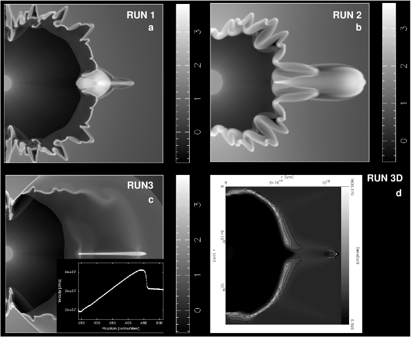
Figure 3: Logarithmically scaled density cuts through axisymmetrical simulations are shown. Panel ”a” shows a stagnation knot which expands significantly before escaping the rim of the PN, whereas in RUN 2 of panel ”b” it propagates about twice as far before reaching a similar expansion and has escaped the main PN. In panel ”c” a ”butterfly”-type PN is formed with a stagnation jet along the symmetry axis. The inset is a plot of the velocity of the gas on the axis given in units of cm/s. Note the linear increase in velocity as a function of distance in the region of the dense axial jet. Panel ”d” shows the 3D-simulation with the stagnation knot escaping the rim of the PN in a similar fashion as it does in the cylindrical 2D-runs.

	RUN 1	RUN 2	RUN 3	RUN 3D
Time	1190	1164	604	4053
WIND
$v_{0}$	1000	700	1000	1000
$n_{0}$	50	50	50	40
$\epsilon$	0.5	0.2	0.5	0.5
$\kappa$	2	2	2	2
$\theta_{0}$	50	30	20	20
ENV.
$n_{0}$	4000	2000	3500	240
$r_{0}$	8	5	5	8
$q$	0.2	0.5	0.2	1
$\delta$	4	4	4	4
$\alpha$	1.95	1.95	1.95	0

Table 1: The model parameters are given as used in equations 1 and 2. The units are as follows: time in years, velocity $v$ in ${\rm\ km\ s}^{-1}$, density $n_{0}$ in amu cm^-3, the angle $\theta$ in degrees, and the fiducial radius $r_{0}$ in units of $10^{16}$cm. Other quantities have no units. The cut-off time of the stellar wind is $4\times 10^{9}$ sec in all cases.

References

- (1) Aller, L.H. 1941, ApJ, 93, 236
- (2) Balick, B., Rugers, M., Terzian, Y., Chengalur, J. N. 1993, ApJ, 411, 778
- (3) Balick, B., Alexander, J., Hajian, A.R., Terzian, Y., Perinotto, M., Patriarchi, P. 1998, AJ, 116, 360
- (4) Biro, S., Raga, A.C., Cantó, J. 1995, MNRAS, 275, 557
- (5) Bobrowsky, M., Sahu, K. C., Parthasarathy, M., García-Lario, P. 1998, Nature, 392, 469
- (6) Bryce, M., López, J.A., Holloway, A.J., Meaburn, J. 1997, ApJ, 487, 161
- (7) Dopita, M.A. 1997, ApJ, 485L, 41
- (8) Cantó, J., Tenorio-Tagle, G., Róyczka, M. 1988, A&A, 192, 287
- (9) Cox, D.P., 1970, PhD Thesis (University of California, San Diego)
- (10) Dwarkadas, V.V.; Balick, B. 1998, ApJ, 497, 267
- (11) Frank, A., Balick, B., Livio, M. 1996, ApJ, 471L, 53
- (12) García-Segura, G., Langer, N., Róyczka, M. 1999, ApJ, 517, 767
- (13) García-Segura, G., López, J.A. 2000, ApJ, 544, 336
- (14) Goncalves, D.R., Corradi, R.L.M., Mampaso, A. 2000, ApJ, in press
- (15) Guerrero, M. A., Vázquez, R., López, J. A. 1999, AJ, 117, 967
- (16) Jones, T.W., Kang, H., & Tregillis, I.L. 1994, ApJ, 432, 194
- (17) Kahn, F., West, K. 1985, MNRAS, 212, 837
- (18) Kwok, S., Su, K.Y.L., Hrivnak, B.J. 1998, ApJ, 501, L117
- (19) Lim, A. 2001, MNRAS, submitted.
- (20) Lim, A., Steffen, W. 2001, MNRAS, 322, 166
- (21) López, J.A. 2000, RMxAC, 9, 201
- (22) Manchado, A., Guerrero, M., Stanghellini, L., Serra-Ricart, M. 1996, The IAC Morphological Catalog of Northern Galactic Planetary Nebulae, (La Laguna: IAC)
- (23) Meaburn J., Lopez, J.A., Noriega-Crespo, A. 2000, ApJSS, 128, 321
- (24) Moreno-Corral M.A, de la Fuente, E., Gutierrez, F. 1998, RevMexAA 34, 117.
- (25) O’Connor, J.A., Redman, M.P., Holloway, A.J., Bryce, M., López, J.A., Meaburn, J., 2000, ApJ, 531, 336
- (26) Peña, M., Hamann, W.-R., Koesterke, L., Maza, J., Mendez, R. H., Peimbert, M., Ruiz, M. T., Torres-Peimbert, S. 1997, ApJ, 491, 233
- (27) Peter, W., Eichler, D., 1995, ApJ, 438, 244
- (28) Petrenz, P., Puls, J. 2000, A&A, 358, 956
- (29) Raga, A.C., Taylor, S. D., Cabrit, S., Biro, S. 1995, MNRAS, 296, 833
- (30) Reay, N.K., Atherton, P.D. 1985, MNRAS, 215, 233
- (31) Redman, M.P., Dyson, J.E. 1999, MNRAS, 302, L17
- (32) Reimers, C., Dorfi, E.A., Höfner, S. 2000, A&A, 354, 573
- (33) Róyczka, M., & Franco, J. 1996, ApJ, 469, L127
- (34) Seaton, M. J. 1960, Report on Progress in Physics, 23, 313
- (35) Soker, N., Rappaport, S. 2000, ApJ, 538, 241
- (36) Soker, N., Regev, O. 1998, AJ, 116, 2462
- (37) Steffen, W., López, A.J. 1998, ApJ, 508, 696
- (38) Steffen, W., López, A.J. 2000, Asymmetrical Planetary Nebulae II: From Origins to Microstructures, ASP Conf. Series, Vol. 199, p. 413 Eds. J. H. Kastner, N. Soker, and S. Rappaport
- (39) van Leer, B. 1982, in Lecture Notes in Physics 170, Numerical Methods in Fluid Dynamics, ed. E. Krause, (Berlin: Springer), 507
- (40) Werner, K., Hamann, W.-R., Heber, U., Napiwotzki, R., Rauch, T., Wessolowski, U. 1992, A&A, 259L, 69