A Chandra X-ray Study of NGC 1068 — I. Observations of Extended Emission

Abstract

We report sub arc-second resolution X-ray imaging-spectroscopy of the archetypal type 2 Seyfert galaxy NGC 1068 with the Chandra X-ray Observatory. The observations reveal the detailed structure and spectra of the 13 kpc-extent nebulosity previously imaged at lower resolution with ROSAT. The Chandra image shows a bright, compact source coincident with the brightest radio and optical emission; this source is extended by $\simeq 1\farcs 5$ (165 pc) in the same direction as the nuclear optical line and radio continuum emission. Bright X-ray emission extends $\simeq 5\arcsec$ (550 pc) to the NE and coincides with the NE radio lobe and gas in the narrow line region. The large-scale emission shows trailing spiral arms and other structures. Numerous point sources associated with NGC 1068 are seen. There is a very strong correlation between the X-ray emission and the high excitation ionized gas seen in HST and ground-based [O iii] $\lambda 5007$ images. The X-rays to the NE of the nucleus are absorbed by only the Galactic column density and thus originate from the near side of the disk of NGC 1068. In contrast the X-rays to the SW are more highly absorbed and must come from gas in the disk or on the far side of it. This geometry is similar to that inferred for the narrow line region and radio lobes.

Spectra have been obtained for the nucleus, the bright region $\simeq 4\arcsec$ to the NE and 8 areas in the extended emission. The spectra are inconsistent with hot plasma models, the best approximations requiring implausibly low abundances ($\mathrel{\hbox to0.0pt{\lower 3.0pt\hbox{$\sim$}\hss}\raise 2.0pt\hbox{$<$}}0.1Z_{\odot}$). Models involving two smooth continua (either a bremsstrahlung plus a power-law or two bremsstrahlungs) plus emission lines provide excellent descriptions of the spectra. The emission lines cannot be uniquely identified with the present spectral resolution ($\sim 110$ – 190 eV), but are consistent with the brighter lines seen in the XMM-Newton RGS spectrum below 2 keV. Hard X-ray (above 2 keV) emission, including an iron line, is seen extending $\simeq 20\arcsec$ (2.2 kpc) NE and SW of the nucleus. Lower surface brightness, hard X-ray emission, with a tentatively detected iron line extends $50\arcsec$ (5.5 kpc) to the west and south. Our results, when taken together with the XMM-Newton RGS spectrum, suggest photoionization and fluorescence of gas by radiation from the Seyfert nucleus to several kpc from it. The facts that i) the large scale (arc minute) and small scale (few arc secs) X-ray emissions align well and ii) the morphology of the large-scale emission does not correlate well with the starburst suggests that the starburst is not the dominant source of the extended X-rays.

1 Introduction

Extended X-ray emission in Seyfert galaxies represents a potentially powerful probe of these active galactic nuclei. Such X-rays could originate from either a hot, collisionally-ionized or a much cooler photoionized gas. Both may plausibly be expected to be present in these objects. The narrow line regions of Seyferts are known to be the sites of mass motions of several hundreds to $\sim 1000\hbox{${\rm\thinspace km}{\rm\thinspace s}^{-1}\,$}$. Shocks associated with these motions will generate gas with temperatures $\simeq 10^{6}$ – $10^{7}$ K. Hot gas may also be present in the form of outflowing winds driven by radiation or radio jets from the nucleus. The compact, hard, UV – soft X-ray nuclear continuum source is believed to photoionize the narrow line region. Lines from highly ionized species, such as He ii, [Ne v], [Fe vii], [Fe x], [Fe xi] and [Fe xiv], are found in the optical and infrared spectra of these objects. X-ray lines from highly ionized species may, therefore, also be expected. High velocity shocks can also be powerful sources of ionizing radiation and, if present, should provide both collisionally- and photo-ionized gas. By searching for both of these components, X-ray observations can probe whether shocks are significant sources of ionizing radiation for the narrow line region. Extended X-ray emission can also arise through electron scattering and fluorescence of the nuclear radiation in extended gas. Morphological correspondences between the X-ray emitting gas and the optical line and radio continuum structures may provide clues to the nature of the X-ray emission.

For these reasons, we have begun a program of observing Seyfert galaxies with Chandra. Previous X-ray observatories have lacked the high spatial resolution ($\mathrel{\hbox to0.0pt{\lower 3.0pt\hbox{$\sim$}\hss}\raise 2.0pt\hbox{$<$}}1\arcsec$), wide energy coverage (0.1 – 10 keV) and good spectral resolution ($\sim 130{\rm\thinspace eV}$ from the CCD detectors) of Chandra. These capabilities are ideal for investigation of extended gas in Seyferts, and in this paper we present the results of observations of the nearby Seyfert 2 galaxy NGC 1068.

NGC 1068 was observed on three occasions with the Einstein observatory IPC by Monier & Halpern (1987). They found that the 0.1 – 4.5 keV spectrum could be described by a power law with energy index $\alpha=2.0\pm 0.3$ and absorbing column density consistent with the Galactic value. Combination of EXOSAT and Einstein IPC observations (Elvis & Lawrence, 1988) showed that the X-ray spectrum can be decomposed into two components — a steep low energy ($<2{\rm\thinspace keV}$) part with $\alpha=3.5$ and a flat high energy (2 – 10 keV) part with $\alpha\simeq 0.7$. This was the first detection in a Seyfert 2 of the hard power-law X-ray source known to be present in Seyfert 1s. Any intrinsic absorption was shown to be small ($N_{H}<3\times 10^{20}{\rm~{}atom~{}}\hbox{${\rm\thinspace cm}^{-2}\,$}$). Ginga observations (Koyama et al., 1989) confirmed the presence of the hard source above 2 keV, and also discovered an intense iron line with equivalent width $1.3\pm 0.1{\rm\thinspace keV}$, in accord with the predictions of Krolik & Kallman (1987). Marshall et al. (1993) obtained a higher spectral resolution (FWHM $\simeq 100{\rm\thinspace eV}$) observation with BBXRT. They found a total equivalent width for the Fe K line of 2.8 keV, and modeled the line profile in terms of three components corresponding to fluorescence of neutral (and lowly ionized) iron and recombination into both He-like and H-like iron. Fe L-shell emission was also detected. In a study with ASCA, Ueno et al. (1994) found emission from the H-like and / or He-like ions of Ne, Mg, Si and S and confirmed the Fe L and Fe K features found by Marshall et al. (1993). The best fit power-law spectrum above 3 keV has energy index $\alpha\simeq 0.3\pm 0.3$. Ueno et al. (1994) interpreted the steep low energy ($<3{\rm\thinspace keV}$) spectrum in terms of a two temperature (0.59 and 0.14 keV), optically-thin coronal plasma model. Iwasawa, Fabian & Matt (1997) reanalyzed the ASCA data, confirming the 3 components to the Fe K line complex which they interpreted with a model of cold and warm reflection. Netzer & Turner (1997) developed both photoionization and hot plasma models, including a hard reflected continuum. Their photoionized gas model is in good agreement with the emission lines observed by ASCA assuming solar metallicity for all elements except iron, which is more than twice solar, and oxygen, which is less than 0.25 solar. NGC 1068 has recently been studied with BeppoSAX. Matt et al. (1997) detected the galaxy in the 20 – 100 keV band, supporting models envisaging a mixture of both neutral and ionized reflections of an otherwise invisible nuclear source. The nucleus is completely obscured at all energies, implying it is “Compton-thick” — i.e. the column density of absorbing matter exceeds $N_{H}\sim 10^{25}{\rm~{}atoms~{}}\hbox{${\rm\thinspace cm}^{-2}\,$}$ (see also Matt et al. 2000). Soft X-ray spectroscopy with BeppoSAX (Guainazzi et al., 1999) reveals a spectrum rich in K$\alpha$ transitions of various elements below 3 keV.

The only X-ray image of NGC 1068 was obtained with the ROSAT HRI by Wilson et al. (1992) with $4\arcsec$ – $5\arcsec$ resolution. The observed X-ray emission could be divided into three components: i) an unresolved (radius $\leq 3\arcsec$) source associated with the Seyfert nucleus, ii) resolved circumnuclear (radius $<15\arcsec$) emission extending preferentially towards the NE and iii) large-scale ($15\arcsec<{\rm radius}<60\arcsec$) emission aligned NE-SW. Wilson et al. (1992) interpreted the circumnuclear emission as thermal emission from a nuclear wind and the large-scale emission as either associated with the disk starburst or an extension of the nuclear wind to larger radii. Further ROSAT HRI observations were reported by Wilson & Elvis (1997).

Very recently, Paerels et al. (2000) have reported a high spectral resolution observation of NGC 1068 with the XMM-Newton Reflection Grating Spectrometer. Their spectrum reveals a large number of emission lines below 2 keV. Based on the narrowness of the recombination radiation continua, the fact that the forbidden lines are stronger than the resonance lines in helium-like triplets, and the weakness of Fe L emission compared to Fe K emission, Paerels et al. (2000) conclude that the emission is dominated by recombination in cool X-ray photoionized gas. The N and O helium-like triplets may contain a $\mathrel{\hbox to0.0pt{\lower 3.0pt\hbox{$\sim$}\hss}\raise 2.0pt\hbox{$<$}}30\%$ component in collisional equilibrium.

The present paper is organized as follows. In section 2 we describe the observations and their reductions. Section 3 provides a brief discussion of the X-ray morphology, while section 4 presents the X-ray spectra obtained for the nucleus and five spatially extended regions. A comparison of the X-ray images with those in other wavebands is presented in section 5, and conclusions are given in section 6. Future papers will address the compact sources in the field and present a more detailed analysis of the extended emission.

NGC 1068 is at a heliocentric redshift of $z=0.00379$ (de Vaucouleurs et al., 1991) which, after correction to the frame of the microwave background and assuming $H_{0}=50\hbox{$\hbox{${\rm\thinspace km}{\rm\thinspace s}^{-1}\,$}{\rm\thinspace Mpc}^{-1}$}$ and $q_{0}=0$, corresponds to 22.8 Mpc, so $1\arcsec$ is equivalent to 110 pc. The Galactic column density towards NGC 1068 is $N_{H}({\rm Gal})=2.99\times 10^{20}\hbox{${\rm\thinspace cm}^{-2}\,$}$ (Murphy et al., 1996)

2 Observations and Reduction

Since the nucleus of NGC 1068 is known to be a strong X-ray source, we were concerned that “pile-up” could affect the Chandra observations. In order to measure the Chandra count rate from the nucleus and circumnuclear regions, we first obtained a short observation (obsid 343) of NGC 1068 on 1999 December 9 using chip S3 (backside illuminated) of the Advanced CCD Imaging Spectrometer (ACIS; Garmire et al. 2000). Single exposures with a 0.1 s frame-time were alternated with two exposures with a 0.4 s frame-time, the total integration time being $\mathrel{\hbox to0.0pt{\lower 3.0pt\hbox{$\sim$}\hss}\raise 2.0pt\hbox{$<$}}1$ ks. This observation showed that the nucleus is significantly piled up in the 0.4 s frame-time, but not in the 0.1 s frame-time. It also demonstrated that the count rate in the region extending $\simeq 6\arcsec$ NE from the nucleus is so high that data obtained from this region with the default frame-time of 3.2 s would be piled up, but data obtained with a 0.4 s frame-time would not be piled up. On this basis we decided to observe NGC 1068 for separate, longer exposures in all of 0.1 s, 0.4 s, and 3.2 s frame-times. The longer 0.1 s, 0.4 s and 3.2 s frame-time observations were thus designed to study primarily the X-ray emission of the nucleus, the extended region to the NE of the nucleus and the larger scale emission, respectively.

These longer integrations were taken with the ACIS instrument in two separate observations. On 2000 February 21 the standard 3.2 s frame-time was used. CCDs I2, I3, S1, S2, S3 and S4 were read out, though all of the detected X-ray emission from NGC 1068 is on S3. On 2000 February 22 the readouts were alternated between one 0.1 s and two 0.4 s frame-times in order to mitigate the effects of pile-up in the inner regions, as discussed above. The data were screened for times of high background count rates and aspect errors in the usual way. The 3.2 s, 0.4 s and 0.1 s frame-time data have total good exposure times of 47016.2 s, 11465.4 s and 1433.2 s, respectively. The “livetimes” for the alternating mode exposures were given incorrectly in the header and had to be computed separately. A corrected formula for the exposure time (G. Allen, private communication) was used, and the resulting livetimes are equal to the frame-time multiplied by the number of exposures taken with that frame-time.

Spectra and instrument responses were generated using ciao v1.1.5 and analyzed with xspec v11.0.1. Spectra were grouped to have at least 25 counts per energy bin to ensure that the $\chi^{2}$ fitting of the data was valid. When extracting spectra from complex regions the backscal keyword (equal to the fractional area of the chip occupied by the extraction region) was computed by hand, as the values generated by ciao are often incorrect.

In the absence of the gratings, X-ray spectra from CCD detectors such as ACIS are not invertible, i.e. one cannot uniquely determine the X-ray spectrum from the observed counts. To model such data the following technique is used. A parameterized model of the source spectrum is computed and folded through the instrument response. The folded model and data are then compared using, e.g., the $\chi^{2}$ test. Parameters of the model spectrum are adjusted to minimize the $\chi^{2}$ difference between the folded model and the data. The error bars for a single parameter are given by the range over which that parameter may be varied with $\Delta\hbox{$\chi^{2}$}=2.706$, keeping the other model parameters fixed. This is equivalent to the 90 per cent confidence interval for a single interesting parameter.

The backside illuminated S3 chip has a high sensitivity to very soft X-rays and significant counts at $\sim 0.1{\rm\thinspace keV}$ were seen from all regions. However the instrument response is uncertain below 0.50 keV, and this uncertainty increases towards lower energies. We thus restricted our modeling to photon energies above 0.25 keV.

2.1 Nucleus

Counts were extracted from a 3$\farcs$75 diameter circle centered on the nucleus. The 3.2 s frame-time data are extremely piled up and cannot be used for spectral fitting. In the 0.4 s frame-time data there are 25251 counts corresponding to a count rate of $2.20\pm 0.014$ ct${\rm\thinspace s}^{-1}\,$. In the 0.1 s frame-time data there are 4760 counts corresponding to a count rate of $3.32\pm 0.048$ ct${\rm\thinspace s}^{-1}\,$. The difference in count rate is due, in part, to the presence of pile-up in the 0.4 s frame-time data. The background is negligible in both this and the NE region.

2.2 NE Region

Counts were extracted from a 4$\farcs$1 $\times$ 4$\farcs$6 rectangle with longer length in position angle (PA) = $45^{\circ}$ centered on the extended emission 4$\farcs$25 to the NE of the nucleus. This region does not overlap with the region used to extract the spectrum of the nucleus. In the 3.2 s frame-time data there are 26871 counts corresponding to a count rate of $0.57\pm 0.003$ ct${\rm\thinspace s}^{-1}\,$. In the 0.4 s frame-time data there are 10069 counts corresponding to a count rate of $0.88\pm 0.01$ ct${\rm\thinspace s}^{-1}\,$. In the 0.1 s data there are 1349 counts corresponding to a count rate of $0.94\pm 0.03$ ct${\rm\thinspace s}^{-1}\,$. Thus, there is significant pile-up in the 3.2 s frame-time data in this region.

2.3 Larger Scale Emission

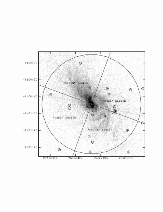
Figure 1: The extraction regions of the larger scale emission superposed on a grey scale image derived from the 3.2 s frame time data. Excluded point sources are indicated by circles.

The distribution and spectrum of larger scale emission was investigated with the 3.2 s frame-time data. The large scale region was divided into four quadrants with position angles $250^{\circ}\rightarrow 340^{\circ}$ (quadrant A), $340^{\circ}\rightarrow 70^{\circ}$ (quadrant B), $70^{\circ}\rightarrow 160^{\circ}$ (quadrant C) and $160^{\circ}\rightarrow 250^{\circ}$ (quadrant D). Position angle $\sim 25^{\circ}$, the bisector of quadrant B, corresponds to the approximate position angles of the radio emission and narrow line regions to the NE of the nucleus. Extraction regions between nuclear distances of $5\arcsec$ and $60\arcsec$ within quadrants A, B, C and D are termed the “West”, “North”, “East” and “South” regions respectively, and are shown in Figure 1. Obvious point sources determined by eye were excluded. Pile-up is not significant in any of these regions.

It is difficult to determine the spectrum of the background for the larger scale emission as there are no source-free regions nearby. To overcome this problem, we used a compilation of observations of relatively blank fields, from which discrete sources have been excised. For a particular source extraction region, a corresponding background region is taken from this compilation. The two regions have the same physical location on the S3 chip. The background images and software of Maxim Markevitch were used for this procedure.

3 X-ray Morphology

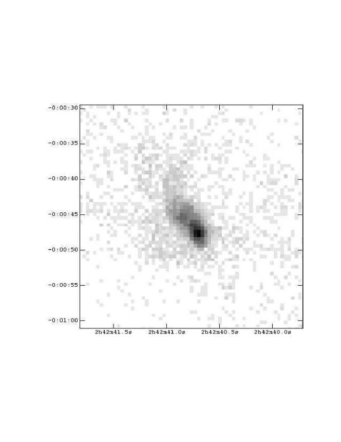
Figure 2: A grey scale representation of the Chandra X-ray image of NGC 1068 in the 0.25 – 7.50 keV band taken with a 0.1 s frame-time. Coordinates are for epoch J2000.0, both here and in subsequent Figures.

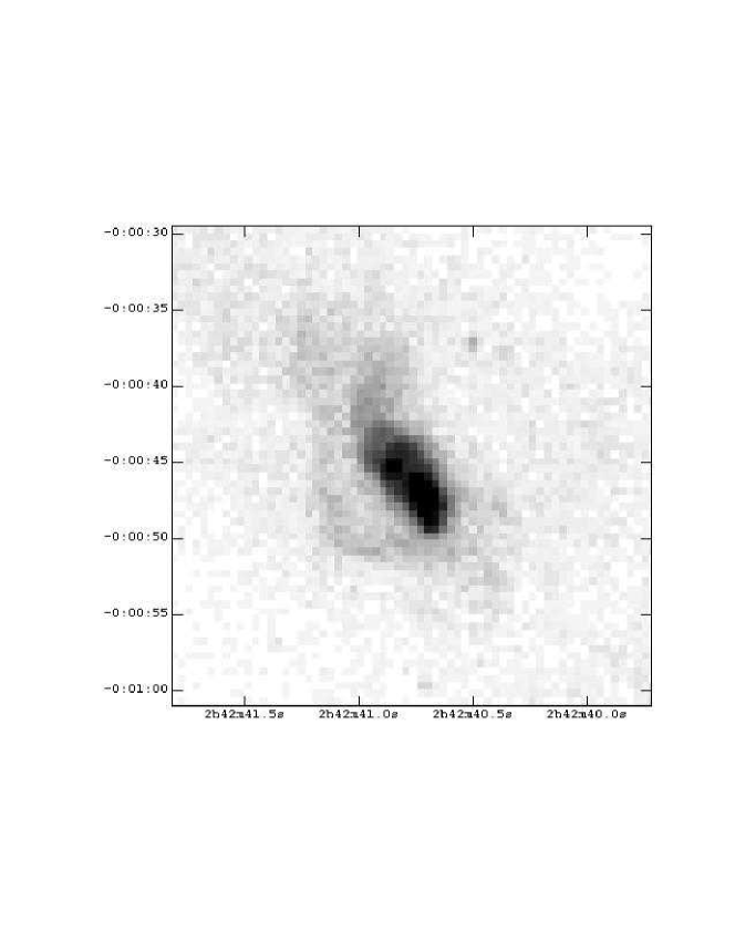
Figure 3: A grey scale representation of the Chandra X-ray image of NGC 1068 in the 0.25 – 7.50 keV band taken with a 0.4 s frame-time.

Grey scale images of the 0.1 s and 0.4 s frame-time Chandra X-ray observations of NGC 1068 are shown in Figures 2 and 3 respectively. The brightest region, which we refer to as the nucleus, extends $\simeq 1\farcs 5$ to the NE. Somewhat fainter X-ray emission extends $\simeq 6\farcs 5$ NE of the nucleus in PA $\sim 35^{\circ}$ – $40^{\circ}$, and perpendicular to this direction from 2$\farcs$5 SE to 2$\farcs$5 NW of the nucleus. There is a second peak of emission 3$\farcs$5 to the NE of the nucleus, with a brightness equal to approximately 15 per cent of the nucleus; this peak lies within the “NE region” (see section 2.2).

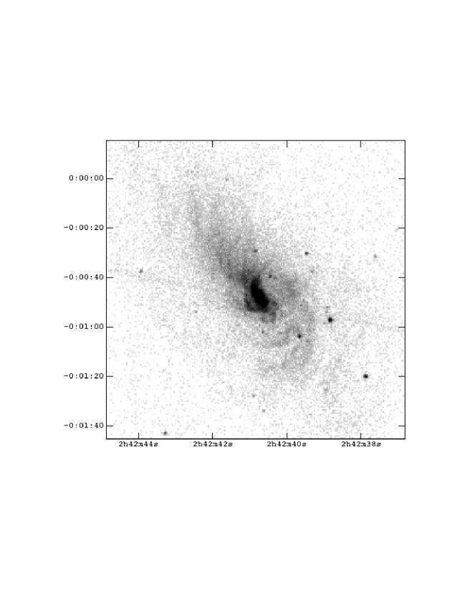
Figure 4: A grey scale representation of the Chandra X-ray image of NGC 1068 in the 0.25 – 7.50 keV band taken with a 3.2 s frame-time. The linear feature running from PA $78^{\circ}$ across the nucleus to PA $258^{\circ}$ is an instrumental effect.

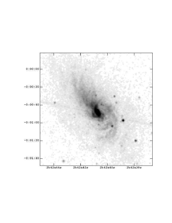
Figure 5: A grey scale representation of the Chandra X-ray image of NGC 1068, taken with a 3.2 s frame-time and smoothed by a Gaussian of $\sigma=0\farcs 5$. The linear feature running from PA $78^{\circ}$ across the nucleus to PA $258^{\circ}$ is an instrumental effect.

A grey scale image of the 3.2 s frame-time observation is shown in Figure 4. This image agrees well with the ROSAT HRI image (Wilson et al., 1992) when allowance is made for the lower resolution ($4\arcsec$ – $5\arcsec$) of the latter. Two bright “prongs” of X-ray emission extend from the bright region around the nucleus. One extends from the northern tip along PA $330^{\circ}$ for 7$\farcs$5, and the second extends from the southern tip along PA $90^{\circ}$ for 6$\farcs$5 before turning to follow PA $5^{\circ}$ for 4″. Significant extended X-ray emission is seen out to at least $60\arcsec$ to the NE, $50\arcsec$ to the SW, $20\arcsec$ to the NW and $30\arcsec$ to the SE of the nucleus. The most obvious large scale structures appear to be “spiral arms” that curve to lower PA with increasing radius from the nucleus, i.e. they are “trailing” arms. They may also be seen in an image of the 3.2 s frame-time data that has been smoothed by a Gaussian of $\sigma=0\farcs 5$ (Figure 5). The images also show many point sources of X-ray emission associated with NGC 1068.

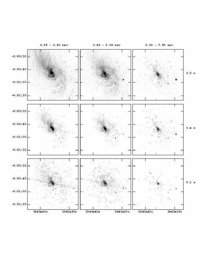
Figure 6: Grey scale representations of Chandra X-ray images of NGC 1068 in three energy bands and for each of the frame-times used. The top row has a 3.2 s frame-time, the center row 0.4 s frame-time and the bottom row 0.1 s frame-time. In the left column the energy range is 0.25 – 0.80 keV, the center column 0.80 – 2.00 keV and the right column 2.00 – 7.50 keV.

The X-ray morphologies in the 0.25 – 0.80 keV, 0.80 – 2.00 keV and 2.00 – 7.50 keV bands are shown in Figure 6, for the 0.1 s, 0.4 s and 3.2 s frame-time observations. The 0.25 – 0.80 keV X-ray emission has the greatest spatial extent, covering the range described above. The nucleus, NE region, the two “prongs” and the trailing arms are clearly seen. Only a few point sources, however, appear in these soft X-ray images. In the 0.80 – 2.00 keV energy band, there is still significant emission out to tens of arc-seconds, and many more point sources are visible. In the hardest energy band, 2.00 – 7.50 keV, emission extends at least $\sim 13\arcsec$ to the NE and SW of the nucleus and at least $\sim 4\arcsec$ to the NW and SE. The two “prongs” (to the N and E) do not stand out in hard X-rays, perhaps because of the lower sensitivity in this band. As the point spread function (PSF) at the location of the nucleus is circularly symmetric the observed, elongated extended hard X-rays are real. In addition, many hard point sources are clearly seen $\sim 20\arcsec$ from the nucleus.

4 X-ray Spectra

4.1 Nucleus

4.1.1 Thermal Plasmas

Initially the X-ray spectrum of the nucleus was modeled as an absorbed hot plasma with solar metal abundances. We used the “mekal” model (Mewe et al., 1985, 1986; Kaastra, 1992; Liedahl et al., 1995; Arnaud & Rothenflug, 1985; Arnaud & Raymond, 1992), which is included in the X-ray spectral fitting software xspec. The 0.1 s frame-time data were used as these do not suffer from pile-up. The model does not fit the data (see table 1), so a single hot plasma may be ruled out. Such plasmas overproduce iron L emission lines (i.e. transitions to the $n=2$ level) between 0.7 – 1.2 keV, and underproduce the high energy continuum above a few keV. A better fit is obtained if the metal abundances are allowed to vary, but the best fit value of zero is implausible for the nucleus of a spiral galaxy.

A model consisting of two hot plasmas, with temperatures of 0.17 keV and 0.73 keV and metal abundances of 3.0 per cent of solar and 2.7 per cent of solar respectively, provides an adequate description of the spectrum below 2 keV ($\hbox{$\chi^{2}$}=139$ for 74 degrees of freedom (d.o.f.)) Again, such low metal abundances are unlikely to be found in the inner regions of a spiral galaxy, so multiple hot plasma models are implausible for the nucleus of NGC 1068.

4.1.2 Bremsstrahlung Plus Power Law Plus Emission Lines

Many lines are seen below 1 keV in the XMM-Newton RGS spectrum (Paerels et al 2000), but these are confused by the limited spectral resolution of the Chandra ACIS spectrum reported here. Individual lines are sufficiently narrow to be unresolved by ACIS. We therefore decided to take a more phenomenological approach, modeling the data by a continuum plus individual emission lines. Firstly the continuum was described by a smooth model consisting of a bremsstrahlung plus a power law, both absorbed by the Galactic column. The residuals between the data and this smooth model were inspected by eye. Emission lines were then added to the model at energies expected to reduce the value of $\chi^{2}$. The energy and flux of these lines were free parameters. This process was repeated, adding lines until either an acceptable fit was achieved, or no further improvement was possible. Finally, our observed line energies were compared with those of the XMM-Newton RGS spectrum (a hard copy of which was kindly provided by F. Paerels) and, if agreement found, identified with lines therein.

The 0.1 s frame-time data are well described by a 0.45 keV bremsstrahlung plasma plus a hard power law of photon index $\Gamma=1.01^{+0.86}_{-1.15}$ plus a number of narrow emission lines, all absorbed by the Galactic column (last model in table 1). The spectrum and best fitting model are shown in Figure 7 and the emission lines are listed in table 2. Radiative recombination continua (RRC) are due to free-bound transitions from energy levels just above the ionization threshold; hence these lines start at the ionization threshold energy, and extend to higher energies (e.g. Paerels et al. 2000).

Our spectrum below 2 keV is generally consistent with lines seen in the XMM-Newton RGS spectrum (Paerels et al., 2000). The lines near and above 2 keV cannot be uniquely identified but are well described by neutral, hydrogen-like or helium-like lines of Si, S or Ar, with the exception of lines between 6.40 and 6.97 keV attributed to Fe. The Fe line complex is well described by a neutral Fe line with an equivalent width of 2.24 keV, although it should be noted that the true level of the continuum at the iron line energy is difficult to determine. The iron line is better resolved in the 0.4 s frame time data (see below). In view of the low signal-to-noise ratio, the line flux densities are quite uncertain.

The best fitting model has an unabsorbed 0.5 – 2.0 keV flux of $5.8\times 10^{-12}\hbox{${\rm\thinspace erg}{\rm\thinspace cm}^{-2}{\rm\thinspace s}^{-1}\,$}$ corresponding to an unabsorbed rest frame 0.5 – 2.0 keV luminosity of $3.6\times 10^{41}\hbox{${\rm\thinspace erg}{\rm\thinspace s}^{-1}\,$}$ and an unabsorbed 2.0 – 10.0 keV flux of $3.8\times 10^{-12}\hbox{${\rm\thinspace erg}{\rm\thinspace cm}^{-2}{\rm\thinspace s}^{-1}\,$}$ corresponding to an unabsorbed rest frame 2.0 – 10.0 keV luminosity of $2.3\times 10^{41}\hbox{${\rm\thinspace erg}{\rm\thinspace s}^{-1}\,$}$. The 2.0 – 10.0 keV flux and luminosity will have fractional errors comparable to the power law component of the model, listed in table 1.

The 0.4 s frame-time observation of the nucleus suffer from pile-up and it is difficult to determine the true shape of the continuum and the individual line fluxes. A recent model by Davis (2001), which is included as part of the Interactive Spectral Interpretation System (ISIS), includes effects of pile up in modeling spectra. We fitted the same spectral model to the 0.4 s frame-time data as was used to describe the 0.1 s frame-time data, with the continuum parameters allowed to vary and the emission line parameters fixed. The residuals between the data and this model were examined by eye and any clear discrepancies noted. The fluxes of model lines at energies near such discrepancies were then allowed to vary in an attempt to improve the fit. If this did not provide a satisfactory improvement, the line energy was also allowed to vary. If no model line existed near an obvious feature a new line was added. The reduced $\chi^{2}$ values for these overall fits were not as good as those for the 0.1 s frame-time data because we kept most of the line parameters fixed, even though very small changes may have improved the agreement between data and model. The pile-up fraction was estimated to be 22 per cent, and the continuum parameters ware close to those found for the 0.1 s frame-time data; the bremsstrahlung component was 0.1 keV warmer, and the power law component was slightly harder (but within the 0.1 s frame-time error bars) than the parameters derived from the 0.1 s frame-time observations. These small discrepancies are probably a result of imperfect modeling of the pile-up.

Emission-line fluxes from the 0.4 s frame-time observation are listed in the lower portion of Table 2. Note that the line fluxes tabulated for the 0.4 s frame time are the new total fluxes of those lines that have changed or been added, and are not the difference in line flux between the 0.1 s and 0.4 s frame-time observations. The 0.4 s differ from the 0.1 s results in that: i) the O viii RRC line is stronger (significantly above the 0.1 s frame-time error bars), ii) an Al line at 1.72 keV is probably present, iii) an “absorption” feature is seen at 1.54 keV that coincides with a sudden change in the effective area of the telescope, and is therefore probably caused by pile-up, iv) the Ar line better describes the data if it is shifted to 2.97 keV, and v) the Fe line is resolved into a neutral (6.4 keV) and ionized component ($\sim 6.80$ keV), the normalization of their sum being consistent with the single Fe line seen in the 0.1 s frame-time data. The fluxes of the neutral and ionized components are comparable.

4.2 NE Region

The 0.4 s frame-time data do not suffer from pile-up in the NE region, and have been used to determine both the shape of the continuum and the emission lines present. The 3.2 s data suffer from pile-up but have a higher signal-to-noise ratio and have been used where possible to investigate the X-ray emission lines, especially at higher energies.

4.2.1 Thermal Plasmas

The 0.4 s frame-time observations of the NE region were initially modeled by an absorbed hot thermal plasma with solar metal abundances, using the mekal model in xspec. The mekal model does not provide a good description of the data (see table 3) and may be ruled out. The model overproduces emission lines between 0.7 and 1.2 keV due to transitions to the L-shell of iron ions, and underproduces the high energy continuum above a few keV. The addition of a second hot thermal plasma with solar metal abundance improves the quality of the fit but again does not provide a good description of the spectrum (table 3).

4.2.2 Bremsstrahlung Plus Emission Lines

To further investigate the emission lines in the spectrum, the continuum was modeled by a smooth function consisting of two thermal bremsstrahlung components absorbed by the Galactic column. No physical meaning should be attributed to such a model, as an absorbed bremsstrahlung plus a power law model could have been used instead. Repeating the technique used to fit the spectrum of the nucleus, narrow emission lines were then added to the model. The XMM-Newton RGS spectrum (Paerels et al. 2000) was again used as a guide for the identification of the soft X-ray lines. As noted above, the spectral resolution of the ACIS is too low to provide unique identifications of the soft X-ray emission lines, many of which are blended together in our data below 1 keV. Two bremsstrahlung components with temperatures of 0.39 keV and 2.84 keV plus the stronger emission lines seen by Paerels et al. (2000) and a line at 2.38 keV, all absorbed by the Galactic column provides a good description of the spectrum with a $\chi^{2}$ of 78 for 62 d.o.f. (bottom model, table 3). The emission lines are listed in table 4, and the spectrum and model are shown in Figure 8.

A single data bin at 0.5 keV (see Figure 8) contributes significantly to the $\chi^{2}$ of the fit and, if removed, the quality of fit is improved to $\hbox{$\chi^{2}$}=65$ for 61 d.o.f. This data point is $9\sigma$ higher than its two neighbors over an energy range of 15 eV (Figure 8). This is much narrower than the instrumental response and the reason for this feature is unknown.

The line observed in the ACIS spectrum at 0.68 keV falls in the gap between strong lines of O viii Ly $\alpha$, Fe xvii and the radiative recombination continua of N vii and O vii seen in the RGS spectrum, and has been attributed to a blurred combination of these. The line at an observed energy of 0.76 keV is close to O viii Ly $\beta$ seen in the RGS spectrum, and has been attributed to this transition. The small discrepancy in line energy may result from blending with the RRC of O vii at 0.74 keV. The line at 1.00 keV falls between strong lines of Fe xx and Ne x seen in the RGS spectrum and may represent a combination of these. The weak line at 2.38 keV corresponds to the K$\alpha$ transition of sulphur in the ionization range S x – S xiv.

The best fit model to the 0.4 s frame-time data has an unabsorbed 0.5 – 2.0 keV flux of $1.6\times 10^{-12}\hbox{${\rm\thinspace erg}{\rm\thinspace cm}^{-2}{\rm\thinspace s}^{-1}\,$}$, corresponding to an unabsorbed rest frame 0.5 – 2.0 keV luminosity of $1.0\times 10^{41}\hbox{${\rm\thinspace erg}{\rm\thinspace s}^{-1}\,$}$, and an unabsorbed 2.0 – 10.0 keV flux of $2.0\times 10^{-13}\hbox{${\rm\thinspace erg}{\rm\thinspace cm}^{-2}{\rm\thinspace s}^{-1}\,$}$, corresponding to an unabsorbed rest frame 2.0 – 10.0 keV luminosity of $1.2\times 10^{40}\hbox{${\rm\thinspace erg}{\rm\thinspace s}^{-1}\,$}$.

The 3.2 s frame-time data suffer from pile-up so we followed the same procedure as was used for the 0.4 s frame-time observation of the nucleus. The pile-up fraction was estimated to be 46 per cent, but this is uncertain since the extraction region is not a point-source, as was assumed in modeling the pile-up. The continuum parameters are different to those found for the 0.4 s frame data; the cooler bremsstrahlung component is 0.1 keV warmer, and the hotter bremsstrahlung is 6.5 keV warmer. The significantly higher temperature of the latter component may be a result of the larger energy range of the 3.2 s frame-time data — i.e. the continuum model is required to produce significant X-ray flux at higher energies. The emission line fluxes from the 3.2 s frame-time data are listed at the bottom of Table 4. Again, note that the tabulated line fluxes are the total line fluxes and not the differences in flux between the 3.2 s and 0.4 s frame-time data. The changes are as follows: i) the N vii line has a preferred energy of 0.54 keV which corresponds to a sudden change in the effective area of the telescope, and is therefore probably caused by pile-up, ii) the Ne ix triplet is stronger, iii) the Ne ix He $\beta$ line is weaker, and iv) an Fe line is tentatively detected, but its energy is poorly constrained,

4.3 Larger Scale Emission

4.3.1 Thermal Plasmas

We followed a similar procedure to that used for the nucleus and NE region, applying it to the West, North, East and South regions in turn. The 3.2 s frame-time observations were used as they have the longest exposure time and do not suffer from pile-up. A hot plasma absorbed by the Galactic column does not provide a good description of the data from any of these regions, even if the metal abundances are allowed to vary (see table 5). The preferred values of the metal abundances are very low (less than 12 per cent solar), and the thermal model does not fit the significant hard X-ray emission seen from each region above 2 keV. We conclude that a single temperature thermal plasma model, absorbed by the Galactic column, cannot describe the spectrum in any of the larger scale extended regions.

4.3.2 Bremsstrahlung Plus Power Law Plus Emission Lines

The phenomenological approach described in section 4.1.2 was again used to study the emission lines from each of these regions. The continuum was described by a smooth model consisting of a bremsstrahlung plus power law, both absorbed by the Galactic column, to which individual emission lines were then added. The parameters of the continuum fits are listed in table 5, and the emission lines listed in tables 6 (West), 7 (North), 8 (East) and 9 (South). The spectrum and models are shown in Figures 9 (West), 10 (North), 11 (East) and 12 (South). Good fits were obtained with bremsstrahlung components with temperatures in the range 0.36 – 1.06 keV and power laws with photon indices in the range $\Gamma=-0.21$ to $0.92$, with the harder (lower) photon indices in the South and East regions. There is significant hard X-ray emission above 2 keV from each region, and an iron line is seen from the West, North and South regions. The unabsorbed broad-band fluxes and luminosities are listed in Table 10.

The energy dependent PSF of the Chandra mirrors will scatter a fraction of the flux from the nucleus and NE region over tens of arc-seconds and this can significantly contaminate the spectra of the larger scale extended emission regions. In particular, the wings of the PSF are stronger at higher energies and it is important to assess the reliability of the hard X-ray emission seen on the larger scales. Firstly, the spectra show hard ($\mathrel{\hbox to0.0pt{\lower 3.0pt\hbox{$\sim$}\hss}\raise 2.0pt\hbox{$>$}}3{\rm\thinspace keV}$) X-ray fluxes differing by a factor of $\sim 3-4$ between the East (the weakest) and South (the strongest) regions (see Figures 11 and 12 respectively). In the regions between $23\farcs 5$ – $60\arcsec$ a similar difference in hard X-ray flux is also seen (Figure 13), with stronger emission from the West and South. As the PSF is essentially circularly symmetric these must be due to differences in the intrinsic spectra of these regions. Secondly, images of the extended hard X-ray emission (e.g. Figure 6), are clearly not circularly symmetric with the strongest emission in the large-scale regions being seen in the South and West sectors.. This strongly suggests that scattering of nuclear emission by the circularly symmetric PSF cannot account for all of this emission. An “iron line” image was constructed by taking the 6.3 – 6.5 keV iron line band and subtracting normalized 5.8 – 6.3 and 6.5 – 7.0 keV continuum band images. The resulting distribution of discrete counts from the iron line extends $\sim 20\arcsec$ to the NE and SW, and at lower surface brightness $\sim 50\arcsec$ to the West and South. This agrees well with the hard X-ray flux and iron lines seen in the spectra of the extended and far-extended regions (Figures 9 – 12 and Figure 13).

To quantify the effects of scattering by the PSF the following approach was used. Four images were constructed in which the central circular region of radius $5\arcsec$ contained the observed distribution of emission in the bands 0.25 – 0.40, 1.10 – 1.90, 3.56 – 5.46 and 5.46 – 7.34 keV. Outside this radius (which corresponds to the inner border of the large-scale regions), the emission was set to zero. These images were then convolved with PSFs computed at 0.23, 1.50, 3.51 and 6.40 keV respectively, using the ciao tool mkarf. From the convolved images, the predicted count rate per keV due to telescope scattering from the inner bright region may be obtained for each of the larger scale extended regions. These are the four horizontal bars plotted in Figures 9 to 13. There is clear evidence of an excess of hard X-ray emission from the North and South regions, and tentative evidence from the West, whereas the hard X-ray flux from the East region may have been scattered from the nucleus by the telescope mirrors. Restricting our attention to the more distant regions between $23\farcs 5$ – $60\arcsec$ (Figure 13) we find there to be evidence of excess hard X-ray emission from the West and South regions, and possibly the North.

4.4 The Spatial Distribution of the Absorbing Column

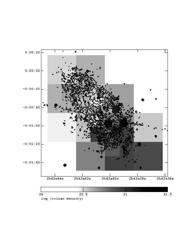
Figure 14: Contours of the 0.25 – 7.50 keV X-ray emission from the 3.2 s frame-time observation superposed on a map of the inferred absorbing column density to the soft X-ray emission (grey scale). Contours are plotted at 1, 2, 4, 8, 16, 32, 64, 128, 256 and 512 counts per pixel. The lowest contour levels are close to the noise, so counts have been averaged in blocks of $2\times 2$ pixels. The column density is seen to be larger to the SW of the nucleus than to the NE.

Spectra containing at least 800 counts were extracted from square regions of the 3.2 s frame-time Chandra data, allowing the absorbing column density to each region to be determined. Each spectrum was modeled by an absorbed mekal plasma with variable metal abundance over the energy range 0.25 – 3.00 keV. The resulting map of absorbing column density over the face of the galaxy is shown in Figure 14. The SW side of the galaxy shows absorption in excess of the Galactic column ($N_{H}({\rm Gal})=2.99\times 10^{20}\hbox{${\rm\thinspace cm}^{-2}\,$}$), whereas the NE side shows no significant excess absorption. This result shows that the extended X-ray emission to the NE of the nucleus is on the near side of the galactic disk of NGC 1068, while that to the SW is either in the galactic disk or on its far side. This geometrical arrangement agrees with indications from both the high excitation ionized gas seen at optical wavelengths and radio continuum observations. The ionized gas to the NE is much stronger than that to the SW, a difference usually attributed to excess obscuration on the SW side (e.g. Baldwin, Wilson & Whittle 1987; Evans et al. 1991). Further, the NE radio lobe is strongly polarized while that to the SW is unpolarized (Wilson & Ulvestad 1983, hereafter WU), consistent with the SW lobe being depolarized by gas in the galaxy disk. Lastly, H i 21 cm absorption observations indicate unambiguously that the NE radio lobe is located in front of the galaxy disk and the SW radio lobe is behind it (Gallimore et al., 1994).

5 Comparison with Observations in Other Wavebands

5.1 Registration of Images

NGC 1068 contains considerable structure within the central arc second. There are several radio components arranged in a “bent linear” structure (e.g. WU; Ulvestad, Neff & Wilson 1987; Muxlow et al. 1996; Gallimore et al. 1996, Gallimore, Baum & O’Dea 1997; Roy et al. 1998). There is also structure in optical emission line and continuum images obtained with HST (e.g. Evans et al. 1991; Macchetto et al. 1994), and in both near- and mid-infrared band images obtained at the diffraction limit of large ground-based telescopes (e.g. Weinberger, Neugebauer & Matthews 1999; Bock et al. 2000).

The location of the true nucleus (meaning the putative black hole and its accretion disk) has been much discussed. Radio source S1 has a flat or inverted spectrum (Gallimore et al. 1996), which may originate through thermal emission from the inner edge of the obscuring torus (Gallimore, Baum & O’Dea 1996; Roy et al. 1998). VLBA imaging (Gallimore, Baum & O’Dea 1997) shows that this source is a parsec-sized disk of ionized gas. Source S1 is also the location of water maser emission, indicative of dense molecular gas (Claussen & Lo 1986; Greenhill et al. 1996). To within measurement errors, radio source S1 is coincident with the peaks of mid-infrared (Braatz et al. 1993) and near-infrared (Thatte et al. 1997) light, and probably with the center of symmetry of the polarization pattern of scattered UV light (Capetti et al. 1995; Kishimoto 1999). There is thus a general consensus that these features mark the location of the true nucleus.

There is, however, no particular reason why the peak of X-ray emission should coincide with this location. The column density, N_H, to the X-ray nucleus of NGC 1068 exceeds $\sim$ 10²⁵ cm^-2 (e.g. Matt et al. 2000), so all of the X-ray emission we observe must be either intrinsically extended or scattered nuclear light. The Chandra astrometry is not currently accurate enough for a precise location of the nucleus with respect to the sub arc-second scale features described in the previous paragraph. The position of the peak of the broad-band X-ray emission, as measured by the 0.4s frame-time exposure, is: $\alpha_{\rm x}$(J2000) = 02^h 42^m 40$\fs$71, $\delta_{\rm x}$(J2000) = –00^∘ 00^′ 47$\farcs$7. This position is remarkably close to that of the brightest radio source in the nucleus at 5 GHz (Muxlow et al. 1996): $\alpha_{\rm r}$(J2000) = 02^h 42^m 40$\fs$715s, $\delta_{\rm r}$(J2000) = –00^∘ 00^′ 47$\farcs$64. The difference in each coordinate is $<$ 0$\farcs$1. This agreement is considerably better than expected given Chandra’s current absolute astrometric errors and may thus be coincidental. Nevertheless, we decided to align the peak in the Chandra image with the peak in a 5 GHz radio map with 0$\farcs$4 resolution (WU), which is similar to, though somewhat better than, the resolution of the Chandra image. Simulations showed that smoothing the 60 mas resolution 5 GHz map of Muxlow et al. (1996) to the 0$\farcs$4 resolution of the WU map moves the radio peak slightly to the NE (by $\leq$ 0$\farcs$1 in each coordinate) to: $\alpha_{\rm rs}$(J2000) = 02^h 42^m 40$\fs$721, $\delta_{\rm rs}$(J2000) = –00^∘ 00^′ 47$\farcs$55. This position agrees to $\leq$ 0$\farcs$1 with the actual position of the peak in the WU map after precessing the original B1950.0 coordinates of that map to J2000.0 using the facility in the ds9 display program.

Thus, for purposes of comparison with observations in other wavebands, the peak in the broad-band Chandra image was assigned the coordinates $\alpha_{\rm rs}$, $\delta_{\rm rs}$ given above. In order to extend the astrometric comparison to optical images, we used the alignment between the optical and radio emissions obtained by Capetti, Macchetto & Lattanzi (1997). These authors obtained absolute astrometry for the HST images by taking three images: a photographic refractor plate, a ground-based CCD image and an HST image. The plate covered astrometric standard stars from which astrometric positions were obtained for many fainter, secondary astrometric reference stars some of which are on the CCD image. Finally, the astrometric scale of the HST image was registered to the ground-based CCD image by a cross-correlation technique. From this procedure, the location of the peak of emission in the HST optical continuum (filter F547M) image is found to be: $\alpha_{\rm o}$(J2000) = 02^h 42^m 40$\fs$711, $\delta_{\rm o}$(J2000) = –00^∘ 00^′ 47$\farcs$81 (Capetti, Macchetto & Lattanzi 1997). This position is also very close to the Chandra-measured location of the X-ray peak: $\alpha_{\rm x}$ – $\alpha_{\rm o}$ = 0$\farcs$015, $\delta_{\rm x}$ – $\delta_{\rm o}$ = 0$\farcs$15, which represents agreement given the Chandra errors.

We emphasize that this astrometric registration between the X-ray image on the one hand and the radio and optical images on the other is not precise and may change as the Chandra astrometry improves. However, this uncertainty only affects the alignment on sub arc-second scales, such as is needed to compare the Chandra image with HST and radio interferometric data. Spatial comparisons on larger scales (i.e. $>$ 1^′′) are robust. In the following, we compare the X-ray morphology with that in the optical line, optical continuum and radio continuum.

5.2 Comparison with Optical Emission-Line Images

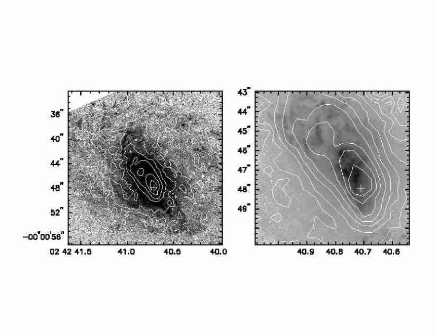
Figure 15: A superposition of the circumnuclear distribution of X-rays on an HST image taken through filter F502N (Dressel et al. 1997; Capetti, Axon & Macchetto 1997); this image is dominated by the light of [O iii] $\lambda$5007. The images were aligned as described in Section 5.1. The X-ray image (contours) represents photon events in the energy range 0.25 – 7.5 keV taken from the 0.4s frame-time observation at the full Chandra resolution. The cross marks the position of radio source S1, which is believed to coincide with the nucleus (Section 5.1). The right panel is an enlarged view of the circumnuclear region. Left panel: Contours are plotted on a logarithmic scale at log (cts pixel^-1) = 0.5, 1.0, 1.5, 2.0, 2.5 and 3.0. The greyscale is proportional to the square root of the intensity and ranges from 1 $\times$ 10^-18 (white) to 1 $\times$ 10^-16 (black) erg cm^-2 s^-1 (PC pixel)^-1. Right panel: Contours are plotted on a logarithmic scale at log (cts pixel^-1) = 0.3, 0.6, 0.9, 1.2, 1.5, 1.8, 2.1, 2.4, 2.7, 3.0. The greyscale is proportional to the logarithm of the intensity and ranges from 1 $\times$ 10^-17 (white) to 1 $\times$ 10^-13 (black) erg cm^-2 s^-1 (PC pixel)^-1. A close association is seen between many structures in the two wavebands.

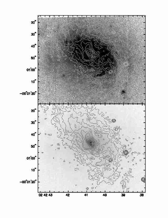
Figure 17: A superposition of the Chandra 3.2s frame-time data with events in the range 0.25 to 7.5 keV (contours) on an image in the velocity-integrated [O iii] $\lambda$5007 line (grey scale) taken with the Taurus Fabry-Perot instrument on the AAT (G. Cecil, private communication). The images were aligned as described in Section 5.1 and the cross marks the position of radio source S1, which is believed to coincide with the nucleus (Section 5.1). The “hole” at the nucleus in the X-ray image is not real but results from pile-up (Section 2). The X-ray image has been smoothed with a Gaussian function of standard deviation $\sigma$ = 0$\farcs$5. The resolution (seeing) of the [O iii] image is 1$\farcs$0 (FWHM), very similar to that of the smoothed Chandra image. The X-ray image is contoured at 1, 2, 4, 8, 16, 32, 64, 128, 256 and 512 cts (pixel)^-1 in both panels. The greyscale is proportional to the logarithm of the number of counts per pixel in both panels and the two panels differ only in the scaling of the grey scale. In the top panel, it ranges from log cts pixel^-1 = 0.5 (white) to 1.3 (black) and in the bottom from log cts pixel^-1 = 0.5 (white) to 4 (black).

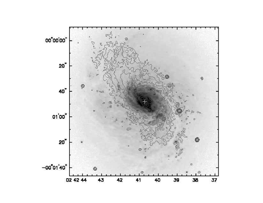
Figure 18: A superposition of the Chandra 3.2s frame-time data with events in the range 0.25 to 7.5 keV (contours) on an optical continuum image taken through a filter with center wavelength/bandwidth 6100/200 Å (grey scale; Pogge & De Robertis 1993). The images were aligned as described in Section 5.1 and the cross marks the position of radio source S1, which is believed to coincide with the nucleus (Section 5.1). The “hole” at the nucleus in the X-ray image is not real but results from pile-up (Section 2). The resolution of the optical image is 0$\farcs$5 – 0$\farcs$6. The Chandra image has been smoothed with a Gaussian function of standard deviation $\sigma$ = 0$\farcs$5 and is contoured at 1, 2, 4, 8, 16, 32, 64, 128, 256 and 512 cts pixel^-1. The grey scale of the optical image is proportional to the square root of the intensity between 1 (white) and 2000 cts pixel^-1 (black). Noteable correlations between the two images are apparent.

Figure 15 shows the X-ray emission (contours) superposed on an HST image taken through filter F502N; this image is dominated by [O iii] $\lambda$5007. There is remarkable agreement between the structures in the two wavebands. To the S of the nucleus (assumed to be radio source S1, marked by the cross) and within 2^′′ of it (Figure 15, right), the structure in both wavebands is aligned approximately N-S (PA $\simeq$ 13^∘) and there are detailed correspondences between the two images. To the N of the nucleus, both structures bend towards higher PA, reaching PA $\simeq$ 35^∘ some 4^′′ from the nucleus. It is notable that the bright extension of the X-rays corresponds closely to the bright emission-line clouds which extend from the nucleus to $\sim$ 2^′′ NE of it (Figure 15, right). There is also a close correspondence between the brightnesses slightly further (6^′′) from the nucleus, where the X-ray contours take a V-shaped form, with apex towards the NE (see also Figures 17 and 18).

Correspondences are also seen on the larger scale shown in Figure 15, left. Some 7^′′ NE of the nucleus, there is a prominent narrow feature in the HST image that first extends N and then curves towards the NW, ending up extending in PA $\sim$ 287^∘ when 10^′′ from the nucleus. The X-ray ridge, although observed with lower resolution, follows this feature closely. An arm-like feature in the HST image begins some 4^′′ SE of the nucleus and curves towards lower PA, extending towards the NE and ending up some 6 – 7 ^′′ E of the nucleus; the X-ray contours follow it closely. Various other close correspondences between the faint [O iii] and X-ray emission are also visible in Figure 15, left.

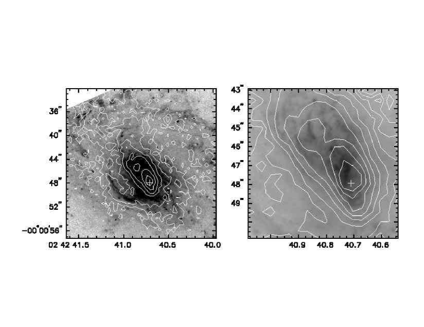
Figure 16: A superposition of the circumnuclear distribution of X-rays on an HST image taken through filter F658N (Dressel et al. 1997; Capetti, Axon & Macchetto 1997); this image is dominated by the light of H$\alpha$ + [N ii] $\lambda\lambda$6548, 6583. The images were aligned as described in Section 5.1. The X-ray image (contours), the contour levels and the cross are the same as shown in Figure 15. The right panel is an enlarged view of the circumnuclear region. Left panel: The greyscale is proportional to the square root of the intensity and ranges from 1 $\times$ 10^-18 (white) to 2 $\times$ 10^-16 (black) erg cm^-2 s^-1 (PC pixel)^-1. Right panel: The greyscale is proportional to the logarithm of the intensity and ranges from 1 $\times$ 10^-17 (white) to 1 $\times$ 10^-13 (black) erg cm^-2 s^-1 (PC pixel)^-1. As for the [O iii] $\lambda$5007 image (Figure 15), there are clear associations between structures in the two wavebands.

Similar correspondences are seen between the X-ray emission and the HST image through filter F658N (Figure 16), which is dominated by H$\alpha$ + [N ii] $\lambda\lambda$6548, 6583. The relative intensities of the various line features are different in this band (e.g. the narrow feature beginning 7^′′ NE is much weaker here than in [O iii]) but there is still a close association between the structures in the two wavebands.

A comparison between [O iii] $\lambda$5007 and X-ray emission on a larger scale is shown in Figure 17. The lower panel shows again the extension from the nucleus to the NE which is common to the two images. The overall shape of the outer X-ray contours is similar to the [O iii] (top panel). To the SW, there are two spiral arms that curve outwards in a clockwise sense (i.e. they trail the galactic rotation). The inner, brighter one is some 18^′′ and the outer, fainter one some 28^′′ from the nucleus. In both cases, there is a remarkably precise alignment with the X-ray contours (top panel). The stronger, X-ray point sources are not seen in the [O iii] image; this is not surprising if they are X-ray binaries in NGC 1068.

5.3 Comparison with Optical Continuum Images

Figure 18 shows the Chandra X-ray contours superposed on a red continuum image (from Pogge & De Robertis 1993). Features common to both images include a protrusion 7 – 8^′′ SW of the nucleus and, as described in the previous subsection, the two spiral arms SW of the nucleus and the arm-like feature SE and E of the nucleus. However, on the largest scales on which X-ray emission is seen, the X-ray image is much more elongated than the optical. There is little or no X-ray emission seen more than 30^′′ from the nucleus in the SE or NW directions, while the X-rays extend much further to NE and SW. The impression gained from these comparisons with optical data is that the X-rays correlate more strongly with the optical line than the optical continuum emission.

This absence of a close correlation between the X-ray and optical continuum images strongly suggests that the starburst disk is not the dominant source of the extended X-ray emission.

5.4 Comparison with Radio Continuum Images

As noted in Section 5.1, radio continuum images with sub arc-second resolution reveal a “bent linear” structure extending over 1$\farcs$5. Although the Chandra image of the central regions (e.g. Figure 15) does not have good enough resolution for a meaningful comparison, the extension of the X-ray emission immediately to the S of the nucleus is more or less N-S, like the radio emission. North of the nucleus, the X-ray ridge line “bends” towards the NE, as does the radio emission. Capetti, Macchetto & Lattanzi (1997) show that this arc second-scale radio structure lies in a region of relatively low optical line emission and is surrounded by emission line clouds. As argued by many authors (e.g. Wilson & Willis 1980; Wilson, Ward & Haniff 1988; Evans et al. 1991; Macchetto et al. 1994; Gallimore, Baum & O’Dea 1996), the structure of the narrow line region implies compression of interstellar gas by the radio ejecta. Thus, given the close association between the X-rays and the narrow line region (Section 5.2), the alignment between the X-rays and the arc second-scale radio structure is expected.

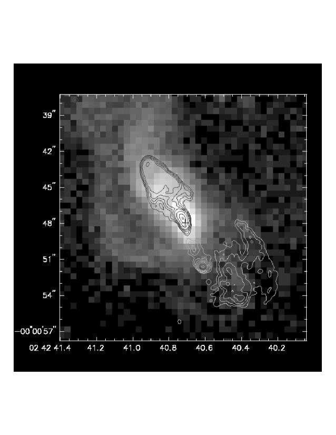
Figure 19: A superposition of the circumnuclear distribution of X-rays (grey scale) on a VLA 6 cm radio map (contours) with resolution 0$\farcs$38 $\times$ 0$\farcs$38 (Wilson & Ulvestad 1983). The images were aligned as described in Section 5.1. The X-ray image is the same as shown in Figure 3. The cross marks the position of radio source S1, which is believed to coincide with the nucleus (Section 5.1). Contours are plotted at 0.0005, 0.001, 0.002, 0.004, 0.008, 0.032, 0.128 and 0.256 Jy (beam)^-1. The greyscale is proportional to the logarithm of the X-ray intensity and ranges between log cts pixel^-1 = 0 (black) and 3.0 (white).

A comparison between the X-ray (grey scale) and radio (contours) images on a larger scale is shown in Figure 19. The V-shaped, edge-brightened radio lobe to the NE, which may represent a blast wave driven into the interstellar gas by the radio ejecta (Wilson & Ulvestad 1987), is seen to be associated with bright X-ray emission. The X-ray image also exhibits a V-shaped structure with apex some 6^′′ from the nucleus (see also Figures 15, 17). This structure is obviously connected with the radio “V”, but has a wider opening angle. This last difference may result, in part, from the lower resolution of the X-ray image. To the SW of the nucleus, the X-rays are much weaker, consistent with the higher absorbing column to the X-ray emitting gas found here (Section 4.4). Nevertheless, the brighter regions of radio emission in the SW lobe do appear to be associated with brighter X-ray emission. There is little or no enhancement of the X-ray emission at the radio “hot spot” 4$\farcs$0 SW of the nucleus.

6 Conclusions

We have obtained the highest resolution ($<1\arcsec$) image to date of the X-ray emission of NGC 1068. This image shows i) a bright nucleus close to or coincident with the brightest radio and optical emission, ii) bright emission extending $\simeq 5\arcsec$ (550 pc) to the NE, iii) large-scale structure reaching at least $1\arcmin$ (6.6 kpc) to the NE and SW, including X-ray emission from spiral arms, and iv) numerous point sources, most of which are likely to be associated with NGC 1068.

X-ray spectra have been obtained for ten regions – the nucleus, the bright region several arc-seconds to the NE, four $90^{\circ}$ sectors between $5\arcsec$ and $60\arcsec$ from the nucleus and four similar sectors between $23\farcs 5$ and $60\arcsec$ from the nucleus. Hot plasma models are poor descriptions of the spectra and the best approximations require implausibly low ($\mathrel{\hbox to0.0pt{\lower 3.0pt\hbox{$\sim$}\hss}\raise 2.0pt\hbox{$<$}}0.1Z_{\odot}$) abundances. We have constructed models of the spectra comprising two smooth continua (a bremsstrahlung plus a power-law or two bremsstrahlung spectra) plus emission lines. The lines cannot be uniquely identified with the present spectral resolution but are generally consistent with the stronger lines seen in the XMM-Newton RGS spectrum below 2 keV (Paerels et al., 2000). Above 2 keV we observe K$\alpha$ transitions of sulfur, argon and iron. Hard X-ray emission, including an iron line, is seen extending $\sim 20\arcsec$ (2.2 kpc) NE and SW of the nucleus. Lower surface brightness hard X-ray emission, with a tentatively detected iron line, extends $\sim 50\arcsec$ (5.5 kpc) to the west and south. Taken together with the XMM-Newton RGS spectrum, our results suggest photoionization and fluorescence of gas by radiation from the Seyfert nucleus to several kilo-parsecs from it.

An investigation of the distribution of absorbing column shows that the emission to the NE of the nucleus is absorbed by only the Galactic column and is thus on the near side of the disk of NGC 1068. The X-ray emission to the SW of the nucleus suffers greater absorption and must originate in or behind the disk of NGC 1068. This geometry agrees with that inferred for both the narrow line region observed at optical wavelengths and the radio ejecta.

We have compared the X-ray image with optical emission-line, optical continuum and radio continuum images. There is a very strong correlation between the X-ray emission and high excitation optical line emission (as traced by [O iii] $\lambda 5007$), consistent with photoionization in both wavebands. To the SW, the X-ray spiral arms correlate closely with those seen in [O iii] $\lambda 5007$. The NE radio lobe some $6\arcsec$ (660 pc) from the nucleus shows a strong morphological correlation with the X-ray emission, suggestive of interstellar gas being compressed by the radio ejecta. The alignment of the large-scale (arc min) and small scale (few arc sec) X-ray emissions and the lack of a close correlation between the larger scale X-ray emission and the optical continuum strongly suggests that the starburst is not the dominant source of these X-rays.

We plan to present a discussion of the compact X-ray sources seen in NGC 1068 and a more detailed analysis of the extended emission in future papers.

We thank the Chandra Science Center, especially Dan Harris and Shanil Virani, for assistance with the observations. Glenn Allen gave valuable advice on the alternating exposure mode. We are grateful to Gerald Cecil and Frits Paerels for providing data in advance of publication. We thank John Houck for assistance with ISIS. This research was supported by NASA grant NAG 81027.

Table 1: Spectral Fits to the Nucleus from 0.1 s Frame-Time Observation

Model	$N_{H}$	Temperature	Abundance	Photon index	Normalization	$\chi^{2}$ / d.o.f.
	[$\times 10^{20}\hbox{${\rm\thinspace cm}^{-2}\,$}$]	[ keV]	[$\times Z_{\odot}$]
MEKAL	2.99	0.65	1.0		$K_{\rm MEKAL}=1.6\times 10^{-3}$	2415 / 88
Brem	2.99	0.53			$K_{\rm Brem}=1.1\times 10^{-2}$	321 / 88
Brem + PL	2.99	0.46		0.83	$\left\{\begin{array}[]{c}K_{\rm Brem}=1.2\times 10^{-2}\\ K_{\rm PL}=2.0\times 10^{-4}\end{array}\right\}$	202 / 86
Brem + PL + lines	2.99	$0.45^{+0.03}_{-0.08}$		$1.01^{+0.86}_{-1.15}$	$\left\{\begin{array}[]{c}K_{\rm Brem}=\left(1.0^{+0.1}_{-0.1}\right)\times 10^{-2}\\ K_{\rm PL}=\left(2.3^{+3.4}_{-1.9}\right)\times 10^{-4}\end{array}\right\}$	67 / 64

Table 2: X-ray Spectral Lines From the Nucleus

Frame-time	Energy	Line	Observed energy	$K$
[sec]	[keV]		[keV]
0.1	0.37	C vi Ly $\alpha$	$0.34^{+0.02}_{-0.01}$	$\left(3.4^{+1.6}_{-1.9}\right)\times 10^{-4}$
0.1	0.43	N vi triplet	$0.42^{+0.01}_{-0.01}$	$\left(5.1^{+1.7}_{-1.9}\right)\times 10^{-4}$
0.1	0.56 – 0.57	O vii triplet	$0.56^{+0.01}_{-0.01}$	$\left(4.9^{+1.8}_{-1.2}\right)\times 10^{-4}$
0.1	$\left\{\begin{array}[]{c}0.73\\ 0.74\end{array}\right.$	Fe L xvii O vii RRC $\left.\begin{array}[]{c}\\ \\ \end{array}\right\}$	$0.74^{+0.01}_{-0.02}$	$\left(9.3^{+4.8}_{-5.3}\right)\times 10^{-5}$
0.1	0.87	O viii RRC	$0.86^{+0.02}_{-0.03}$	$\left(9.6^{+4.1}_{-5.9}\right)\times 10^{-5}$
0.1	0.90 – 0.92	Ne ix triplet	$0.92^{+0.03}_{-0.02}$	$\left(1.4^{+0.3}_{-0.6}\right)\times 10^{-4}$
0.1	1.02	Ne x Ly $\alpha$	$1.01^{+0.01}_{-0.02}$	$\left(7.6^{+3.0}_{-3.1}\right)\times 10^{-5}$
0.1	1.07	Ne ix He $\beta$	$1.11^{+0.02}_{-0.02}$	$\left(4.3^{+3.0}_{-3.1}\right)\times 10^{-5}$
0.1	1.33 – 1.34	Mg xi triplet	$1.31^{+0.04}_{-0.05}$	$\left(2.8^{+1.7}_{-1.9}\right)\times 10^{-5}$
0.1	1.84 – 1.86	Si xiii triplet	$1.84^{+0.03}_{-0.04}$	$\left(2.9^{+1.4}_{-1.4}\right)\times 10^{-5}$
0.1	2.31 – 2.35	S ii – S x	$2.30^{+0.03}_{-0.04}$	$\left(3.6^{+2.1}_{-2.1}\right)\times 10^{-5}$
0.1	2.96 – 3.00	Ar ii – Ar xi	$2.85^{+0.15}_{-0.06}$	$\left(1.8^{+1.3}_{-1.4}\right)\times 10^{-5}$
0.1	6.40 – 6.97	Fe ii – Fe xxvi	6.40	$\left(7.3^{+3.3}_{-3.3}\right)\times 10^{-5}$
0.4	0.87	O viii RRC	0.86	$2.2\times 10^{-4}$
0.4	—	Artifact	1.54	$-5.5\times 10^{-5}$
0.4	1.73	Al xiii Ly $\alpha$	1.72	$2.5\times 10^{-5}$
0.4	2.96 – 3.00	Ar ii – Ar xi	2.97	$1.8\times 10^{-5}$
0.4	6.40	Fe ii	6.40	$4.3\times 10^{-5}$
0.4	$\left\{\begin{array}[]{c}6.70\\ 6.97\end{array}\right.$	Fe xxv Fe xxvi $\left.\begin{array}[]{c}\\ \\ \end{array}\right\}$	6.80	$5.5\times 10^{-5}$

Table 3: Spectral Fits to the NE Region from the 0.4 s Frame-Time observation

Model	$N_{H}$	Temperature	Abundance	Normalization	$\chi^{2}$ / d.o.f.
	[$\times 10^{20}\hbox{${\rm\thinspace cm}^{-2}\,$}$]	[keV]	[$\times Z_{\odot}$]
MEKAL	2.99	0.63	1.0	$K_{\rm MEKAL}=5.1\times 10^{-4}$	4201 / 92
2 $\times$ MEKAL	2.99	$\left\{\begin{array}[]{c}0.21\\ 1.48\end{array}\right.$	$\begin{array}[]{c}1.00\\ 1.00\end{array}$	$\left.\begin{array}[]{c}K_{\rm MEKAL}=7.8\times 10^{-4}\\ K_{\rm MEKAL}=5.5\times 10^{-4}\end{array}\right\}$	1780 / 90
2 $\times$ Brem + lines	2.99	$\left\{\begin{array}[]{c}0.39^{+0.02}_{-0.05}\\ 2.84^{+0.95}_{-0.41}\end{array}\right.$		$\left.\begin{array}[]{c}K_{\rm Brem}=\left(2.5^{+0.2}_{-0.1}\right)\times 10^{-3}\\ K_{\rm Brem}=\left(1.2^{+0.8}_{-0.3}\right)\times 10^{-4}\end{array}\right\}$	78 / 62

Table 4: X-ray Spectral Lines From the NE Region

Frame-time	Energy	Line	Observed energy	$K$
[sec]	[keV]		[keV]
0.4	0.37	C vi Ly $\alpha$	$0.36^{+0.01}_{-0.01}$	$\left(7.6^{+2.4}_{-2.5}\right)\times 10^{-5}$
0.4	0.43	N vi triplet	$0.42^{+0.01}_{-0.01}$	$\left(1.0^{+0.3}_{-0.3}\right)\times 10^{-4}$
0.4	0.50	N vii	$0.52^{+0.00}_{-0.01}$	$\left(7.1^{+1.6}_{-1.5}\right)\times 10^{-5}$
0.4	0.59	N vii Ly $\beta$	$0.58^{+0.00}_{-0.00}$	$\left(1.1^{+0.2}_{-0.1}\right)\times 10^{-4}$
0.4	$\left\{\begin{array}[]{c}0.65\\ 0.67\\ 0.73\\ 0.74\end{array}\right.$	O viii Ly $\alpha$ N vii RRC Fe L xvii O vii RRC $\left.\begin{array}[]{c}\\ \\ \\ \\ \end{array}\right\}$	$0.68^{+0.00}_{-0.01}$	$\left(6.2^{+1.1}_{-1.1}\right)\times 10^{-5}$
0.4	0.78	O viii Ly $\beta$	$0.76^{+0.01}_{-0.01}$	$\left(5.4^{+1.0}_{-1.2}\right)\times 10^{-5}$
0.4	$\left\{\begin{array}[]{c}0.79-0.82\\ 0.82\end{array}\right.$	Fe xvii O viii Ly $\gamma$ $\left.\begin{array}[]{c}\\ \\ \end{array}\right\}$	$0.84^{+0.00}_{-0.01}$	$\left(6.3^{+0.8}_{-1.2}\right)\times 10^{-5}$
0.4	0.90 – 0.92	Ne ix triplet	$0.91^{+0.00}_{-0.01}$	$\left(6.7^{+0.8}_{-0.9}\right)\times 10^{-5}$
0.4	0.97 & 1.02	Fe xx & Ne x Ly $\alpha$	$1.00^{+0.00}_{-0.01}$	$\left(3.9^{+0.5}_{-0.7}\right)\times 10^{-5}$
0.4	1.07	Ne ix He $\beta$	$1.08^{+0.01}_{-0.01}$	$\left(2.0^{+0.5}_{-0.5}\right)\times 10^{-5}$
0.4	1.21	Ne x Ly $\beta$	$1.19^{+0.01}_{-0.02}$	$\left(9.7^{+3.8}_{-3.4}\right)\times 10^{-6}$
0.4	1.35	Mg xi triplet	$1.35^{+0.01}_{-0.02}$	$\left(7.9^{+2.9}_{-2.9}\right)\times 10^{-6}$
0.4	1.80 – 1.86	Si x – Si xiii triplet	$1.82^{+0.02}_{-0.02}$	$\left(7.6^{+2.2}_{-2.4}\right)\times 10^{-6}$
0.4	2.35 – 2.43	S x – S xiv	$2.38^{+0.04}_{-0.03}$	$\left(4.4^{+2.8}_{-2.8}\right)\times 10^{-6}$
3.2	$\left\{\begin{array}[]{c}0.50\\ 0.54\end{array}\right.$	N vii Artifact $\left.\begin{array}[]{c}\\ \\ \end{array}\right\}$	0.54	$1.1\times 10^{-4}$
3.2	0.90 – 0.92	Ne ix triplet	0.91	$1.2\times 10^{-4}$
3.2	1.07	Ne ix He $\beta$	1.08	$1.1\times 10^{-5}$
3.2	6.40	Fe ii	6.40	$8.1\times 10^{-6}$

Table 5: Spectral Fits to the Larger Scale Extended X-ray Emission

Region	Model	$N_{H}$	Abundance	Temperature	Photon index	Normalization	$\chi^{2}$ / d.o.f.
		[$\times 10^{20}\hbox{${\rm\thinspace cm}^{-2}\,$}$]	[$\times Z_{\odot}$]	[keV]
West	MEKAL	2.99	0.12	0.63		$K_{\rm MEKAL}=1.1\times 10^{-3}$	481 / 122
West	Brem + PL + lines	2.99		$0.73^{+0.04}_{-0.04}$	$0.13^{+0.63}_{-0.55}$	$\left\{\begin{array}[]{c}K_{\rm Brem}=\left(3.4^{+0.3}_{-0.1}\right)\times 10^{-4}\\ K_{\rm PL}=\left(2.9^{+8.5}_{-0.6}\right)\times 10^{-6}\end{array}\right\}$	102 / 89
North	MEKAL	2.99	0.01	0.41		$K_{\rm MEKAL}=9.5\times 10^{-3}$	1554 / 140
North	Brem + PL + lines	2.99		$0.36^{+0.01}_{-0.02}$	$0.92^{+0.28}_{-0.19}$	$\left\{\begin{array}[]{c}K_{\rm Brem}=\left(3.1^{+0.1}_{-0.1}\right)\times 10^{-3}\\ K_{\rm PL}=\left(1.7^{+1.2}_{-0.2}\right)\times 10^{-5}\end{array}\right\}$	106 / 92
East	MEKAL	2.99	0.06	0.57		$K_{\rm MEKAL}=1.2\times 10^{-3}$	328 / 108
East	Brem + PL + lines	2.99		$0.53^{+0.03}_{-0.04}$	$-0.21^{+0.68}_{-0.77}$	$\left\{\begin{array}[]{c}K_{\rm Brem}=\left(3.9^{+0.3}_{-0.2}\right)\times 10^{-4}\\ K_{\rm PL}=\left(1.6^{+3.9}_{-0.7}\right)\times 10^{-6}\end{array}\right\}$	88 / 73
South	MEKAL	2.99	0.09	0.75		$K_{\rm MEKAL}=1.5\times 10^{-3}$	1228 / 156
South	Brem + PL + lines	2.99		$1.06^{+0.05}_{-0.05}$	$-0.20^{+0.07}_{-0.06}$	$\left\{\begin{array}[]{c}K_{\rm Brem}=\left(3.3^{+0.1}_{-0.1}\right)\times 10^{-4}\\ K_{\rm PL}=\left(4.7^{+1.7}_{-0.5}\right)\times 10^{-6}\end{array}\right\}$	144 / 118

Table 6: X-ray Spectral Lines From the West Region

Energy	Line	Observed energy	$K$
[keV]		[keV]
0.37	C vi Ly $\alpha$	$0.33^{+0.02}_{-0.01}$	$\left(1.6^{+1.5}_{-0.6}\right)\times 10^{-5}$
0.56–0.57	O vii triplet	$0.57^{+0.00}_{-0.01}$	$\left(2.4^{+0.4}_{-0.3}\right)\times 10^{-5}$
$\left\{\begin{array}[]{c}0.65\\ 0.67\end{array}\right.$	O viii Ly $\alpha$ N vii RRC $\left.\begin{array}[]{c}\\ \\ \end{array}\right\}$	$0.66^{+0.01}_{-0.00}$	$\left(3.0^{+0.4}_{-0.2}\right)\times 10^{-5}$
0.74	O vii RRC & Fe xvii	$0.74^{+0.01}_{-0.01}$	$\left(3.7^{+0.2}_{-0.4}\right)\times 10^{-5}$
$\left\{\begin{array}[]{c}0.77\\ 0.78\\ 0.81{\rm~{}\&~{}}0.82\end{array}\right.$	O viii Ly $\beta$ Fe L xviii Fe L xvii $\left.\begin{array}[]{c}\\ \\ \\ \end{array}\right\}$	$0.80^{+0.01}_{-0.01}$	$\left(3.5^{+0.3}_{-0.3}\right)\times 10^{-5}$
0.87	O viii RRC	$0.87^{+0.00}_{-0.01}$	$\left(2.8^{+0.3}_{-0.3}\right)\times 10^{-5}$
0.90 – 0.92	Ne ix triplet	$0.92^{+0.01}_{-0.00}$	$\left(2.7^{+0.2}_{-0.7}\right)\times 10^{-5}$
1.02	Ne x Ly $\alpha$	$1.01^{+0.01}_{-0.00}$	$\left(2.2^{+0.2}_{-0.2}\right)\times 10^{-5}$
1.07	Ne ix He $\beta$	$1.11^{+0.00}_{-0.02}$	$\left(5.4^{+1.1}_{-1.3}\right)\times 10^{-6}$
1.23	Na xi Ly $\alpha$	$1.23^{+0.01}_{-0.02}$	$\left(4.4^{+0.9}_{-1.2}\right)\times 10^{-6}$
1.33 – 1.34	Mg xi triplet	$1.33^{+0.01}_{-0.01}$	$\left(4.7^{+1.0}_{-0.9}\right)\times 10^{-6}$
1.47	Mg xii Ly $\alpha$	$1.44^{+0.03}_{-0.03}$	$\left(1.3^{+0.4}_{-0.7}\right)\times 10^{-6}$
1.84 – 1.86	Si xii – Si xiii triplet	$1.85^{+0.01}_{-0.01}$	$\left(3.8^{+0.9}_{-0.7}\right)\times 10^{-6}$
2.31 – 2.41	S ii – S xiii	$2.36^{+0.05}_{-0.04}$	$\left(1.1^{+0.8}_{-0.6}\right)\times 10^{-6}$
6.40 – 6.97	Fe ii – Fe xxvi	6.40	$\left(2.1^{+1.2}_{-1.1}\right)\times 10^{-6}$

Table 7: X-ray Spectral Lines From the North Region

Energy	Line	Observed energy	$K$
[keV]		[keV]
0.37	C vi Ly $\alpha$	$0.38^{+0.00}_{-0.01}$	$\left(1.2^{+0.1}_{-0.1}\right)\times 10^{-4}$
0.43	N vi triplet	$0.43^{+0.01}_{-0.01}$	$\left(5.3^{+1.0}_{-1.1}\right)\times 10^{-5}$
0.52	N vi He $\gamma$	$0.52^{+0.01}_{-0.00}$	$\left(5.8^{+0.7}_{-0.8}\right)\times 10^{-5}$
0.56 – 0.57	O vii triplet	$0.57^{+0.01}_{-0.00}$	$\left(1.0^{+0.1}_{-0.1}\right)\times 10^{-4}$
0.67	N vii RRC & O viii Ly $\alpha$	$0.68^{+0.00}_{-0.01}$	$\left(4.9^{+0.5}_{-0.5}\right)\times 10^{-5}$
0.74	O vii RRC & Fe xvii	$0.75^{+0.01}_{-0.00}$	$\left(3.2^{+0.4}_{-0.4}\right)\times 10^{-5}$
$\left\{\begin{array}[]{c}0.81{\rm~{}\&~{}}0.82\\ 0.82\end{array}\right.$	Fe xvii O viii Ly $\gamma$ $\left.\begin{array}[]{c}\\ \\ \end{array}\right\}$	$0.83^{+0.01}_{-0.01}$	$\left(3.5^{+0.4}_{-0.3}\right)\times 10^{-5}$
0.90 – 0.92	Ne ix triplet	$0.90^{+0.00}_{-0.01}$	$\left(5.0^{+0.3}_{-0.4}\right)\times 10^{-5}$
$\sim 0.95$	Fe L xx	$0.95^{+0.01}_{-0.01}$	$\left(3.1^{+0.6}_{-0.6}\right)\times 10^{-5}$
1.02	Ne x Ly $\alpha$	$1.03^{+0.00}_{-0.00}$	$\left(1.9^{+0.3}_{-0.1}\right)\times 10^{-5}$
1.15	Ne ix He $\gamma$	$1.14^{+0.01}_{-0.01}$	$\left(7.5^{+1.6}_{-1.8}\right)\times 10^{-6}$
1.23	Na xi Ly $\alpha$	$1.22^{+0.01}_{-0.01}$	$\left(4.6^{+1.7}_{-1.2}\right)\times 10^{-6}$
1.33 – 1.34	Mg xi triplet	$1.34^{+0.01}_{-0.01}$	$\left(7.8^{+1.4}_{-1.3}\right)\times 10^{-6}$
1.47	Mg xii Ly $\alpha$	$1.47^{+0.02}_{-0.03}$	$\left(1.6^{+0.9}_{-0.9}\right)\times 10^{-6}$
1.74 – 1.77	Si ii – Si viii	$1.76^{+0.01}_{-0.02}$	$\left(3.4^{+1.0}_{-1.1}\right)\times 10^{-6}$
1.82 – 1.86	Si xi – Si xiii triplet	$1.83^{+0.01}_{-0.01}$	$\left(5.0^{+0.8}_{-1.0}\right)\times 10^{-6}$
2.00	Si xiv	$1.97^{+0.02}_{-0.03}$	$\left(1.8^{+0.7}_{-0.7}\right)\times 10^{-6}$
2.31 – 2.37	S ii – S xi	$2.35^{+0.02}_{-0.02}$	$\left(2.9^{+0.9}_{-0.9}\right)\times 10^{-6}$
2.46	S xv triplet	$2.49^{+0.02}_{-0.03}$	$\left(1.4^{+0.7}_{-0.7}\right)\times 10^{-6}$
3.01 – 3.14	Ar xii – Ar xvii triplet	$3.06^{+0.05}_{-0.04}$	$\left(1.0^{+0.7}_{-0.6}\right)\times 10^{-6}$
3.84 – 4.11	Ca xvii – Ca xx	$3.93^{+0.04}_{-0.08}$	$\left(8.1^{+5.8}_{-5.7}\right)\times 10^{-7}$
6.40 – 6.97	Fe ii – Fe xxvi	$6.32^{+0.05}_{-0.03}$	$\left(2.6^{+1.4}_{-1.4}\right)\times 10^{-6}$

Table 8: X-ray Spectral Lines From the East Region

Energy	Line	Observed energy	$K$
[keV]		[keV]
0.43	N vi triplet	$0.41^{+0.01}_{-0.02}$	$\left(7.9^{+4.9}_{-4.6}\right)\times 10^{-6}$
0.50	N vii	$0.52^{+0.02}_{-0.01}$	$\left(8.4^{+3.0}_{-4.0}\right)\times 10^{-6}$
0.59	N vii Ly $\alpha$	$0.59^{+0.01}_{-0.01}$	$\left(1.9^{+0.3}_{-0.5}\right)\times 10^{-5}$
0.65	N vii RRC	$0.67^{+0.01}_{-0.01}$	$\left(2.0^{+0.2}_{-0.4}\right)\times 10^{-5}$
0.73	Fe xvii	$0.73^{+0.01}_{-0.01}$	$\left(2.0^{+0.4}_{-0.3}\right)\times 10^{-5}$
$\left\{\begin{array}[]{c}0.81{\rm~{}\&~{}}0.82\\ 0.82\end{array}\right.$	Fe xvii O viii Ly $\delta$ $\left.\begin{array}[]{c}\\ \\ \end{array}\right\}$	$0.80^{+0.02}_{-0.02}$	$\left(2.1^{+0.2}_{-0.4}\right)\times 10^{-5}$
0.87	O viii RRC	$0.85^{+0.02}_{-0.00}$	$\left(1.7^{+0.2}_{-0.5}\right)\times 10^{-5}$
0.90 – 0.92	Ne ix triplet	$0.91^{+0.01}_{-0.00}$	$\left(2.0^{+0.3}_{-0.5}\right)\times 10^{-5}$
1.02	Ne x	$1.01^{+0.00}_{-0.01}$	$\left(1.2^{+0.1}_{-0.2}\right)\times 10^{-5}$
1.07	Ne ix He $\beta$	$1.08^{+0.01}_{-0.02}$	$\left(3.8^{+1.1}_{-1.1}\right)\times 10^{-6}$
1.15	Ne ix He $\gamma$	$1.15^{+0.02}_{-0.02}$	$\left(2.6^{+0.9}_{-0.7}\right)\times 10^{-6}$
1.30 – 1.35	Mg viii – Mg xi triplet	$1.32^{+0.01}_{-0.02}$	$\left(3.1^{+0.9}_{-1.1}\right)\times 10^{-6}$
1.35	Mg xi triplet	$1.37^{+0.02}_{-0.03}$	$\left(1.1^{+0.7}_{-0.7}\right)\times 10^{-6}$
1.48	Mg xii Ly $\alpha$	$1.47^{+0.02}_{-0.03}$	$\left(7.8^{+6.0}_{-5.7}\right)\times 10^{-7}$
1.78 – 1.84	Si ix – Si xii	$1.81^{+0.01}_{-0.02}$	$\left(2.0^{+0.6}_{-0.6}\right)\times 10^{-6}$
1.87 – 2.00	Si xiii – Si xiv	$1.93^{+0.03}_{-0.03}$	$\left(1.0^{+0.5}_{-0.5}\right)\times 10^{-6}$
2.35 – 2.46	S x – S xv	$2.38^{+0.06}_{-0.03}$	$\left(1.2^{+0.6}_{-0.6}\right)\times 10^{-6}$

Table 9: X-ray Spectral Lines From the South Region

Energy	Line	Observed energy	$K$
[keV]		[keV]
0.37	C vi	$0.37^{+0.01}_{-0.01}$	$\left(2.2^{+0.8}_{-0.8}\right)\times 10^{-5}$
0.43	N vi triplet	$0.43^{+0.01}_{-0.01}$	$\left(2.0^{+0.5}_{-0.7}\right)\times 10^{-5}$
0.50	N vii	$0.50^{+0.01}_{-0.01}$	$\left(1.3^{+0.4}_{-0.5}\right)\times 10^{-5}$
0.56	O vii triplet	$0.56^{+0.01}_{-0.00}$	$\left(4.0^{+0.6}_{-1.2}\right)\times 10^{-5}$
0.67	N vii RRC & O viii Ly $\alpha$	$0.67^{+0.00}_{-0.01}$	$\left(3.7^{+0.3}_{-1.9}\right)\times 10^{-5}$
0.72	O vii RRC & Fe xvii	$0.74^{+0.00}_{-0.01}$	$\left(4.3^{+0.4}_{-1.3}\right)\times 10^{-5}$
$\left\{\begin{array}[]{c}0.79-0.82\\ 0.77-0.82\end{array}\right.$	Fe xvii O viii Ly $\beta$, $\gamma$ $\left.\begin{array}[]{c}\\ \\ \end{array}\right\}$	$0.80^{+0.07}_{-0.04}$	$\left(3.3^{+0.5}_{-1.6}\right)\times 10^{-5}$
0.79 – 0.82	O viii Ly $\alpha$ & Fe xvii	$0.84^{+0.02}_{-0.04}$	$\left(3.3^{+0.5}_{-1.0}\right)\times 10^{-5}$
0.90 – 0.92	Ne ix triplet	$0.90^{+0.00}_{-0.01}$	$\left(4.0^{+0.3}_{-2.0}\right)\times 10^{-5}$
0.97	Fe xx	$0.96^{+0.01}_{-0.00}$	$\left(1.9^{+0.2}_{-0.3}\right)\times 10^{-5}$
1.02	Ne x Ly $\alpha$	$1.03^{+0.01}_{-0.00}$	$\left(2.1^{+0.2}_{-0.2}\right)\times 10^{-5}$
1.15	Ne ix He $\gamma$	$1.12^{+0.01}_{-0.01}$	$\left(7.1^{+1.5}_{-1.5}\right)\times 10^{-6}$
1.21	Ne x Ly $\beta$	$1.21^{+0.01}_{-0.01}$	$\left(8.1^{+1.3}_{-1.5}\right)\times 10^{-6}$
1.35	Mg xi triplet	$1.33^{+0.00}_{-0.01}$	$\left(1.0^{+0.1}_{-0.1}\right)\times 10^{-5}$
1.47	Mg xii Ly $\alpha$	$1.45^{+0.02}_{-0.02}$	$\left(2.6^{+0.9}_{-1.0}\right)\times 10^{-6}$
1.74 – 1.77	Si ii – Si viii triplet	$1.74^{+0.02}_{-0.01}$	$\left(3.0^{+1.0}_{-0.9}\right)\times 10^{-6}$
1.82 – 1.86	Si xi – Si xiii triplet	$1.83^{+0.01}_{-0.01}$	$\left(5.6^{+1.0}_{-1.1}\right)\times 10^{-6}$
2.39 – 2.46	S xii – S xv triplet	$2.42^{+0.02}_{-0.03}$	$\left(1.9^{+1.8}_{-0.9}\right)\times 10^{-6}$
6.40	Fe ii	6.40	$\left(5.1^{+1.7}_{-1.6}\right)\times 10^{-6}$

Table 10: Fluxes and Luminosities of the Larger Scale Extended X-ray Emission

Region	Energy band	Unabsorbed flux	Unabsorbed luminosity
	[keV]	[${\rm\thinspace erg}{\rm\thinspace cm}^{-2}{\rm\thinspace s}^{-1}\,$]	[${\rm\thinspace erg}{\rm\thinspace s}^{-1}\,$]
West	0.5 – 2.0	$5.8\times 10^{-13}$	$3.6\times 10^{40}$
West	2.0 – 10.0	$2.3\times 10^{-13}$	$1.4\times 10^{40}$
North	0.5 – 2.0	$1.4\times 10^{-12}$	$8.7\times 10^{40}$
North	2.0 – 10.0	$3.3\times 10^{-13}$	$2.0\times 10^{40}$
East	0.5 – 2.0	$4.1\times 10^{-13}$	$2.5\times 10^{40}$
East	2.0 – 10.0	$2.0\times 10^{-13}$	$1.2\times 10^{40}$
South	0.5 – 2.0	$7.8\times 10^{-13}$	$4.9\times 10^{40}$
South	2.0 – 10.0	$6.6\times 10^{-13}$	$4.0\times 10^{40}$

Figure 7: X-ray spectrum of the nucleus (defined in section 2.1) of NGC 1068 extracted from the 0.1 s frame-time data. The upper panel shows the data points with error bars (crosses), with the model folded through the instrument response (uppermost solid line passing through the data points). The individual components of the model are plotted below this. The lower panel shows the $\chi$ residuals from this fit. The parameters of the model are listed in tables 1 and 2. Note that the calibration is uncertain below 0.50 keV and degrades rapidly below 0.45 keV.

Figure 8: X-ray spectrum of the NE region (defined in section 2.2) of NGC 1068 extracted from the 0.4 s frame-time data. The upper panel shows the data points with error bars (crosses), with the model folded through the instrument response (uppermost solid line passing through the data points). The individual components of the model are plotted below this. The lower panel shows the $\chi$ residuals to this fit. The parameters of this fit are listed in tables 3 and 4. Note that the calibration is uncertain below 0.50 keV and degrades rapidly below 0.45 keV.

Figure 9: X-ray spectrum of the West region (defined in section 2.3) of NGC 1068 extracted from the 3.2 s frame-time data. The upper panel shows the data points with error bars (crosses), with the model folded through the instrument response (uppermost solid line passing through the data points). The individual components of the model are plotted below this. The lower panel shows the $\chi$ residuals to this fit. The parameters of this fit are listed in tables 5 and 6. Note that the calibration is uncertain below 0.50 keV and degrades rapidly below 0.45 keV. The four large diagonal crosses with horizontal bars represent estimates of the contributions in the indicated energy bands from the bright, inner ($r<5\arcsec$) emission which has been scattered by the telescope PSF (see section 4.3.2).

Figure 10: X-ray spectrum of the North region (defined in section 2.3) of NGC 1068 extracted from the 3.2 s frame-time data. The upper panel shows the data points with error bars (crosses), with the model folded through the instrument response (uppermost solid line passing through the data points). The individual components of the model are plotted below this. The lower panel shows the $\chi$ residuals to this fit. The parameters of this fit are listed in tables 5 and 7. Note that the calibration is uncertain below 0.50 keV and degrades rapidly below 0.45 keV. The four large diagonal crosses with horizontal bars represent estimates of the contributions in the indicated energy bands from the bright, inner ($r<5\arcsec$) emission which has been scattered by the telescope PSF (see section 4.3.2).

Figure 11: X-ray spectrum of the East region (defined in section 2.3) of NGC 1068 extracted from the 3.2 s frame-time data. The upper panel shows the data points with error bars (crosses), with the model folded through the instrument response (uppermost solid line passing through the data points). The individual components of the model are plotted below this. The lower panel shows the $\chi$ residuals to this fit. The parameters of this fit are listed in tables 5 and 8. Note that the calibration is uncertain below 0.50 keV and degrades rapidly below 0.45 keV. The four large diagonal crosses with horizontal bars represent estimates of the contributions in the indicated energy bands from the bright, inner ($r<5\arcsec$) emission which has been scattered by the telescope PSF (see section 4.3.2).

Figure 12: X-ray spectrum of the South region (defined in section 2.3) of NGC 1068 extracted from the 3.2 s frame-time data. The upper panel shows the data points with error bars (crosses), with the model folded through the instrument response (uppermost solid line passing through the data points). The individual components of the model are plotted below this. The lower panel shows the $\chi$ residuals to this fit. The parameters of this fit are listed in tables 5 and 9. Note that the calibration is uncertain below 0.50 keV and degrades rapidly below 0.45 keV. The four large diagonal crosses with horizontal bars represent estimates of the contributions in the indicated energy bands from the bright, inner ($r<5\arcsec$) emission which has been scattered by the telescope PSF (see section 4.3.2).

Figure 13: Spectra of the West, North, East and South sectors (see Figure 1), but including only the annuli between radii 23$\farcs$5 and 60″. In each panel, the model is a variable metalicity mekal plasma plus a power law. The four large diagonal crosses with horizontal bars represent estimates of the contributions in the indicated energy bands from the bright, inner ($r<5\arcsec$) emission which has been scattered by the telescope PSF (see section 4.3.2).

References

- Arnaud & Raymond (1992) Arnaud, M. & Raymond, J. 1992, ApJ, 398, 394
- Arnaud & Rothenflug (1985) Arnaud, M. & Rothenflug, M. 1985, A&AS, 60, 425
- Baldwin, Wilson & Whittle (1987) Baldwin, J. A., Wilson, A. S. & Whittle, M. 1987, ApJ, 319, 84
- Bock et al. (2000) Bock, J. J., Neugebauer, G., Matthews, K., Soifer, B. T., Becklin, E. E., Ressler, M., Marsh, K., Werner, M. W., Egami, E. & Blandford, R. 2000, AJ, 120, 2904
- Braatz et al. (1993) Braatz, J. A., Wilson, A. S., Gezari, D. Y., Varosi, F. & Beichman, C. A. 1993, ApJ, 409, L5
- Capetti, Axon & Macchetto (1997) Capetti, A., Axon, D. J. & Macchetto, F. D. 1997, ApJ, 487, 560
- Capetti et al. (1995) Capetti, A., Macchetto, F., Axon, D. J., Sparks, W. B. & Boksenberg, A. 1995, ApJ, 452. L87
- Capetti, Machetto & Lattanzi (1997) Capetti, A., Machetto, F. D. & Lattanzi, M. G. 1997, ApJ, 476, L67
- Claussen & Lo (1986) Claussen, M. J. & Lo, K.-Y. 1986, ApJ, 308, 592
- Davis (2001) Davis, J. E. 2001, ApJ, submitted
- Dressel et al. (1997) Dressel, L. L., Tsvetanov, Z. I., Kriss, G. A. & Ford, H. C. 1997, Ap&SS, 248, 85
- Elvis & Lawrence (1988) Elvis, M. & Lawrence, A. 1988, ApJ, 331, 161
- Evans et al. (1991) Evans, I. N., Ford, H. C., Kinney, A. L., Antonucci, R. R. J., Armus, L. & Caganoff, S. 1991, ApJ, 369, L27
- Gallimore, Baum & O’Dea (1997) Gallimore, J. F., Baum, S. A. & O’Dea, C. P. 1996, ApJ, 464, 198
- Gallimore, Baum & O’Dea (1997) Gallimore, J. F., Baum, S. A. & O’Dea, C. P. 1997, Nature, 388, 852
- Gallimore et al. (1994) Gallimore, J. F., Baum, S. A., O’Dea, C. P., Brinks, E. & Pedlar, A. 1994, ApJ, 422, L13
- Gallimore et al. (1996) Gallimore, J. F., Baum, S. A., O’Dea, C. P. & Pedlar, A. 1996, ApJ, 458, 136
- Garmire et al. (2000) Garmire, G. P., et al. 2000, ApJS, submitted
- Greenhill et al. (1996) Greenhill, L. J., Gwinn, C. R., Antonucci, R. R. J. & Barvainis, R. 1996, ApJ, 472, L21
- Guainazzi et al. (1999) Guainazzi, M., et al. 1999, MNRAS, 310, 10
- Iwasawa, Fabian & Matt (1997) Iwasawa, K., Fabian, A. C. & Matt, G. 1997, MNRAS, 289, 443
- Kaastra (1992) Kaastra, J. S. 1992, An X-Ray Spectral Code for Optically Thin Plasmas (Internal SRON-Leiden Report, updated version 2.0)
- Kishimoto (1999) Kishimoto, M. 1999, ApJ, 518, 676
- Koyama et al. (1989) Koyama, K., Inoue, H., Tanaka, Y., Awaki, H., Takano, S., Ohashi, T. & Matsuoka, M. 1989, PASJ, 41, 731
- Krolik & Kallman (1987) Krolik, J. H. & Kallman, T. R. 1987, ApJ, 320, L5
- Liedahl et al. (1995) Liedahl, D.A., Osterheld, A.L. & Goldstein, W. H. 1995, ApJ, 438, L115
- Machetto et al. (1994) Macchetto, F. D., Capetti, A., Sparks, W. B., Axon, D. J. & Boksenberg, A. 1994, ApJ, 435, L15
- Marshall et al. (1993) Marshall, F. E., et al. 1993, ApJ, 405, 168
- Matt et al. (1997) Matt, G., et al. 1997, A&A, 325, L13
- Matt et al. (2000) Matt, G., Fabian, A. C., Guainazzi, M., Iwasawa, K., Bassani, L. & Malaguti, G. 2000, MNRAS, 318, 173
- Mewe et al. (1985) Mewe, R., Gronenschild, E. H. B. M. & van den Oord, G.H.J. 1985, A&AS, 62, 179
- Mewe et al. (1986) Mewe, R., Lemen, J.R. & van den Oord, G. H. J. 1986, A&AS, 65, 511
- Monier & Halpern (1987) Monier, R. & Halpern, J. P. 1987, ApJ, 315, L17
- Murphy et al. (1996) Murphy, M. M., Lockman, F. J., Laor, A., & Elvis, M. 1996, ApJS, 105, 369
- Muxlow et al. (1996) Muxlow, T. W. B., Pedlar, A., Holloway, A. J., Gallimore, J. F. & Anotnucci, R. R. J. 1996, MNRAS, 278, 854
- Netzer & Turner (1997) Netzer, H. & Turner, T. J. 1997, ApJ, 488, 694
- Paerels et al. (2000) Paerels, F., et al. 2000, Bull. A.A.S., 32, 1181
- Pogge & De Robertis (1993) Pogge, R. W. & De Robertis, M. M. 1993, ApJ, 404, 563
- Roy et al. (1998) Roy, A. L., Colbert, E. J. M., Wilson, A. S. & Ulvestad, J. S. 1998, ApJ, 504, 147
- Thatte et al. (1997) Thatte, N., Quirrenbach, A., Genzel, R., Maiolino, R. & Tecza, M. 1997, ApJ, 490, 238
- Ueno et al. (1994) Ueno, S., Mushotzsky, R. F., Koyama, K., Iwasawa, K., Awaki, H. & Hayashi, I. 1994, PASP, 46, L71
- Ulvestad, Neff & Wilson (1987) Ulvestad, J. S., Neff, S. G. & Wilson, A. S. 1987, AJ, 92, 22
- de Vaucouleurs et al. (1991) de Vaucouleurs, G., de Vaucouleurs, A., Corwin, H. G., Buta, R. J., Paturel, G. & Fouqué, P. 1991, Third Reference Catalogue of Bright Galaxies, Springer-Verlag
- Weinberger, Neugebauer & Matthews (1999) Weinberger, A. J., Neugebauer, G. & Matthews, K. 1999, AJ, 117, 2748
- Wilson & Elvis (1997) Wilson, A. S. & Elvis, M. 1997 in Proceedings of the Schloss Ringberg NGC 1068 Workshop, eds J. F. Gallimore & L. R. Tacconi, Ap&SS, 248, 167
- Wilson et al. (1992) Wilson, A. S., Elvis, M., Lawrence, A. & Bland-Hawthorn, J. 1992, ApJ, 391, L75
- Wilson & Ulvestad (1983) Wilson, A. S. & Ulvestad, J. S. 1983, ApJ, 275, 8 (WU)
- Wilson & Ulvestad (1987) Wilson, A. S. & Ulvestad, J. S. 1987, ApJ, 319, 105
- Wilson, Ward & Haniff (1988) Wilson, A. S., Ward, M. J. & Haniff, C. A. 1988, ApJ, 334, 121
- Wilson & Willis (1980) Wilson, A. S. & Willis, A. G. 1980, ApJ, 240, 429