Inflation, braneworlds and quintessence

Greg Huey¹ & James E. Lidsey²

Astronomy Unit, School of Mathematical Sciences,
Queen Mary, University of London, Mile End Road, LONDON, E1 4NS, U.K.

Inflationary cosmology is developed in the second Randall–Sundrum braneworld scenario, where the accelerated expansion arises through potentials that are too steep to drive inflation in conventional cosmology. A relationship between the scalar and tensor perturbation spectra is derived that is independent of both the inflaton potential and the brane tension. It is found that a single field with an inverse power law potential can act as both the inflaton and the quintessence field for suitable values of the brane tension.

PACS NUMBERS: 98.80.Cq

¹Electronic mail: G.Huey $@$ maths.qmw.ac.uk

²Electronic mail: jel@maths.qmw.ac.uk

1 Introduction

Recent accurate measurements of the first acoustic peak in the power spectrum of cosmic microwave background (CMB) anisotropies provide strong support that the universe is close to spatial flatness [1]. This is consistent with the most basic prediction of the inflationary scenario, where the universe underwent an epoch of accelerated expansion at or above the electroweak scale. (For recent reviews, see, e.g., Refs. [2, 3]).

On the theoretical side, there is currently enormous interest in understanding the cosmological consequences of viewing our observable universe as a domain wall or ‘brane’ embedded in a higher–dimensional spacetime (the bulk) [10, 11, 12, 13, 15, 16, 17, 18, 19, 20]. This provides a new environment for studies of the very early universe and it is clearly important to investigate its implications for inflation. In particular, the second Randall–Sundrum scenario (RSII) provides a solvable framework for addressing such questions.

In the standard, chaotic scenario based on Einstein gravity minimally coupled to a self–interacting scalar ‘inflaton’ field, $\phi$, inflation proceeds when $\alpha^{2}\ll 2$ and ends when $\alpha^{2}\approx 2$, where $\alpha^{2}\equiv(m^{2}_{4}/8\pi)(d\ln V/d\phi)^{2}$ defines the slow–roll parameter, $m_{4}$ is the four–dimensional Planck mass and $V(\phi)$ is the self–interaction potential of the field. However, conventional inflationary models must be fine–tuned if the potential is to be sufficiently flat. On the other hand, in the RSII braneworld the expansion rate of the universe differs at high energies from that predicted by Einstein gravity in such a way that the friction acting on the scalar field is enhanced. Since the standard Hubble law must be recovered prior to the nucleosynthesis scale $(T\approx 1{\rm MeV})$, a natural exit from inflation ensues as the field accelerates down its potential [20].

One attractive feature of this scenario is that reheating arises naturally even when the potential does not have a global minimum. During any inflationary expansion, radiation is created via gravitational particle production [4]. Although the density of radiation at the end of inflation is sub–dominant, the steep nature of the potential implies that the scalar field soon becomes kinetic energy dominated after inflation has ended [5, 6]. Consequently, the radiation can in principle dominate the universe at late times.

Furthermore, since the inflaton need not necessarily decay in this scenario, it may survive through to the present epoch [7]. Depending on the form of its potential, therefore, it may also play the role of the ‘quintessence’ field that has been invoked to explain the recent high–redshift supernovae observations [8, 9]. These indicate that our universe is presently entering a second accelerated expansion [9].

In this paper, we discuss inflation in the second Randall–Sundrum braneworld and investigate the scalar and tensor perturbations produced during inflation in Section II [11]. We proceed in Section III to consider inflation driven by a power law potential, $V\propto\phi^{-n}$ $(n>0)$, and determine the region of parameter space where the scalar field can act as the inflaton. We further determine the subregion of this space where the field can also act as quintessence. We conclude in Section IV with a discussion.

2 Inflation in the Randall–Sundrum II Model

2.1 Dynamics

In the second Randall–Sundrum (RSII) model, a single, positive tension brane carrying the standard model fields is embedded in five–dimensional Einstein gravity with a negative (bulk) cosmological constant, $\Lambda$, and an infinite fifth dimension [11]. In general, the backreactions between the bulk and the brane modify the field equations governing the brane’s expansion [12, 13, 15]. (For a review, see, e.g., Ref. [21]). If the cosmological constant and brane tension, $\lambda$, are related by $\lambda^{2}=-6\Lambda m_{5}^{6}$, where $m_{5}^{6}=4\pi\lambda m^{2}_{4}/3$ is the five–dimensional Planck mass, a projection of the higher–dimensional metric onto the brane world–volume results in a generalized Friedmann equation [12, 16]

$$H^{2}=\frac{8\pi}{3m_{4}^{2}}\rho\left[1+\frac{\rho}{2\lambda}\right]$$ (2.1)

where $H\equiv\dot{a}/a$ denotes the Hubble parameter, $\rho$ represents the matter confined to the brane, and a dot denotes differentiation with respect to cosmic time. We assume that during inflation, a single scalar field that is confined to the brane dominates the brane dynamics. Conservation of energy–momentum then implies that

$$\ddot{\phi}+3H\dot{\phi}+V^{\prime}=0$$ (2.2)

where a prime denotes $d/d\phi$.

Eq. (2.1) determines the expansion rate of the brane’s world–volume. The quadratic correction implies that the universe expands at a faster rate for $\rho\gg\lambda$, leading to an enhanced friction on the scalar field [18, 19, 20]. This modification on the scalar field dynamics can be quantified by defining the variables

$$x\equiv\frac{\dot{\phi}}{\sqrt{2\rho}},\qquad y\equiv\sqrt{\frac{V}{\rho}}$$ (2.3)

Eqs. (2.1) and (2.2) may then be written as a plane–autonomous system [22]:

$$\frac{dx}{dN}=-3x+3x^{3}-\sqrt{\frac{3}{2}}\tilde{\alpha}y^{2}$$

$$\frac{dy}{dN}=\sqrt{\frac{3}{2}}\tilde{\alpha}xy+3yx^{2}$$ (2.4)

where $N\equiv\ln a$, the variables are constrained to lie on the unit circle, $x^{2}+y^{2}=1$, and

$$\tilde{\alpha}^{2}\equiv\frac{2\lambda}{\rho+2\lambda}\alpha^{2},\qquad\alpha^{2}=\frac{m^{2}_{4}}{8\pi}\frac{V^{\prime 2}}{V^{2}}$$ (2.5)

defines an effective slow–roll parameter. The advantage of expressing the field equations in this way is that they are formally identical to those of the standard scenario [23] with the exception that the effective slow–roll parameter has acquired a correction given by $[1+(\rho/2\lambda)]^{-1}$. Thus, for a given $\alpha^{2}$, the field behaves as if the logarithmic derivative of its potential has been reduced. Hence, for $\rho\gg\lambda$, there may be inflation even though $\alpha^{2}\gg 2$. If a given potential satisfies such a condition, inflation will end when the inflaton’s energy density still dominates the brane tension, $\rho\gg\lambda$.

The continuous creation and redshifting of Hawking radiation in a time–varying gravitational field during inflation implies that at the end of inflation this radiation has a density $\rho_{R,e}\approx g_{\rm prod}H^{4}_{e}/100$ [4, 5], where $10\leq g_{\rm prod}\leq 100$ denotes the number of particle species produced at this epoch and a subscript ‘e’ denotes values at the end of inflation. The end of inflation is characterized by the condition $\tilde{\alpha}^{2}\approx 1$:

$$\frac{m^{2}_{4}}{4\pi}\frac{\lambda V^{\prime 2}_{e}}{V^{3}_{e}}\approx 1$$ (2.6)

and at this time, $\rho_{\phi,e}\approx V_{e}\gg\rho_{R,e}$. However, shortly after inflation, the scalar field rapidly becomes dominated by its kinetic energy and behaves as a stiff perfect fluid, $\rho_{\phi}\propto a^{-6}$, whereas the radiation scales as $\rho{{}_{R}}\propto a^{-4}$. If kinetic energy domination follows immediately after inflation (the ‘sudden–change’ approximation), the radiation begins to dominate after the universe has expanded by a factor $(\rho_{\phi,e}/\rho_{R,e})^{1/2}$. It then follows that the radiation’s energy density at the moment when it begins to dominate is

$$\rho_{R,{\rm dom}}=\frac{\rho^{3}_{R,e}}{\rho^{2}_{\phi,e}}\approx 0.005g^{3}_{\rm prod}\left(\frac{V_{e}}{\lambda}\right)^{10}\left(\frac{\lambda}{m^{4}_{4}}\right)^{4}m^{4}_{4}$$ (2.7)

where we further assume that the number of particle species does not change significantly between the end of inflation and radiation domination.

There are a number of constraints that any inflationary model of this nature must satisfy in order to produce a viable cosmology. The primary constraints are: (i) sufficient inflation must occur to solve the horizon and flatness problems; (b) the amplitudes of scalar and tensor perturbations produced during inflation must be consistent with microwave background anisotropies; (c) the spectral index of scalar perturbations must be sufficiently close to scale invariance; (d) the standard Hubble expansion law must be recovered and the universe must become radiation dominated before the onset of primordial nucleosynthesis; (e) the fraction of the universe’s energy density in the form of the scalar field at that time must be sufficiently low; (f) if the scalar field has a late–time inflationary attractor (as is the case for inverse power law potentials, for example), then this second epoch of inflationary expansion must begin sufficiently late for large–scale structure to form.

The above is not intended as an exhaustive list. Instead, it represents a necessary step that any successful model must overcome. In principle, further constraints could be imposed by considering higher-order effects, such as the influence of scalar field inhomogeneities on structure formation and the CMB power spectrum. Furthermore, if the temperature of the radiation after inflation exceeds $\sim 10^{9}$ GeV, the thermal production of gravitinos may lead to difficulties at nucleosynthesis [24].

2.2 Perturbations

The amplitudes of scalar and tensor perturbations produced during RSII inflation are given by [18, 25]

$$A^{2}_{S}=\frac{512\pi}{75m^{6}_{4}}\frac{V^{3}}{V^{\prime 2}}\left(1+\frac{V}{2\lambda}\right)^{3}$$ (2.8)

$$A_{T}^{2}=\frac{4}{25\pi m^{2}_{4}}H^{2}F^{2}(H/\mu)$$ (2.9)

respectively, where

$$F(x)\equiv\left[\sqrt{1+x^{2}}-x^{2}{\rm sinh}^{-1}\left(\frac{1}{x}\right)\right]^{-1/2}$$ (2.10)

and

$$x\equiv\left(\frac{3}{4\pi\lambda}\right)^{1/2}Hm_{4}$$ (2.11)

and the normalization of Ref. [3] is chosen. In the low–energy limit, $\rho\ll\lambda$ $(x\ll 1)$, $F\approx 1$, whereas $F^{2}\approx[27H^{2}m_{4}^{2}/(16\pi\lambda)]^{1/2}$ in the high–energy limit. The right–hand sides of Eqs. (2.8) and (2.9) are evaluated when the mode with comoving wavenumber, $k$, leaves the Hubble radius, $k=aH$ [2, 3]. This implies that

$$k(\phi)=a_{e}H(\phi)\exp[-N(\phi)]$$ (2.12)

where $a_{e}$ denotes the value of the scale factor at the end of inflation and $N$ represents the number of e–foldings between a scalar field value, $\phi$, and the end of inflation, $\phi_{e}$:

$$N\approx-\frac{8\pi}{m_{4}^{2}}\int^{\phi_{e}}_{\phi}\frac{V}{V^{\prime}}\left(1+\frac{V}{2\lambda}\right)d\phi$$ (2.13)

The corresponding spectral indices are defined by $n_{S}\equiv 1+d\ln A^{2}_{S}/d\ln k$ and $n_{T}\equiv d\ln A^{2}_{T}/d\ln k$. Differentiating Eq. (2.9) with respect to comoving wavenumber and substituting in Eqs. (2.10), (2.11) and (2.12) implies that

$$n_{T}=-2\frac{1}{N^{\prime}}\frac{x^{\prime}}{x}\frac{F^{2}}{\sqrt{1+x^{2}}}$$ (2.14)

where the slow–roll approximation, $\tilde{\alpha}^{2}\ll 1$, has been implicitly assumed. Further substitution of Eqs. (2.1), (2.9) and (2.13) into Eq. (2.14) then eliminates any direct dependence on the inflaton potential and yields a ‘consistency’ equation

$$\frac{A^{2}_{T}}{A^{2}_{S}}=-\frac{1}{2}n_{T}$$ (2.15)

relating the ratio of the tensor and scalar amplitudes with the tensor spectral index. Remarkably, Eq. (2.15) is independent of the brane tension, $\lambda$, and consequently has precisely the same form as the corresponding consistency equation arising in the standard, chaotic inflationary scenario [3].

Finally, the spectral indices in the high–energy limit are given in terms of the potential and its derivatives by

$$n_{S}-1\approx-\frac{m^{2}_{4}\lambda}{2\pi V}\left[3\frac{V^{\prime 2}}{V^{2}}-\frac{V^{\prime\prime}}{V}\right]$$ (2.16)

$$n_{T}\approx-\frac{3m^{2}_{4}}{4\pi}\frac{\lambda V^{\prime 2}}{V^{3}}$$ (2.17)

During inflation, the logarithmic slope, $\alpha^{2}$, of the potential is large and in general this produces spectra that differ significantly from the scale invariant form $(n_{S}=1,n_{T}=0)$. For example, models driven by an exponential inflaton potential predict that $n\approx 0.92$ for all values of $\alpha^{2}$ [20]. Moreover, Eq. (2.15) implies that a strong tilt in the tensor spectrum increases the relative amplitude of the gravitational waves. These features represent important signatures and provide strong constraints on this class of model.

It is also worth noting that the scalar perturbations vary as $A_{S}\propto V^{2}\lambda^{-3/2}\alpha^{-1}$. It might be expected, therefore, that since $\alpha^{2}$ is large in these models, the last 50 e–foldings of inflation could occur at a higher energy than in the standard scenario without violating the COBE normalization constraint, $A_{S}(N\approx 50)=2\times 10^{-5}$ [26]. However, a larger $\alpha^{2}$ implies that the magnitude of the potential $N$ e–foldings before the end of inflation may also be larger. For the exponential potential, $V(N)\approx\lambda\alpha^{2}N$ and it is this latter effect that dominates [20]. This is also the case for the power law models we consider in the following Section. Thus, increasing $\alpha^{2}$ may actually increase the amplitude of the perturbations laid down at $N\approx 50$. This implies that inflation must end at a lower energy scale if acceptable density perturbations are to be produced and this limits not only the radiation density at the end of inflation, but also results in a smaller expansion factor from the end of inflation to the nucleosynthesis epoch. Depending on the particular form of the potential, this may lead to a significant constraint on the model.

3 Inverse power law models

In this Section, we consider the class of power law potentials

$$V=\frac{M^{4+n}}{\phi^{n}}$$ (3.1)

where $\{M,n\}$ are constants. The corresponding model with an exponential potential was considered in Ref. [20]. Inverse power law models are interesting for a number of reasons. In conventional cosmology, they drive ‘intermediate’ inflation [27] and typically produce significant tensor perturbations for almost scale–invariant scalar fluctuations [28]. They arise in supersymmetric condensate models of QCD [29] and can in principle act as a source of quintessence [30, 31].

In standard cosmology, inflation does not begin until the scalar field exceeds a critical value, $\phi^{2}_{\rm crit}=n^{2}m^{2}_{4}/(16\pi)$. However, the slow–roll parameter in the RSII braneworld model is

$$\tilde{\alpha}^{2}\approx\frac{n^{2}\lambda m^{2}_{4}}{4\pi M^{4+n}}\phi^{n-2}$$ (3.2)

and inflation is therefore possible for $n>2$ if $\phi<\phi_{e}$, where

$$\phi^{n-2}_{e}\approx\frac{4\pi M^{4+n}}{n^{2}\lambda m^{2}_{4}}$$ (3.3)

It follows, therefore, that when the brane tension exceeds

$$\lambda>\frac{4^{n-1}\pi^{n/2}}{n^{n}}\left(\frac{M}{m_{4}}\right)^{n+4}m^{4}_{4}$$ (3.4)

the universe inflates for $\phi<\phi_{e}$, undergoes subluminal expansion for $\phi_{e}<\phi<\phi_{\rm crit}$ and enters a second phase of inflation for $\phi>\phi_{\rm crit}$.

We now consider the constraints on the model when Eq. (3.4) is satisfied. Corrections to Newtonian gravity are negligible above $1{\rm mm}$ scales if $\lambda^{1/4}>100{\rm GeV}$ [18]. This ensures that the standard Hubble law is recovered prior to nucleosynthesis. The value of the slow–roll parameter $N$ e–foldings before the end of inflation is

$$\tilde{\alpha}^{2}_{N}\approx\frac{n}{n+(n-2)N}$$ (3.5)

and this implies that the scalar spectral index is given by

$$n_{S}\approx 1-\frac{4n-2}{n+(n-2)N}$$ (3.6)

Eq. (3.6) is independent of the mass parameter, $M$, and the brane tension, $\lambda$. Conventionally, observations constrain the spectral tilt at $N\approx 50$. For fixed $N$, the index is only weakly dependent on the power, $n$, and is bounded from above by $n_{S}<1-4/(1+N)\approx 0.92$ as $n\rightarrow\infty$. It is interesting that this upper limit corresponds precisely to the value produced by an exponential potential [20]. This value is consistent with observations [1], but could be ruled out in the near future. An observationally acceptable lower limit of $n_{S}\approx 0.9$ on the spectral index corresponds to a limit of $n>7$ on the power. The ratio of scalar to tensor amplitudes in this model is given by

$$\frac{A^{2}_{T}}{A^{2}_{S}}=\frac{3n}{2[n+(n-2)N]}$$ (3.7)

and also recovers the exponential potential value as $n\rightarrow\infty$. It is anticipated that the Planck satellite will be sensitive to gravitational waves with such an amplitude.

When establishing the constraints due to the COBE normalization, $A_{S}=2\times 10^{-5}$ [26], it proves convenient to define the dimensionless parameters

$$Y\equiv(8\pi)^{2}\frac{\lambda}{m^{4}_{4}},\qquad Z\equiv\frac{n^{n}}{(8\pi)^{n/2}}\left(\frac{\lambda}{m^{4}_{4}}\right)\left(\frac{M}{m_{4}}\right)^{-(n+4)}$$ (3.8)

Substituting Eq. (3.8) into Eq. (2.8) implies that

$$YZ^{6/(n-2)}\left[2+\frac{2(n-2)N}{n}\right]^{(4n-2)/(n-2)}\approx 2.4\pi^{2}\times 10^{-7}$$ (3.9)

This constraint relates the brane tension, $\lambda$, to the inflaton’s mass parameter, $M$. We employ it to eliminate $Z$ in favour of expressing the allowed region of parameter space in terms of $\{Y,n\}$.

To be consistent, we must verify that at least 50 e–foldings of inflation are possible in this model. Quantum gravitational effects are expected to become important when the inflaton’s energy density exceeds the five–dimensional Planck scale and the assumption that the inflaton field is confined to be brane may not be valid above this scale. We therefore require that $V<m^{4}_{5}\approx\lambda^{2/3}m^{4/3}_{4}$ and this is equivalent to

$$V<10^{-2}Y^{2/3}$$ (3.10)

¿From the definition (3.8), it follows that

$$\frac{V}{\lambda}=Z^{2/(n-2)}\left(\frac{2}{\tilde{\alpha}^{2}}\right)^{n/(n-2)}$$ (3.11)

and substituting the constraint (3.9) into Eq. (3.11) then yields a relationship between the parameter, $Y$, and the magnitude of the potential $N=50$ e–foldings before the end of inflation:

$$\frac{V_{N}}{m^{4}_{4}}\approx\frac{(600\pi^{2})^{1/3}}{8\pi^{2}}\left[\frac{2+(n-2)N}{n}\right]^{-1/3}Y^{2/3}A^{2/3}_{S,{\rm COBE}}$$ (3.12)

Thus, the smallness of the perturbations on COBE scales ensures that condition (3.10) is automatically satisfied and sufficient inflation is therefore possible.

We must now consider the question of reheating in this scenario. Radiation domination is achieved before nucleosynthesis if $\rho_{R,{\rm dom}}>1.6\times 10^{-88}m^{4}_{4}$, where $\rho_{R,{\rm dom}}$ can be estimated analytically if the sudden–change approximation of Eq. (2.7) is employed. In this case, we find that

$$\rho_{R,{\rm dom}}\sim 16\left(\frac{g_{\rm prod}}{900}\right)^{3}\left(2Z\right)^{10}\left(Y\right)^{4}\gg 1.6\times 10^{-88}m^{4}_{4}$$ (3.13)

However, in reality the scalar field takes a finite amount of time to complete the transition from potential–energy to kinetic–energy domination and the sudden–change approximation therefore tends to overestimate the temperature of the universe when the radiation begins to dominate. Since this correction is difficult to calculate analytically, we have determined the transition epoch numerically. For the parameter values of interest, we find that the sudden–change approximation yields a value for the scalar field density that is typically a factor of $100$ too low, although this factor varies by less than 10% over the allowed range of parameter values, out to $n\sim 50$. The numerical result is shown in Fig. 1.

At the nucleosynthesis epoch, the expansion rate is constrained by light element abundances such that the density parameter of the scalar field is bounded by $\Omega_{\phi}\leq 0.2$ [6]. We do not employ this constraint directly in determining the allowed region of parameter space $(n,Y,Z)$ because it is difficult to express it in terms of these variables. Instead, we first impose the other constraints and then verify that this condition is satisfied over the corresponding region of interest.

Finally, we must ensure that the second phase of inflation begins when the universe is sufficiently old. Determining when this occurs is a complicated question in general, because it depends on several dynamical factors, in particular on $\dot{\phi}^{2}$, $\Omega_{\phi}$ and $\alpha^{2}$. However, if late–time inflation arises when the scalar field is at its attractor value, it follows that inflation begins at approximately the same time that the condition $V^{\prime\prime}\approx H^{2}$ breaks down. In this case, the condition that inflation is just starting at the present epoch is given by $\alpha^{2}\approx 2$, where $\alpha$, as defined in Eq. (2.5), is evaluated when $V^{\prime\prime}\approx H_{0}^{2}$. Since

$$\frac{V^{\prime\prime}}{m^{2}_{4}}=(8\pi)^{(n+2)/2}\left(\frac{n+1}{n^{n+1}}\right)\left(\frac{M}{m_{4}}\right)^{n+4}\alpha^{n+2}$$ (3.14)

this yields the constraint

$$Z>\frac{2^{(n-4)/2}(n+1)}{\pi n}Y\left(\frac{H_{0}}{m_{4}}\right)^{-2}$$ (3.15)

The allowed region of parameter space is indicated in Fig. 1. The radiation dominates the scalar field before nucleosynthesis in the region above the dashed line and the secondary phase of inflation does not begin until after the present epoch in the region below the solid line. All other constraints are satisfied in this regime. Consequently, there is a lower limit of $n>15$ on the power of the potential. The radiation–domination constraint is weakly dependent on the brane tension above this value, implying that $\lambda^{1/4}>10^{6}$ GeV. Below the dot–dashed line, the temperature of the radiation at the end of inflation is less then $10^{9}$ GeV, corresponding to the critical temperature where thermal gravitino production may be problematic [24]. This constraint is satisfied for all $n<50$.

Figure 1: The parameter space where a field with a power law potential (3.1) can lead to successful braneworld inflation in the second Randall–Sundrum scenario. The allowed region is bounded by the solid and dashed lines, corresponding to the late–time inflation constraint (3.15) and the radiation–domination constraint (3.13), respectively. The radiation temperature immediately after inflation exceeds $10^{9}$ GeV above the dot–dashed line. The details of the constraints are discussed in the text and $\kappa^{2}\equiv 8\pi/m^{-2}_{4}$.

We now consider the quintessence scenario for the inverse power law model (3.1). Maeda has found that in the radiation–dominated RSII scenario, the fraction of the scalar field density decreases in the high–energy $(\rho\gg\lambda)$ regime for $n\geq 2$ and has found that quintessence is possible for $n>4$ [32]. We are interested in the possibility that such a field can act as both the inflaton and quintessence fields. In this case, the COBE normalization (3.9) restricts the allowed value of the potential parameter, $M$.

At low energies, the late–time attractor is a ‘tracking’ solution [33]:

$$\Omega_{\phi}=\frac{3\gamma_{\phi}}{\alpha^{2}},\qquad\gamma_{\phi}=\frac{n\gamma_{\rm bgrd}}{n+2}$$ (3.16)

for $\alpha^{2}>3\gamma_{\rm bgrd}$, where the barotropic index of the scalar field is defined by $\gamma_{\phi}\equiv(\rho+p)/\rho$ and $\gamma_{\rm bgrd}$ is the corresponding index for the background fluid. This leads to the de Sitter solution in the infinite future, where $\gamma_{\phi}\rightarrow 0$ and $\Omega_{\phi}\rightarrow 1$. Fig. 2 illustrates the tracking evolution of the field in the $(\Omega_{\phi},\gamma_{\phi})$ parameter space for different values of $n$. Initial conditions on $(\Omega_{\phi},\gamma_{\phi},\alpha^{2})$ are chosen in such a way that the field is tracking by the time of nucleosynthesis and its energy density still satisfies $\Omega_{\phi}\ll 0.1$ at matter–radiation equality. Since $\Omega_{\phi}$ is monotonically increasing, this ensures that $\Omega_{\phi}<0.15$ at nucleosynthesis.

A necessary condition for successful quintessence is that the present–day universe must be above the dashed line, corresponding to accelerated expansion. However, it is not possible to satisfy the condition $\Omega_{\phi}\approx 0.7$ and $\gamma_{\phi}<2/3$ for the range of $n$ consistent with Fig. 2. We must conclude, therefore, that the inflaton field cannot provide the missing dark energy in this braneworld model if it has already reached its late–time attractor by the time of nucleosynthesis.

Figure 2: The phase plane illustrating the density parameter of the scalar field, $\Omega_{\phi}$, as a function of its equation of state, $\gamma_{\phi}=(\rho+p)/\rho$. The universe is accelerating above the dashed line.

An alternative possibility is that the scalar field may overshoot its attractor value if its initial kinetic energy is sufficiently high [33]. In this case, its energy density falls below the value corresponding to the tracking condition (3.16). It then follows that the field must become fixed at a point on its potential in order to allow $\Omega_{\phi}$ to increase towards its tracking value. During this time, it behaves as a cosmological constant, with an equation of state very close to $\gamma_{\phi}\approx 0$.

Fig. 3 illustrates the region of the $(\lambda,n)$ plane consistent with this behaviour at the present epoch. In the region marked ‘kinetic energy’ the field is still rolling today and is dominated by its kinetic energy, although its density parameter is negligible, $\Omega_{\phi}\ll 1$. In the region marked ‘frozen’, the field has ceased rolling and is dominated by its potential ($\gamma_{\phi}\sim 0$). Finally, in the region denoted ‘$\phi$ dominated’ the density of ordinary matter has become negligible, i.e., $\Omega_{\phi}\sim 1$ and $\gamma_{\phi}\approx 0$. Between these latter two regions is a thin area bounded by the two solid lines which would produce a density parameter $0.1\leq\Omega_{\phi}\leq 0.9$ today. The upper line represents $\Omega_{\phi}=0.9$, and the lower $\Omega_{\phi}=0.1$

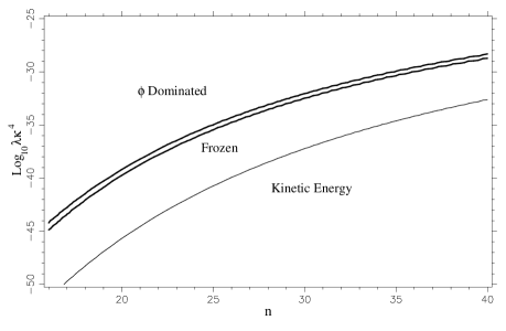
Figure 3: Regions in the parameter space where the field at the present epoch is dominated by either its kinetic or potential energy. For each point in the $(\lambda,n)$ plane, initial conditions are chosen in the numerical calculation to correspond to the conditions at the end of successful inflation. The dependence on the coupling parameter, $M$, has been eliminated by imposing the COBE normalization constraint (3.9) and the ratio of scalar field energy density to that of ordinary matter is calculated assuming $\Omega_{\rm matter}h^{2}\approx 0.3\times 0.65^{2}$. The four–dimensional Planck mass is $m^{2}_{4}=8\pi/\kappa^{2}$.

4 Discussion

In this paper, we have considered models of inflation in the second Randall–Sundrum braneworld scenario. It was found that the consistency equation (2.15) relating the tensor and scalar perturbation spectra is independent of the brane tension to lowest–order in the slow–roll approximation. This equation is given entirely in terms of observable parameters and is also independent of the functional form of the potential driving inflation. In the event of a positive detection of a primordial gravitational wave background, confirmation of such a relationship would provide strong support for inflation. However, one could not determine from this equation alone whether inflation arose within the context of a braneworld scenario or from standard relativistic cosmology. In the latter case, next–order corrections in the slow–roll parameters lead to corrections involving the scalar spectral index and it would be interesting to determine whether similar terms arise in the braneworld model. This would involve extending the analyses of Refs. [18] and [25] along the lines discussed in Ref. [34].

Furthermore, we have found that for the inverse power law potential, the scalar field can successfully drive braneworld inflation and, for appropriate choices of parameters, can act as the quintessence field at the present epoch. The spectral indices of the scalar and tensor perturbations are only weakly dependent on the power of the potential, $n$. A detectable tilt towards larger wavelengths is predicted for the scalar perturbations and the gravitational wave amplitude is within the range of sensitivity anticipated for the Planck satellite. In view of this, it is expected that models of this type should produce a CMB power spectrum where the first acoustic peak is relatively low. Although a detailed analysis of the anisotropies produced is beyond the scope of the present work, such an investigation may provide further observational tests of these models in light of the recent measurements of the first acoustic peak [1].

Acknowledgments GH is supported by the Particle Physics and Astronomy Research Council (PPARC). JEL is supported by the Royal Society. We thank A. Liddle for a helpful discussion.

References

- [1] P. de Bernardis et al., Nat. 404, 955 (2000); A. E. Lange et al., Phys. Rev. D63, 042001 (2001); A. Balbi et al., Ap. J. 545, L1 (2000).
- [2] D. H. Lyth and A. Riotto, Phys. Rep. 314, 1 (1999); M. Kamionkowski and A. Kosowsky, Ann. Rev. Nucl. Part. Sci. 49, 77 (1999); A. R. Liddle and D. H. Lyth, Cosmological Inflation and Large Scale Structure (Cambridge University Press, Cambridge, 2000).
- [3] J. E. Lidsey, A. R. Liddle, E. W. Kolb, E. W. Copeland, T. Barreiro, and M. Abney, Rev. Mod. Phys. 69, 373 (1997).
- [4] L. H. Ford, Phys. Rev. D35, 2955 (1987); L. P. Grishchuk and Y. V. Sidorov, Phys. Rev. D42, 3413 (1990).
- [5] B. Spokoiny, Phys. Lett. B315, 40 (1993); M. Joyce and T. Prokopec, Phys. Rev. D57, 6022 (1998).
- [6] P. Ferreira and M. Joyce, Phys. Rev. Lett. 79, 4740 (1997); Phys. Rev. D58, 023503 (1998).
- [7] P. J. E. Peebles and A. Vilenkin, Phys. Rev. D59, 063505 (1999); G. Felder, L. Kofman, and A. Linde, Phys. Rev. D60, 103505 (1999).
- [8] R. R. Caldwell, R. Dave, and P. J. Steinhardt, Phys. Rev. Lett. 80, 1582 (1998); L. Wang, R. R. Caldwell, J. P. Ostriker, and P. J. Steinhardt, Ap. J. 530, 17 (2000).
- [9] A. G. Riess, et al., Ap. J. 116, 1009 (1998); S. Perlmutter, et al., Ap. J. 517, 565 (1999).
- [10] K. Akama, hep-th/0001113; V. A. Rubakov and M. E. Shaposhnikov, Phys. Lett. B159, 22 (1985); N. Arkani–Hamed, S. Dimopoulos, and G. Dvali, Phys. Lett. B429, 263 (1998); I. Antoniadis, N. Arkani–Hamed, S. Dimopoulos, and G. Dvali, Phys. Lett. B436, 257 (1998); M. Gogberashvili, Europhys. Lett. 49, 396 (2000); L. Randall and R. Sundrum, Phys. Rev. Lett. 83, 3370 (1999).
- [11] L. Randall and R. Sundrum, Phys. Rev. Lett. 83, 4690 (1999).
- [12] P. Binetruy, C. Deffayet, U. Ellwanger, and D. Langlois, Phys. Lett. B477, 285 (2000).
- [13] P. Binetruy, C. Deffayet, and D. Langlois, Nucl. Phys. B565, 269 (2000); E. E. Flanagan, S. H. Tye, and I. Wasserman, Phys. Rev. D62, 044039 (2000); P. Kraus, JHEP 9912, 011 (1999); S. S. Gubser, hep-th/9912001.
- [14] T. Shiromizu, K. Maeda, and M. Sasaki, Phys. Rev. D62, 024012 (2000).
- [15] S. Mukohyama, Phys. Lett. B473, 241 (2000); D. Ida, JHEP 0009, 014 (2000).
- [16] C. Csaki, M. Graesser, C. Kolda, and J. Terning, Phys. Lett. B462, 34 (1999); J. M. Cline, C. Grojean, and G. Servant, Phys. Rev. Lett. 83, 4245 (1999).
- [17] N. Kaloper, Phys. Rev. D60, 123506 (1999); T. Nehei, Phys. Lett. B465, 81 (1999); A. Kehagias and E. Kiritsis, JHEP 9911, 022 (1999).
- [18] R. Maartens, D. Wands, B. Bassett, and I. Heard, Phys. Rev. D62, 041301 (2000).
- [19] R. M. Hawkins and J. E. Lidsey, Phys. Rev. D63, 041301 (2001).
- [20] E. J. Copeland, A. R. Liddle, and J. E. Lidsey, astro-ph/0006421.
- [21] R. Maartens, gr-qc/0101059.
- [22] G. G. Huey and R. Tavakol, In preparation (2001).
- [23] C. Wetterich, Nucl. Phys. B302, 668 (1988); E. J. Copeland, A. R. Liddle, and D. Wands, Phys. Rev. D57, 4686 (1998).
- [24] S. Sarkar, Rep. Prog. Phys. 59, 1493 (1996).
- [25] D. Langlois, R. Maartens, and D. Wands, Phys. Lett. B489, 259 (2000).
- [26] E. F. Bunn, A. R. Liddle, and M. White, Phys. Rev. D54, 5917 (1996); E. F. Bunn and M. White, Ap. J. 480, 6 (1997).
- [27] J. D. Barrow, Phys. Lett. B235, 40 (1990).
- [28] J. D. Barrow and A. R. Liddle, Phys. Rev. D47, 5219 (1993).
- [29] P. Binetruy, Phys. Rev. D60, 063502 (1999); P. Brax and J. Martin, Phys. Rev. D61, 103502 (2000).
- [30] P. J. E. Peebles and B. Ratra, Ap. J. 325, L17 (1988); B. Ratra and P. J. E. Peebles, Phys. Rev. D37, 3406 (1988); B. Ratra, Phys. Rev. D45, 1913 (1992).
- [31] A. Balbi, C. Baccigalupi, S. Matarrese, F. Perrotta, and N. Vittorio, Ap. J. 547, L89 (2001).
- [32] K. Maeda, astro-ph/0012313.
- [33] I. Zlatev, L. Wang, and P. J. Steinhardt, Phys. Rev. Lett. 82, 896 (1999); P. J. Steinhardt, L. Wang, and I. Zlatev, Phys. Rev. D59, 123504 (1999).
- [34] E. D. Stewart and D. H. Lyth, Phys. Lett. B302, 171 (1993).