Restoring the full velocity field in the gaseous disk of the spiral galaxy NGC 157.

This paper is the first in a series of articles devoted to the construction and analysis of three-component vector velocity fields in the gaseous disks of spiral galaxies, and to the discovery of giant anticyclones near corotation which were predicted earlier. We analyse the line-of-sight velocity field of ionized gas in the spiral galaxy NGC 157 which has been obtained in the H$\alpha$ emission line at the 6m telescope of SAO RAS. The field contains more than 11,000 velocity estimates. The existence of systematic deviations of the observed gas velocities from pure circular motion is shown. A detailed investigation of these deviations is undertaken by applying a recently formulated method based on Fourier analysis of the azimuthal distributions of the line-of-sight velocities at different distances from the galactic center. To restore the three-component vector velocity field from the observed line-of-sight velocity field, two assumptions were made:  1) the perturbed surface density and residual velocity components can be approximated to the formulae $C_{i}\,\cos(2\varphi+F_{i})$, where $C_{i}$ and $F_{i}$ are respectively the amplitude and the phase;  2) the perturbed surface density and residual velocity components satisfy the Euler equations. The correctness of both assumptions is proven on the basis of the observational data. As a result of the analysis, all the main parameters of the wave spiral pattern are determined: the corotation radius, the amplitudes and phases of the gas velocity perturbations at different radii, as well as the velocity of circular rotation of the disk corrected for the influence of the velocity perturbations connected with the spiral arms. Finally, a restoration of the vector velocity field in the gaseous disk of NGC 157 is performed. At a high confidence level, the presence of the two giant anticyclones in the reference frame rotating with the spiral pattern is shown; their sizes and the localization of their centers are consistent with the results of the analytic theory and of numerical simulations. Besides the anticyclones, the existence of cyclones in any residual velocity field is predicted. In the reference frame of the spiral pattern, detection of such cyclones is possible in the galaxies with a radial gradient of azimuthal residual velocity steeper than that of the rotation velocity.

1 Introduction

The present work is devoted to the analysis of line-of-sight velocities of the gas in the spiral galaxy NGC 157. We attempt to evaluate all three vector components of the perturbed gas velocity in the spiral density wave to find the angular velocity of the spiral pattern and the resonance locations, to obtain the rotation curve corrected for non-circular motions connected with the wave structures, and also to demonstrate the existence of a vortex structure.

Evidently, any method of restoration of the three-component vector velocity field from the observed one-component line-of-sight velocity field needs some additional assumptions, and the correctness of the restoration completely depends on the adequacy of those assumptions. Here two assumptions were made: 1) the perturbed surface density and residual velocity components in the NGC 157 can be approximated to the form $C_{i}\,\cos(2\varphi+F_{i})$, where $C_{i}$ and $F_{i}$ are respectively correspondingly the amplitude and the phase; 2) the perturbed surface density and residual velocity components satisfy the Euler equations. In the paper we show that both assumptions agree with the observational data. First, the predominance of the second Fourier harmonic of the brightness over others allows to adequately present the perturbed surface density in the form $\tilde{\sigma}$ $=$ $C_{\sigma}(r,\,t)\,\cos[2\varphi-F_{\sigma}(r)]$, whereas the prevalence of the second, third and the sine component of the first Fourier harmonics in the residual velocity field means that the perturbed velocity components were chosen correctly, in a similar manner. Second, analysis of the radial dependencies of the harmonic phases gives evidence for the existence of a connection between the line-of-sight velocity disturbances of the gas and the observed spiral arms, in agreement with what follows from the Euler equations.

In Sect. 2, a description of the observations of the galaxy is given. In Sect. 3, the results of an analysis of the line-of-sight velocity field under the approximation of pure circular motion are presented; we compare these results with the earlier published observational data and discuss residual line-of-sight velocities obtained by subtracting the model velocity field from the observed one. We find that the deviations from pure circular motion demonstrate a systematic behaviour. In Sect. 4, a simple model of the line-of-sight velocities is described, which takes into account motions in the two-armed density wave. It is shown that in this case the first three Fourier harmonics dominate throughout the line-of-sight velocity field. In Sect. 5, we present the results of the harmonic analysis of the observed line-of-sight velocity field which prove that the perturbed surface density and residual velocity components satisfy the Euler equations (i.e. the proof of the wave nature of the spiral structure). After that, restoration and analysis of the vector velocity field of the gas is performed. In Sect. 6, we show that the Fourier analysis of the line-of-sight velocity field allows us to restore the velocity field in the plane of the galaxy with a high degree of confidence. In Sect. 7, the corotation position is determined directly from the observations. It is shown that the velocity field in the reference frame rotating with the spiral pattern clearly demonstrates the presence of two banana-like anticyclones, the centers of which lie near the corotation. The last Section contains the main conclusions.

2 Observations and primary data reduction

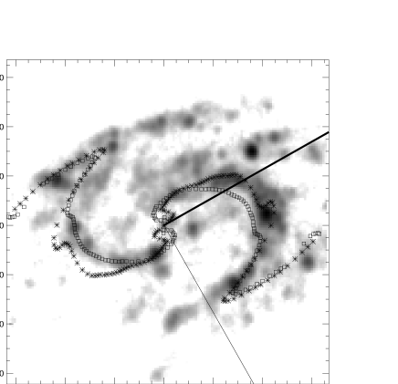
Figure 1: A monochromatic image of NGC 157 in the H$\alpha$ emission line. North is roughly to the left (PA_y $=$ $-76^{\circ}$). The phase curve of the second Fourier harmonic of the H$\alpha$ brightness map is superimposed. Asterisks show the azimuth positions of the maxima of the second harmonic at each radius. Positions of the maxima of the second Fourier harmonic of the NGC 157 $K$-band brightness map (kindly provided by S.D. Ryder) are also shown by squares.

NGC 157 (Fig. 1) is a rather bright ($B_{T}$ = 11.00) and close ($D\sim 21$ Mpc for $H_{0}$ = 75 km s^-1 Mpc^-1) isolated galaxy of SAB(rs)bc type (de Vaucouleurs et al. 1991). Its well–developed Grand–Design spiral structure is classified as Arm class 12 by Elmegreen & Elmegreen (1984). This galaxy is characterised by mildly enhanced star formation, which follows from its rather high brightness in the H$\alpha$ line and from far infrared flux densities (Ryder et al. 1998). The large angular size (the isophotal radius $D_{o}/2$ = $2.^{\prime}13$, or $\sim$ 13 kpc) and the moderate disk inclination (axis ratio $b/a$ = 0.65) make this galaxy very convenient for kinematic and photometric measurements.

The optical morphology of this galaxy is rather complex. A blue image (Lynds 1974) shows a dusty and more or less symmetrical disk with two principal spiral arms and without any hint of a bar. Nevertheless there is some evidence of a weak bar, lacking bright HII regions, in the inner part of the disk, noticeable in the red ($R$-band) image of the galaxy (Sempere & Rozas 1997). Note, however, that this bar does not reveal itself in the kinematics of Hi (Ryder et al. 1998). The spiral structure of NGC 157 is rather regular up to about $1^{\prime}$, or $\simeq$ 6.1 kpc, from the center, and, by sight, becomes flocculent or multiarmed at the periphery. As follows from the H$\alpha$ image of the galaxy, the two principal arms are not symmetrical with respect to the center (Sempere & Rozas 1997). According to Elmegreen et al. (1992) such an asymmetry may be responsible for the additional m=1 component of the spiral wave structure, driven by the two-armed spiral in the inner disk. Note also that one of the two predominant spiral arms is brighter in H$\alpha$ than the other.

Radio observations in the Hi line and at the 1.4 GHz continuum (Ryder et al. 1998) show that there is a close, though not strict correspondence of radio brightness and H$\alpha$ surface brightness. In addition, NGC 157 appears to possess an extended warped Hi disk, which stretches out well beyond the optical borders. The rotation velocity of the Hi disk amounts to about half the maximal velocity of the optical disk, which enables us to conclude that the galaxy has (1) a falling rotation curve and (2) an extended low-density halo beyond $r\sim 8-10$ kpc . The latter contains a small fraction of the total mass (about 10%) within the isophotal radius, so its gravitational input in the region of the regular spiral structure is quite negligible.

Rather bright H$\alpha$ emission is observed not only inside the spiral arms, but also between them. This circumstance is favourable for the kinematic study of the ionized gas. The first investigation of the disk kinematics was carried out by Burbidge et al. (1961) who derived a slowly rising rotation curve from two long-slit spectra. Later Zasov and Kyazumov (1981), using long-slit spectral observations at different position angles, found a significant drop of the rotational velocity at $r\simeq$ 50^′′–55^′′ in the north-eastern part of the disk. Recent Hi observations (Ryder et al. 1998) have confirmed the reality of this peculiar motion and have given evidence that it is caused both by a real declinion of the rotation curve and by asymmetry in the line-of-sight velocity distribution along the given positional angle. The optical rotation curve of the inner part of this galaxy was also obtained by Afanasiev et al. (1988). It was found that the rotation curve slowly rises, with $V_{\rm rot}\approx$ 100 km s^-1 at $r=1-2$ kpc and reaching a flat maximum of $\sim$ 200 km s^-1 at $r\sim 5-6$ kpc.

The well-defined spiral structure in the inner angular radius of one arcminute makes NGC 157 suitable for the detailed investigation of density wave propagation in the disk. Analyzing the positions of different morphological features in this galaxy, Elmegreen et al. (1992) found that corotation takes place at about $r\sim 56\arcsec$, so that the corotation circle limits the region of regular spiral structure. Note, however, that the determination of the location of resonances by morphological tracers involves a high degree of uncertainty (see the discussion in Sempere & Rozas 1997). The alternative approach used by Sempere & Rozas (1997) is based on numerical simulations of the motions of interstellar molecular clouds in the stellar disk potential, as calculated from the $R$-band image. The resulting distribution of molecular clouds has then been compared with the observed spiral structure of the galaxy. Although the results are model dependent, the obtained pattern speed in the best fit model is $\Omega_{p}$ =40 km s^-1 kpc^-1, which corresponds to a corotation radius of 50″, close to the value claimed earlier by Elmegreen et al. (1992).

Here we use a quite different method, the most direct one, to investigate the interconnection between the spiral wave and the kinematic behaviour of the interstellar gas. Our method is based on a Fourier analysis of the observations of the line-of sight velocity field (Lyakhovich et al. 1997, referred hereafter as L97). Some preliminary results of this work were given in Fridman et al. (1997, referred hereafter as F97).

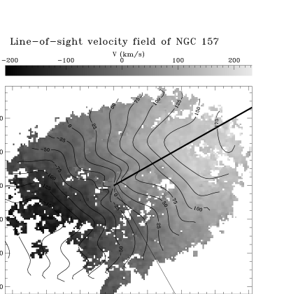
Figure 2: The line-of-sight velocity field of the gas in NGC 157 with isovelocity contours overlaid. Systematic deviations from pure circular motion, connected with the spiral arms, are clearly seen.

To obtain more detailed information about the kinematics of gaseous clouds in NGC 157, we have undertaken observations in the H$\alpha$ emission line with the scanning Fabry-Perot Interferometer (Dodonov et al. 1995) at the 6-m Telescope of the Special Astrophysical Observatory of the Russian Academy of Sciences on October 24, 1995. The Interferometer was mounted in a focal reducer ($0\aas@@fstack{\prime\prime}46$ per pixel scale) and installed at the prime focus of the telescope. To obtain 32 exposures 180 seconds each, we used the IPCS ($512\times 512$ pixels) as a detector (Afanasiev et al. 1986, 1995). Atmospheric conditions were photometric with a seeing of 2.5 arcsec. The Fabry-Perot Interferometer was tuned at the 501st order and gave a velocity sampling of 19 km s^-1. The order-separating filter with bandpass FWHM of 10 Å  ($\lambda_{c}$ $=$ 6613 Å) was used to extract the chosen etalon order. Phase calibration was made using a neon line at $\lambda=$ 6598.95 Å.

The data were reduced with the ADHOC software package, developed in Marseille Observatory (Boulesteix 1993). The resulting data cube of $256\times 256\times 32$ pixels was created with a spatial sampling of 0.92 arcsec and a velocity sampling of 19 km s^-1. The spatial resolution of 2.5 arcsec corresponds to 250-300 pc, at the distance of NGC 157 with $H_{0}$ $=$ 75 km s^-1 Mpc^-1. The line-of-sight velocity field as reduced from the data cube is shown in Fig. 2. The isovelocity contours are superimposed on this image. Even on this figure one can clearly see the systematic perturbation of the velocity field connected with the observed spiral arms. That becomes possible, in the first place, due to the continuous character of the velocity measurements, filling both the spiral arms and the interarm regions, which is what makes this particular galaxy very convenient for a detailed analysis of the velocity field.

3 Pure circular motion model and residual velocities

Systematic distortions of the line-of-sight velocity fields of a gas, induced by galactic spiral structure, are well known from observations (Lin et al. 1969; Yuan 1969; Visser 1980). The amplitude of such distortions depends on a lot of physical and geometrical parameters, particularly, on the wave amplitude, the form of the rotation curve, and the corotation position. The parameters listed above are to be determined.

The usual approach to the problem was to deal separately with the ”unperturbed” rotation curve and the residual velocity field (obtained supposedly upon subtracting the said curve from the whole picture). But the problem thus reformulated resisted all attempts to solve it in a direct way – in fact, it appears to be ill-conditioned. Indeed, to solve the problem as stated, one would have to know with high accuracy the unperturbed velocity at a given radius, which, in turn, is impossible without the knowledge of the perturbation velocities. The truth is, the problems of determining the rotation velocity and the perturbations cannot be separated, because the perturbations caused by a density wave, being non-random, affect the shape of the restored rotation curve (see below Eqs.1, 20 and discussion). The strong interdependency of both parts of the problem is where the standard methods lose their ground (L97; F97).

Figure 3: The rotation curve of NGC 157 obtained in the frame of the pure circular motion model for a set of fixed parameters of the galactic disk. Bars show errors at the level of 3 $\sigma$.

As the first step, we shall find the rotation velocity curve of the galaxy assuming the perturbations to be negligible. It helps to determine the deviations from pure rotation, to see whether their behaviour is systematic or random, and in the former case to analyse the connection of the deviations with the spiral pattern.

In the frame of this model the observed line-of-sight velocity can be written as (L97):

$$V^{\rm obs}\leavevmode\nobreak\ =\leavevmode\nobreak\ V^{\rm mod1}\leavevmode\nobreak\ +\leavevmode\nobreak\ \Psi^{\rm mod1}\,,$$

$$V^{\rm mod1}(r,\varphi)\leavevmode\nobreak\ \equiv\leavevmode\nobreak\ V^{\rm mod1}_{s}\leavevmode\nobreak\ +\leavevmode\nobreak\ V^{\rm mod1}_{\rm rot}(r)\cos\varphi\sin i\,,$$ (1)

where $\Psi^{\rm mod1}$ is the deviation of the observed velocity from the one predicted in the model of pure circular motion; $V_{s}$ is a systemic line-of-sight velocity of the galaxy; $V^{\rm mod1}_{\rm rot}$ is the model circular velocity of the gas in the plane of the galaxy which depends on the galactocentric radius $r$; $\varphi$ is the galactocentric azimuthal angle measured with respect to the major axis; $i$ is the inclination (the angle between the galactic plane and the sky plane). The usage of Eq.1 gives the real rotation velocity of the galaxy if deviations $\Psi^{\rm mod1}$ are random. Otherwise the value $V^{\rm mod1}_{\rm rot}$ will differ systematically from the true equilibrium rotation velocity $V^{eq}_{\rm rot}$ (L97, F97, see also Eqs.1, 20 and Fig. 19 below).

For the sake of definition, hereafter we identify the position $\varphi$ $=$ 0 with the major semiaxis in the receding half of the galaxy and suppose the inclination to be negative if the angular rotation momentum is directed toward the observer. In this work we have assumed that the center coordinates, the inclination, and the line-of-nodes position angle are constant parameters which do not depend on the radius. Note that variations of the disk orientation parameters along the radius (often obtained as a result of the ”splitting into rings” method of calculation of the said parameters, when each ring is considered independently), may be an artefact arising from neglecting the systematic deviations of the gas velocities from the circular ones (L97).

To determine the orientation parameters of the rotation plane of NGC 157 and its rotation curve, we have used more than 11 000 individual velocity measurements. The model parameters for the galaxy were calculated by the method of least squares, minimizing the r.m.s. deviation of the observed velocities from the model ones derived from equation (1). To estimate the rotation velocity at a radius $r$, we used the line-of-sight velocity values in the range $r-d/2$ to $r+d/2$. The value of the ring width $d$ was chosen on the basis of the following arguments. Increasing $d$ decreases the random errors, but at the same time it leads to the growth of the systematic error caused by neglecting gradients in the rotation velocity. The latter error could be estimated as $\varepsilon_{sys}$ $\approx$ $V_{\rm rot}^{\prime\prime}\,d^{2}/8$. Thus demanding the systematic error to be less than 2 km s^-1 and evaluating $V^{\prime\prime}_{\rm rot}$ $\approx$ (200 km s^-1)/(20${}^{\prime\prime})^{2}$ we come to the restriction on $d$ from above: $d$ $<$ 6^′′. On the other hand, it is meaningless to choose $d$ smaller than the seeing value (2.5^′′). For these reasons, in the analysis presented below we use $d$ $=$ 5 pixels or 4.6 arcsec. The rotation velocity was calculated at the step of one pixel (0.92 arcsec). After running through the whole range of the radial distances, we fit the rotation curve by a cubic spline.

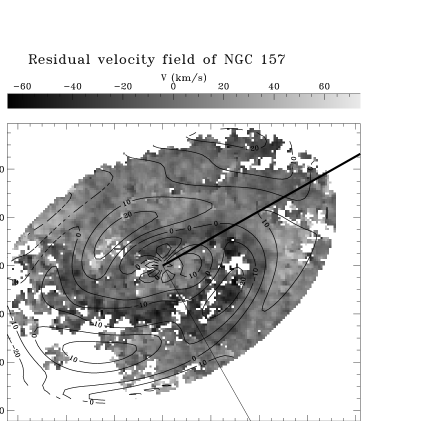
Figure 4: The field of the residual line-of-sight velocities in NGC 157 with isovelocity contours overlaid. One can see that the deviations from the pure circular motion demonstrate a systematic character.

As a result, we have obtained the following best fit parameters for NGC 157: the inclination $i=-51.5^{\circ}\pm 5^{\circ}$, the position angle of the major axis (line of nodes) PA${}_{0}=223.5^{\circ}\pm 2^{\circ}$ (we identify $PA_{0}$ with the orientation $\varphi=$ 0), and the systemic heliocentric velocity of the galaxy $V_{sys}=1667\pm 5$ km s^-1. For comparison, in the RC3 (de Vaucouleurs et al. 1991) one can find the following estimates of the systemic velocity for NGC 157: $1730\pm 27$ km s^-1 from optical data and $1668\pm 6$ km s^-1 from radio (Hi line) data. Among the above listed numerical parameters the value of $i$ was estimated less reliably. From the isophote ellipticity the inclination is known to be $i=45^{\circ}-48^{\circ}$ (Grosbøl 1985; Bottinelli et al. 1984). In the paper of Ryder et al. (1998), where the same kinematical data were used for the inner part of the galaxy and a more traditional method was applied to find the disk parameters, the inclination was found to be $i=45^{\circ}\pm 5^{\circ}$. Thus within the limits of observational errors our determination of the inclination $i$ agrees with the results of other authors.

The obtained model rotation curve $V^{\rm mod1}_{\rm rot}$ is presented in Fig. 3. The errors of the rotation velocity (3 $\sigma$) are shown by bars and are of order of 3 km s^-1 (this value represents random errors only, systematic errors caused by the neglecting of motions in the density wave could be much higher). One can see that over a wide radial range ($1-5$ kpc) $V^{\rm mod1}_{\rm rot}$ rises quite linearly with the radius $r$; the fact was pointed out earlier by Barbridge et al. (1961) and Zasov & Kyazumov (1981). This peculiarity distinguishes NGC 157 from the majority of the other spiral galaxies, for which such regions of monotonous rise of the rotation curves rarely extend beyond $2-3$ kpc.

4 The model taking into account motions in the spiral arms

In Fig. 4 we present a map of the gas residual velocities (the difference between the observed velocities and the model ones obtained from (1)). As one can see, the observed velocities deviate systematically from the pure circular motion. The regions of maximum deviations have a spiral shape, which proves their connection with the spiral density wave in this galaxy. It means that the assumptions underlying the model of pure circular motions are not valid and a more detailed model should be build.

To construct a model describing the velocity field of NGC 157 more appropriately, it is necessary to take into account motions in the density wave. In the general case, the equation, connecting the components of the full velocity vector in the galactocentric frame, $V_{r}(r,\varphi)$, $V_{\varphi}(r,\varphi)$, and $V_{z}(r,\varphi)$, with the observed line-of-sight velocity may be written as follows (L97; F97):

$$V^{\rm obs}(r,\,\varphi)\leavevmode\nobreak\ =\leavevmode\nobreak\ V_{s}\leavevmode\nobreak\ +\leavevmode\nobreak\ V_{\varphi}(r,\,\varphi)\,\cos\varphi\,\sin i\leavevmode\nobreak\ +\leavevmode\nobreak\$$

$$\leavevmode\nobreak\ +\leavevmode\nobreak\ V_{r}(r,\,\varphi)\,\sin\varphi\,\sin i\leavevmode\nobreak\ +\leavevmode\nobreak\ V_{z}(r,\,\varphi)\,\cos i\leavevmode\nobreak\ +\leavevmode\nobreak\ \Psi^{\rm obs}\,,$$ (2)

where $\Psi^{\rm obs}$ are errors in the observations. Values $V^{\rm obs}$, $V_{s}$, $V_{r}$, $V_{\varphi}$ and $V_{z}$ describe the velocity field at the moment of the observations. In other words, they are functions of the galactocentric radius $r$ and the azimuth $\varphi$ but do not depend on the time. In the case of pure circular motion, $V_{\varphi}(r,\,\varphi)$ $=$ $V^{\rm mod1}_{\rm rot}(r)$, $V_{r}(r,\,\varphi)$ $=$ 0, $V_{z}(r,\,\varphi)$ $=$ 0, so this formula evidently reduces to (1).

The relation (2) is the only one between the line-of-sight velocity field and the components of the vector velocity field of the gaseous disk, which can be derived without loss of generality. As a result, the direct restoration of the velocity field of the gaseous disk from the line-of-sight velocity field is impossible and some indirect methods should be applied (F97).

a)

b)

Figure 5: Averaged over the radial range 5^′′ - $75^{\prime\prime}$ the contribution (dispersion given in arbitrary units) of the individual Fourier harmonics into the deviation of the brightness distribution in different bands from the azimuthal symmetry. (a) H$\alpha$ brightness map, (b) $K$-band brightness map (kindly provided by S.D. Ryder).

Particularly, one may pose the question in the following way. Let us take into account that we study a galaxy with clear two–armed spiral structure (for the general case of an $m$–armed spiral see L97; F97). As the arms are easy to trace, one may assume that the perturbed surface density of the gaseous disk $\tilde{\sigma}$ (at the moment of observation) can be approximated by the expression

$$\tilde{\sigma}\leavevmode\nobreak\ =\leavevmode\nobreak\ C_{\sigma}(r)\leavevmode\nobreak\ \cos[2\varphi-F_{\sigma}(r)]\,,$$ (3)

where $C_{\sigma}$ and $F_{\sigma}$ are the corresponding amplitude and phase.

The validity of using (3) may be checked by Fourier analysis of the optical image of the galaxy: the approach is valid if the amplitude of the second Fourier harmonic predominates over the others and its phase curve closely correlates with the observed spiral. As one can see from Fig. 5, the second harmonic dominates. The high level of the first harmonic in the H$\alpha$ brightness map is caused by the nonsymmetrical distribution of star forming regions in the observed spiral arms. In our opinion, it does not reflect the real contribution of the first Fourier harmonic into the distribution of the perturbed surface density in the gaseous disk of the galaxy. The relatively low level of the first harmonics in the $K$-band image proves this assumption. Fig. 1 demonstrates that for NGC 157 the phase curve of the second Fourier harmonic of the H$\alpha$ brightness map is in good accordance with the observed spiral pattern as well as with the second harmonic of $K$-band image of the galaxy.

In a frame of the approach described, the perturbed velocity components may be written in a similar manner:

$$\tilde{V_{r}}(r,\,\varphi)=C_{r}(r)\,\cos[2\varphi-F_{r}(r)]\,,$$ (4)

$$\tilde{V_{\varphi}}(r,\,\varphi)=C_{\varphi}(r)\,\cos[2\varphi-F_{\varphi}(r)]\,,$$ (5)

$$\tilde{V_{z}}(r,\,\varphi)=C_{z}(r)\,\cos[2\varphi-F_{z}(r)]\,.$$ (6)

The validity of this approximation also can be checked directly from the observations. Indeed, taking into account that $V_{r}(r,\,\varphi)$ $=$ $\tilde{V_{r}}(r,\,\varphi)$, $V_{\varphi}(r,\,\varphi)$ $=$ $V^{\rm mod2}_{\rm rot}(r)$ $+$ $\tilde{V_{\varphi}}(r,\,\varphi)$, $V_{z}(r,\,\varphi)$ $=$ $\tilde{V_{z}}(r,\,\varphi)$, and substituting (4) – (6) in (2), we obtain the model representation of the line-of-sight velocity (L97, F97):

$$V^{\rm mod2}(r,\,\varphi)\leavevmode\nobreak\ =\leavevmode\nobreak\ V^{\rm mod2}_{s}\leavevmode\nobreak\ +\leavevmode\nobreak\ \sin i\,\left[\,a^{\rm mod2}_{1}(r)\,\cos\varphi\leavevmode\nobreak\ +\leavevmode\nobreak\ \right.$$

$$+\leavevmode\nobreak\ b^{\rm mod2}_{1}(r)\,\sin\varphi+a^{\rm mod2}_{2}(r)\,\cos 2\varphi+b^{\rm mod2}_{2}(r)\,\sin 2\varphi\leavevmode\nobreak\ +$$

$$\left.\leavevmode\nobreak\ \leavevmode\nobreak\ \leavevmode\nobreak\ \leavevmode\nobreak\ \leavevmode\nobreak\ \leavevmode\nobreak\ \leavevmode\nobreak\ +\leavevmode\nobreak\ a^{\rm mod2}_{3}(r)\,\cos 3\varphi\leavevmode\nobreak\ +\leavevmode\nobreak\ b^{\rm mod2}_{3}(r)\,\sin 3\varphi\,\right]\,,$$ (7)

where Fourier coefficients related to the phases and amplitudes of the velocity components are:

$$a^{\rm mod2}_{1}\leavevmode\nobreak\ =\leavevmode\nobreak\ V^{\rm mod2}_{\rm rot}(r)\leavevmode\nobreak\ +\leavevmode\nobreak\ \frac{C_{r}\sin F_{r}+C_{\varphi}\cos F_{\varphi}}{2}\,,$$ (8)

$$b^{\rm mod2}_{1}\leavevmode\nobreak\ =\leavevmode\nobreak\ -\leavevmode\nobreak\ \frac{C_{r}\cos F_{r}-C_{\varphi}\sin F_{\varphi}}{2}\,,$$ (9)

$$a^{\rm mod2}_{2}\leavevmode\nobreak\ =\leavevmode\nobreak\ C_{z}\cos F_{z}\,{\rm cot}\,i\,,$$ (10)

$$b^{\rm mod2}_{2}\leavevmode\nobreak\ =\leavevmode\nobreak\ C_{z}\sin F_{z}\,{\rm cot}\,i\,,$$ (11)

$$a^{\rm mod2}_{3}\leavevmode\nobreak\ =\leavevmode\nobreak\ -\leavevmode\nobreak\ \frac{C_{r}\sin F_{r}-C_{\varphi}\cos F_{\varphi}}{2}\,,$$ (12)

$$b^{\rm mod2}_{3}\leavevmode\nobreak\ =\leavevmode\nobreak\ \frac{C_{r}\cos F_{r}+C_{\varphi}\sin F_{\varphi}}{2}\,.$$ (13)

From the above relationships (8) - (13) we can see that the contributions of the different velocity components in the azimuthal Fourier harmonics of the observed line-of-sight velocity are distributed as follows.

1. The systemic velocity of the galaxy contributes in the zeroth harmonic of the observed line-of-sight velocity.

2. The circular rotation contributes in the coefficient of cosine of the first component of the observed line-of-sight velocity.

3. The perturbed motion in the galactic plane contributes in the first and third harmonics of the observed line-of-sight velocity.

4. The vertical motion (along the rotation axis) contributes in the second harmonic of the observed line-of-sight velocity.

Figure 6: Averaged over the radial range 5^′′ - $75^{\prime\prime}$, the contribution of the individual Fourier harmonics into dispersion in the model of pure rotation. The prevalence of the first sine, second and third harmonics is clearly seen.

Thus, if a galaxy has a pure two–armed structure, the observed line-of-sight velocity field should contain the zeroth, the first, the second and the third harmonics only. Actually, if the structure is not pure two–armed as we have in the case of NGC 157 (see Sandage & Bedke 1994), and yet the two–armed mode dominates, one can expect a dominance of these harmonics in the observed line-of-sight velocity field (F97).

Fig. 6 shows, for NGC 157, the contributions of the different Fourier harmonics to dispersion in the model of pure rotation averaged over the radius range 5^′′ - 75^′′. It is clearly seen that the deviations are mainly determined by the first (sine), second, and third harmonics. The individual contributions of any higher harmonic are relatively small.

Hence, the observations of NGC 157 within the radial range mentioned above justify the possibility to restrict the input of motions induced by the density wave to the main ($2\varphi$) component only. It allows the use of relations (8) – (13) connecting characteristics of the perturbed velocities and Fourier coefficients of line-of-sight velocity field to restore the three-dimensional velocity field of the galaxy.

The results obtained in this way will be presented in Sec. 6. But before proceeding, we should check whether, indeed, there exists a close connection between the residual velocities and the spiral arms observed in NGC 157. So, let us turn to the Fourier analysis of the line-of-sight velocity field to prove the wave nature of the spiral structure and the observed velocity deviations from pure rotation.

5 Fourier analysis of the velocity field

5.1 Fourier analysis technique

Suppose that the inclination $i$, the position angle of the kinematical major axis (the line of nodes) PA, and the coordinates of the galactic center in the sky plane $x_{0}$ and $y_{0}$ are known (say, having been determined in some independent way).

If the observed line-of-sight velocity can be approximated by a two-dimensional analytical function of galactocentric coordinates $r$ and $\varphi$, then its expansion into a harmonic series may be presented as:

$$V^{\rm obs}=V_{s}+\sin i\sum_{n=1}^{n_{max}}\left(a^{\rm obs}_{n}(r)\cos n\varphi+b^{\rm obs}_{n}(r)\sin n\varphi\right)$$ (14)

where $n_{max}$ is the number of the highest harmonic, to be chosen for each galaxy individually.

A well–known technique has been applied to find Fourier coefficients at discrete points $r=R_{l}$ by minimising the difference

$$\chi^{2}(R_{l})=\sum_{j}\left(V_{j}(r_{j},\varphi_{j})-V_{s}-\right.$$

$$\left.\leavevmode\nobreak\ -\leavevmode\nobreak\ \sum_{n=1}^{n_{max}}\left(a^{\rm obs}_{n}(R_{l})\cos n\varphi_{j}+b^{\rm obs}_{n}(R_{l})\sin n\varphi_{j}\right)\sin i\right)^{2}\,.$$ (15)

To construct r. m. s. deviations $\chi^{2}(R_{l})$ we use the observed values of $V_{j}$ with the coordinates $r_{j}$ falling in the galactocentric radius range from $R_{l}-d/2$ to $R_{l}+d/2$ with $d$ $=$ 4.6 arcsec (see discussion on the choice of $d$ in Sec.3). Finally, to find $a^{\rm obs}_{n}(r)$ and $b^{\rm obs}_{n}(r)$ in intermediate points $r$ we use the cubic spline drawn through the calculated points $a^{\rm obs}_{n}(R_{l})$ and $b^{\rm obs}_{n}(R_{l})$.

The recent investigation by Burlak et al. (2001) has shown that the method described here is very stable, and that its results are practically insensitive to the presence of ’holes’ in the velocity fields if the filling factor of points with velocity measurements for a given galactocentric ring is greater than 30%.

5.2 The large-scale line-of-sight velocity field

The square root of the average dispersion in the model of pure rotation is about 19 km s^-1, whereas the random error of a velocity measurement (in one pixel) is about 14 km s^-1. As the error ($\sigma$) of the harmonic amplitude determination is about 1.5 km s^-1, the above difference is statistically significant on the level of 99%. As mentioned above, deviation from the pure rotation is mainly determined by the first (sine), second and third harmonics.

The behaviour of the main harmonics with galactocentric radius is shown in Fig. 7. Bars correspond to 3$\,\sigma$ level. This figure demonstrates that the amplitudes of the main harmonics exceed the errors substantially, and hence, their values can be determined from the observations reliably over most of the galactic disk. The first plot shows the absolute value of the first harmonic cosine coefficient. Due to the good filling of the galactic disk by the velocity measurements, the value of $a^{\rm obs}_{1}$ is close to the value calculated with no account for the contribution of the other Fourier harmonics, that is by the reverse Fourier transformation. A typical discrepancy does not exceed 1 km s^-1, which is less than the errors of the $a^{\rm obs}_{1}$ determination. The maximum difference (of the order of 5 km s^-1) takes place near the galactic center where there are only a few measurements suitable for the Fourier analysis, and at the edge of the galaxy where ”holes” exist in the observed velocity field. It should be noted that the mentioned closeness is a direct consequence of the independence of different Fourier harmonics and bears no relation to the validity of the model of pure circular motions. According to Eq. (8), the difference between $a_{1}$ and the equlibrium rotation velocity is systematicaly nonzero and about the amplitude of motions in the density wave (i.e about 10-20 km s^-1, see Fig. 19 below).

Figure 7: Radial behaviour of the main harmonics of the line-of-sight velocity field for NGC 157. Bars show the observational errors (3$\sigma$).

Now we restrict the analysed field of the line-of-sight velocity of the galaxy only to the first, second, and third harmonics:

$$V^{red}/\sin i\leavevmode\nobreak\ =\leavevmode\nobreak\ V_{sys}/\sin i\leavevmode\nobreak\ +\leavevmode\nobreak\$$

$$\leavevmode\nobreak\ +\leavevmode\nobreak\ a_{1}^{\rm obs}(r)\cos\varphi\leavevmode\nobreak\ +\leavevmode\nobreak\ b_{1}^{\rm obs}(R)\sin\varphi\leavevmode\nobreak\ +\leavevmode\nobreak\$$

$$a_{2}^{\rm obs}(r)\cos 2\varphi\leavevmode\nobreak\ +\leavevmode\nobreak\ b_{2}^{\rm obs}(r)\sin 2\varphi\leavevmode\nobreak\ +\leavevmode\nobreak\$$

$$\leavevmode\nobreak\ +\leavevmode\nobreak\ a_{3}^{\rm obs}(r)\cos 3\varphi\leavevmode\nobreak\ +\leavevmode\nobreak\ b_{3}^{\rm obs}(r)\sin 3\varphi\,.$$ (16)

The averaged velocity dispersion in the model is about 15 km s^-1. The restriction to the first three harmonics is reasonable from the goodness-of-fit point of view (see Bevington 1975) because it enables the elimination of systematic deviations of the observed velocity field from those expected in the case of pure rotation of the gas in the plane of the disk.

Fig. 8 presents the residual velocity field for this model – the observed velocity field minus the model one, restricted to the first three Fourier harmonics according to (16). As one can see, the residual velocities demonstrate a small-scale chaotic structure. The areas of maximum deviations correlate with the intense star-formation regions seen on the H$\alpha$ image of the galaxy (Fig. 1).

Figure 8: Deviations of the observed line-of-sight velocity field from that restricted to the first three Fourier harmonics. The chaotic small-scale structure of the field is clearly seen. It is caused by random errors and by small-scale motions in the star-formation regions.

Therefore we can conclude that the first three harmonics describe the large-scale structure of the velocity field rather well, while the higher-order harmonics over the major part of the galaxy have smaller amplitudes and relate mostly to small-scale distortions in the brightest star formation regions and to random errors. Hence for further analysis of the large-scale structure of the velocity field we can restrict ourselves to the first three harmonics.

In the frame of the three–harmonic model we have reevaluated the parameters of the orientation of the galactic rotation plane ($i$ and PA₀). Our calculations show that the parameters which minimize the r. m. s. deviations of the line-of-sight velocities from (16) coincide with those found in the frame of the pure circular model within the measurement errors. This is easy to explain, remembering that the harmonic coefficients oscillate along the radius (see Fig. 7), so, being averaged, their input is close to zero.

Therefore, for a given galaxy and for a given rich statistical sample of measurements of the line-of-sight velocity, the model of pure circular motion allows to find parameters of the orientation of the disk with a good accuracy, even without taking into account the motions in the spiral arms.

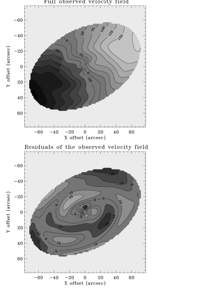
Figure 9: Large-scale component of the full (top) and residual (bottom) line-of-sight velocity fields. Only contributions of the first, second and third Fourier harmonics are included.

Fig. 9 (top) shows a model velocity field of NGC 157 in the sky plane, calculated by using the formula (16). Fig. 9 (bottom) shows a large-scale residual velocity field which represents the model velocity field upon subtraction of the first cosine harmonic. The picture of this residual velocity field is rather complex.

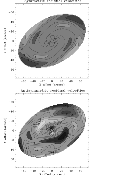
Figure 10: The symmetric (top) and antisymmetric (bottom) parts of the large-scale residual line-of-sight velocity field.

To clarify the structure of the velocity field, in Fig. 10 we present a symmetric (top) and antisymmetric (bottom) parts of the residual velocity field separately. The symmetric part contains the contribution of the second harmonic, and the antisymmetric part – contributions of the third harmonic and of the first sine harmonic.

Note that although Fig. 10 (bottom) resembles the residual velocity maps of Canzian (1993), use of Canzian’s method for the determination of the corotation radius became possible only after separating the residual velocity field into symmetric and antisymmetric components which has not been done by Canzian. As for the original field of residual velocities (Fig. 9, bottom), its shape is influenced by the second Fourier harmonic and does not contain any switching from one-armed to three-armed spiral, that is, does not allow use of Canzian’s method in principle. It is also worth mentioning that Canzian (1993) did not take the second harmonic into account at all.

5.3 Proof of the wave nature of the grand design arms

As mentioned above, the dominance of the first, second and third harmonics in the expansion of the line-of-sight velocity field of NGC 157 into Fourier series finds a natural explanation under the assumption of the wave nature of the grand design structure (see also F97).

Figure 11: Radial behaviour of the amplitude (top) and the phase (bottom) of the second Fourier harmonic of the line-of-sight velocity. Bars show the observational errors (3$\sigma$).

Let us obtain direct evidence for the latter on the base of the connection between the main Fourier harmonics of the line-of-sight velocity field and the spiral structure observed in NGC 157. To do this we consider in detail the behaviour of the second and the third Fourier harmonics. For further consideration it is convenient to define the amplitude $C_{n}$ and the phase $F_{n}$ for any harmonic by the following equations:

$$C_{n}\,\cos(F_{n})\leavevmode\nobreak\ =\leavevmode\nobreak\ a_{n}^{\rm obs}\,,$$ (17)

$$C_{n}\,\sin(F_{n})\leavevmode\nobreak\ =\leavevmode\nobreak\ b_{n}^{\rm obs}\,.$$ (18)

Fig. 11 presents radial variations of the amplitude and phase for the second harmonic of the line-of-sight velocity, following (17) and (18) for $n$ $=$ 2. The bottom plot shows the locus of the second harmonic maximum (i.e. where $\cos[2\varphi-F_{2}(R)]$ $=$ 1) on the galactic plane, which demonstrates the behaviour of the second harmonic phase. Arcs on the plot show errors of the phase determination (3 $\sigma$). As one can see, there are only a few radial positions (near $r$ $=$ $20\arcsec$ and 50″) where the amplitude of the second harmonic is comparable with the error of its measurement ($C_{2}$ $\leq$ $3\cdot\sigma_{c_{2}}$), while over most of the galaxy it is determined quite safely ($C_{2}$ $>$ $3\cdot\sigma_{c_{2}}$). The lines of the second harmonic maxima look like a two-armed trailing spiral, and they are well correlated with the galactic spiral arms observed in the emission line of H$\alpha$ inside 50″(Fig. 12). This gives strong evidence that the second harmonic of the line-of-sight velocity is related to the vertical motions in the observed spiral density wave in the region $r$ $<$ $50\arcsec$. In the outer region, the second harmonic of the line-of-sight velocity can be caused by the plane motions in $m$ $=$ 3 mode, which becomes relatively stronger in this region. A discussion of this subject is beyond the scope of the current paper.

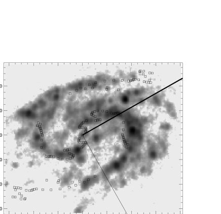
Figure 12: Superposition of the second harmonic of the line-of-sight velocity field on the H$\alpha$ image of NGC 157 (gray scale). Triangles show the azimuth positions of the maxima of the harmonic at each radius. The good correspondence of the phase curve with the observed position of the spiral arms gives strong evidence for the non-circular velocities, associated with the spiral structure.

Figure 13: Radial behaviour of the amplitude (top) and the phase (bottom) of the third Fourier harmonic of the line-of-sight velocity. Bars show the observational errors (3$\sigma$).

Fig. 13 presents the behaviour of the amplitude and phase for the third Fourier harmonic of the line-of-sight velocity field, which are defined by equations (17) and (18) for $n$ $=$ 3, as well as their errors. The bottom plot shows the locus which is determined by the equation $\cos[3\varphi-F_{3}(R)]$ $=$ 1 on the galactic plane. The amplitude of the third harmonic over most of the galaxy is determined rather reliably ($C_{3}>3\cdot\sigma_{c_{3}}$). The lines of maxima of the third harmonic also look like trailing spirals over most of the galaxy, excluding a small area at the periphery ($r$ $>$ $60\arcsec$), where they have the form of the leading spirals.

Though the spiral-like behaviour of the third harmonic is evident, a direct comparison of its pattern with the observed spiral arms of the galaxy is impossible because of the unequal number of arms. Nevertheless, it can be shown that if the observed spiral structure is a tightly wound density wave, there must exist a connection between the phase of the third Fourier harmonic of the line-of-sight velocity field and the phase of the perturbed surface density (L97; see also the Appendix below):

$$F_{3}\leavevmode\nobreak\ \approx\leavevmode\nobreak\ F_{\sigma}\leavevmode\nobreak\ +\leavevmode\nobreak\ \pi/2\,.$$ (19)

Within the corotation radius, this relation will be valid if $C_{\varphi}$ $>$ $C_{r}$. Under the opposite condition $C_{\varphi}$ $<$ $C_{r}$, $F_{3}$ $\approx$ $F_{\sigma}-\pi/2$ within the corotation radius.

To check the validity of relation (19), it is convenient to compare the locus of maxima of the observed surface density of gaseous galactic disk and two-armed spiral with the phase value equal to the phase of the third harmonic shifted by $\pi/2$. In Fig. 14 one can see the superposition of the maxima of the modified third harmonic of the line-of-sight velocity field on the maxima of the second Fourier harmonic of the $K$-band surface brightness map. The modified third harmonic varies as $\cos(2\varphi+\pi/2-F_{3})$, where $F_{3}(R)$ is the phase of the original third harmonic. The good correspondence of the phase curve with the observed position of the spiral arms (see also Fig. 1) proves that the observed deviations of the line-of-sight velocity field from the pure circular motion on one hand and the spiral arms seen in the brightness map of the galaxy on the other hand are two different manifestations of the same phenomenon – the spiral density wave.

Figure 14: Superposition of the modified third harmonic of the line-of-sight velocity field (triangles) on the second Fourier harmonic of the $K$-band brightness map of NGC 157 (squares). The modified third harmonic has a form of $\cos(2\varphi+\pi/2-F_{3})$, where $F_{3}$ is the phase of the original third harmonic. Points show the azimuth positions of the maxima of the relevant harmonic at each radius. A good agreement of the two phase curves gives strong evidence for the non-circular velocities, associated with the spiral structure.

It is worth noting that the transformation of the trailing spiral into the leading one at the periphery of the disk which is seen in Fig. 14 may be a real feature of the spiral pattern geometry, since this peculiarity appears both in the H$\alpha$ and $K$ images (see Fig. 1), as well as in the behaviour of the third Fourier harmonic of the line-of-sight velocity field (Fig. 14).

6 Determination of the vector velocity field in the plane of the galaxy

It was shown above that the large-scale structure of the velocity field may be well described in the frame of a model which includes the first, the second and the third azimuthal Fourier harmonics. It was also demonstrated that this result, as well as the structure of the line-of-sight velocity field, may be naturally explained if one suggests the residual velocities to be caused by the density wave dominated by a two–armed mode. These results allow the restoration of both the equilibrium rotation curve of the galaxy and the velocity components in the density wave, by equating correspondent Fourier coefficients in Eqs.(7) and (16):

$$V^{\rm mod2}_{\rm rot}\leavevmode\nobreak\ +\leavevmode\nobreak\ \frac{C_{r}\sin F_{r}+C_{\varphi}\cos F_{\varphi}}{2}\leavevmode\nobreak\ =\leavevmode\nobreak\ a_{1}^{\rm obs}\,,$$ (20)

$$-\leavevmode\nobreak\ C_{r}\cos F_{r}\leavevmode\nobreak\ +\leavevmode\nobreak\ C_{\varphi}\sin F_{\varphi}\leavevmode\nobreak\ =\leavevmode\nobreak\ 2\,b_{1}^{\rm obs}\,,$$ (21)

$$C_{z}\cos F_{z}\,{\rm cot}\,i\leavevmode\nobreak\ =\leavevmode\nobreak\ a_{2}^{\rm obs}\,,$$ (22)

$$C_{z}\sin F_{z}\,{\rm cot}\,i\leavevmode\nobreak\ =\leavevmode\nobreak\ b_{2}^{\rm obs}\,,$$ (23)

$$-\leavevmode\nobreak\ C_{r}\sin F_{r}\leavevmode\nobreak\ +\leavevmode\nobreak\ C_{\varphi}\cos F_{\varphi}\leavevmode\nobreak\ =\leavevmode\nobreak\ 2\,a_{3}^{\rm obs}\,,$$ (24)

$$C_{r}\cos F_{r}\leavevmode\nobreak\ +\leavevmode\nobreak\ C_{\varphi}\sin F_{\varphi}\leavevmode\nobreak\ =\leavevmode\nobreak\ 2\,b_{3}^{\rm obs}\,,$$ (25)

An additional difficulty still exists, since both rotation and motions in spiral arms contribute to the first cosine harmonic of the line-of-sight velocity. As a result of this interference, the system of equations is incomplete. Indeed, to determine seven unknown functions on the left–hand side of Eqs. (20) - (25) we have only six measured Fourier coefficients.

From Eqs. (20) - (25) it follows that the determination of the coefficients of the Fourier harmonics of the observed line-of-sight velocity field gives a possibility to determine the parameters $A_{z}$ $\equiv$ $C_{z}\cos F_{z}$, $B_{z}$ $\equiv$ $C_{z}\sin F_{z}$, $A_{r}$ $\equiv$ $C_{r}\cos F_{r}$, and $B_{\varphi}$ $\equiv$ $C_{\varphi}\sin F_{\varphi}$, without any additional assumptions. The first pair of these coefficients allows to restore the vertical velocity. $A_{r}$ characterises the behaviour of the perturbed radial velocity along the dynamical major axis of the galaxy, and $B_{\varphi}$ characterises the amplitude of the perturbed azimuthal velocity for the points at the minor axis. The radial dependencies of the coefficients $A_{r}(r)$ and $B_{\varphi}(r)$ are shown in Fig. 15.

Figure 15: Radial behaviour of the amplitudes of the cosine component for the radial residual velocity (top) and of the sine component for the azimuthal residual velocity (bottom).

However the full set of unknown parameters: $V^{\rm mod2}_{\rm rot}$, $C_{\varphi}$, $F_{\varphi}$, $C_{r}$, and $F_{r}$ cannot be derived unambiguously without additional conditions. To close the set of equations (20) - (25), we use two independent approaches proposed in L97 and F97.

6.1 Method I, based on the relation between the phases of the radial and azimuthal residual velocities

The first way to solve Eqs.(20 – 25) is to use the theoretical relation between the phases of the radial and tangential residual velocities in a tightly wound density wave (L97; F97):

$$F_{r}-F_{\varphi}\leavevmode\nobreak\ =\left\{\begin{array}[]{rl}\!\!\pi/2&\!\!{\rm at}\leavevmode\nobreak\ r<r_{c}\\ \!\!-\pi/2&\!\!{\rm at}\leavevmode\nobreak\ r>r_{c}\end{array}\!\!\right.=\leavevmode\nobreak\ -\leavevmode\nobreak\ {\mathrm{s}gn}(\hat{\omega})\,\pi/2\,.$$ (26)

By using this relation one can obtain from (20 – 25) (L97; F97):

$$V^{\rm mod2}_{\rm rot}\leavevmode\nobreak\ =\leavevmode\nobreak\ a^{\rm obs}_{1}\leavevmode\nobreak\ -\leavevmode\nobreak\ b^{\rm obs}_{1}\,a^{\rm obs}_{3}/b^{\rm obs}_{3}\,,\\$$ (27)

$$\begin{array}[]{l}A_{\varphi}\leavevmode\nobreak\ \equiv\leavevmode\nobreak\ C_{\varphi}\cos F_{\varphi}\leavevmode\nobreak\ =\leavevmode\nobreak\ a^{\rm obs}_{3}\,(b^{\rm obs}_{1}/b^{\rm obs}_{3}\leavevmode\nobreak\ +\leavevmode\nobreak\ 1)\,,\\ B_{r}\leavevmode\nobreak\ \equiv\leavevmode\nobreak\ C_{r}\sin F_{r}\leavevmode\nobreak\ =\leavevmode\nobreak\ a^{\rm obs}_{3}\,(b^{\rm obs}_{1}/b^{\rm obs}_{3}\leavevmode\nobreak\ -\leavevmode\nobreak\ 1)\,.\end{array}$$ (28)

The errors of determination of $b^{\rm obs}_{3}$ are the most crucial for application of the above relations. To avoid non-reliable estimates we assume the following condition for $b^{\rm obs}_{3}$ to be suitable for calculations: $|b^{\rm obs}_{3}|$ $>$ $3\cdot\sigma_{b^{\rm obs}_{3}}$, where $\sigma_{b^{\rm obs}_{3}}$ is an error of the measurements.

Figure 16: The rotation curve $V^{\rm mod2}_{\rm rot}$ (dashed line shows radial behaviour of $a_{1}^{\rm obs}$ which corresponds to the rotation velocity in the model of the pure circular motion, $V^{\rm mod1}_{\rm rot}$), the amplitudes of the radial and azimuthal residual velocities ($C_{r}$ and $C_{\varphi}$), the phase difference $F_{r}-F_{\varphi}$, and the localisation of the maxima of the residual radial and azimuthal velocities at each radius, obtained by using the relation between the phases of radial and tangential residual velocities. The errors are shown at the level of $3\sigma$.

Figure 17: Phase of the second harmonic of the perturbed surface density (assumed to be equal to the phase of the second harmonic of the K brightness map) and the value of $\cos F_{\sigma}$ used to calculate the parameters of the velocity field according to Method II.

Fig. 16 shows the rotation velocity ($V^{\rm mod2}_{\rm rot}$), the amplitudes and the phases of the radial and tangential residual velocities calculated from the above equations in the regions where $|b^{\rm obs}_{3}|$ $>$ $3\cdot\sigma_{b^{\rm obs}_{3}}$. For comparison, the rotation curve $V_{\rm rot}^{\rm mod1}$ obtained in the model of pure circular motion (it corresponds to the Fourier coefficient $a_{1}^{\rm obs}$) is also plotted, as a dashed line. One can see from this figure that the maxima of the radial and tangential residual velocities outline the shape of trailing spirals, whose pitch angle is close to that of the visible spiral arms. Within $7\arcsec<r<43\arcsec$, the phase difference between the radial and tangential velocities $F_{r}-F_{\varphi}$ is equal to $90^{\circ}$, and outside $r=43\arcsec$ $F_{r}-F_{\varphi}$ $=$ $-90^{\circ}$. Therefore, this method enables us to localize the corotation radius in the region around $r=43\arcsec$ (see Eq. 26). The mean amplitudes of the perturbed radial and tangential velocities are 20 – 30 km s^-1. The rotation velocity found here differs from the rotation velocity determined in the model of pure circular motion by amounts comparable to the velocity amplitude in the spiral arms.

6.2 Method II, based on the relation between the phases of the residual radial velocity and perturbed surface density

Another way to close the system of Eqs.(20 – 25) is to use the relation between the phases of the perturbed surface density and the radial residual velocity, in the approximation of tightly wound spirals (L97; F97):

$$F_{\sigma}-F_{r}\leavevmode\nobreak\ =\left\{\begin{array}[]{ll}\!\!\pi&\!\!{\rm at}\leavevmode\nobreak\ r<r_{c}\\ \!\!0&\!\!{\rm at}\leavevmode\nobreak\ r>r_{c}\end{array}\!\!\right.=\leavevmode\nobreak\ [1-{\mathrm{s}gn}(\hat{\omega})]\,\pi/2\,.$$ (29)

The determination of the perturbed density phase using the image of a galaxy is a separate problem. Here we assume that the locations of the maxima of the perturbed surface density at a given radius coincide with the locations of the maxima of the surface brightness related to the spiral arms. This assumption allows to determine the behaviour of the phase of the second Fourier harmonic of the perturbed surface density $F_{\sigma}$ by applying the Fourier analysis to the brightness distribution in a galaxy. The values of $F_{\sigma}$ and $\cos F_{\sigma}$ obtained in this way from the $K$-band image of NGC 157 (see Fig. 1) are shown in Fig. 17.

From (20) - (25) and (29) we have (L97; F97):

$$V^{\rm mod2}_{\rm rot}\leavevmode\nobreak\ =\leavevmode\nobreak\ a^{\rm obs}_{1}\leavevmode\nobreak\ -\leavevmode\nobreak\ a^{\rm obs}_{3}\leavevmode\nobreak\ -\leavevmode\nobreak\ (b^{\rm obs}_{3}-b^{\rm obs}_{1})\hbox{tan}F_{\sigma}\,,$$ (30)

$$A_{\varphi}\leavevmode\nobreak\ =\leavevmode\nobreak\ 2a^{\rm obs}_{3}\leavevmode\nobreak\ +\leavevmode\nobreak\ (b^{\rm obs}_{3}-b^{\rm obs}_{1})\,\hbox{tan}F_{\sigma}\,,$$ (31)

$$B_{r}\leavevmode\nobreak\ =\leavevmode\nobreak\ (b^{\rm obs}_{3}\leavevmode\nobreak\ -\leavevmode\nobreak\ b^{\rm obs}_{1})\,{\rm tan}\,F_{\sigma}\,.$$ (32)

Fig. 18 presents the radial dependence of the same parameters as in Fig. 16, but obtained by Method II for those regions where $\hbox{cos}F_{\sigma}$ can be determined most reliably, that is, where $|\hbox{cos}F_{\sigma}|$ $>$ $3\cdot\sigma_{\hbox{cos}F_{\sigma}}$ (see Fig. 17). As one can see from Fig. 18, the lines of the maxima of the radial and tangential velocities look like trailing spirals whose appearance agrees rather well with the phases obtained earlier by Method I (see Fig. 16). The change of the phase difference between the radial and tangential velocities from $F_{r}-F_{\varphi}$ $\simeq$ $90^{\circ}$ to $F_{r}-F_{\varphi}$ $\simeq$ $-90^{\circ}$ occurs in the radial range $36\arcsec<r<63\arcsec$. Therefore, the corotation radius obtained by this method is located within this range – in agreement with the estimate found above by Method I. The characteristic amplitudes of the radial and tangential velocities are of the order of 20 – 30 km s^-1, again in good agreement with the previous estimates.

Figure 18: AS Fig. 16, now obtained by using the relation between phases of the radial residual velocity and the perturbed surface density. The errors are shown at the level of $3\sigma$.

6.3 Final model of the velocity field

Figure 19: Rotation curve of NGC 157 in the best fit model (solid line) and in the model of pure rotation (dotted line with error bars $3\sigma$).

The most significant systematic error in the estimates obtained above arises from the assumption of a sharp switch of the phase relations near corotation. In reality, the area of switch cannot be too narrow. Our estimates show (L97) that the switch area size is of order of $1/k_{r}$, which for NGC 157 corresponds to 10″– 20″. Therefore, the velocity field parameters derived above have to be smoothed near corotation by using a filter with a width of about $1/k_{r}$.

Another argument in favour of the necessity of smoothing is the behaviour of the rotation curve near the corotation found by Methods I and II. Its non-monotonic features, seen in Figs. 16 and 18, directly result from the assumed sharp switch of the phases, since the radial distribution of the azimuthally-averaged stellar disk brightness, which follows the surface density distribution, is rather smooth and hence gives no reason to expect any peculiarities of the rotation curve near $r=30\arcsec-50\arcsec$.

So we claim the necessity to smooth the calculated rotation curve near the corotation. That, in turn, leads to a broadening of the switch area where the phase differences of the radial and tangential residual velocities and the perturbed surface density change.

To obtain the best model of the velocity field for the galaxy, the radial dependence of the residual velocities was varied within the range of uncertainties given by the comparison of Methods I and II. The ”best fit” model was chosen as a model which gives a smooth shape of the rotation curve, which can be expected for a smooth mass distribution in the galaxy. The rotation curve for the best fit model is shown in Fig. 19. For comparison, the rotation curve obtained in the traditional way, using a model of pure rotation, is also presented. In the latter case, the presence of wave-shaped features is seen. Similar wave-like details of rotation curves were found in many galaxies, and they can naturally be explained in the frame of the density wave theory (Lin et al. 1969; Yuan 1969).

Figure 20: The rotation curve $V^{\rm mod2}_{\rm rot}$ (dashed line shows the radial behaviour of $a_{1}^{\rm obs}$, which corresponds to the rotation velocity in the model of pure circular motion, $V^{\rm mod1}_{\rm rot}$), the amplitudes, the phase difference $F_{r}-F_{\varphi}$, and the positions of the maxima of radial and tangential residual velocities at different radii obtained in the best-fit model (see the text).

The estimation of the rotation velocity $V^{\rm mod2}_{\rm rot}$ at different radii enables us to determine unambiguously the other characteristics of the galactic velocity field from the set of equations (20 – 25). Fig. 20 shows the behaviour of the rotation curve, as well as that of the amplitudes and phases of radial and tangential velocities in the density wave, as obtained for the best-fit model.

7 Corotation radius of the spiral pattern

The principal aim of the present work is discovery of new galactic structures – giant anticyclones – near the corotation. To make these visible, knowledge of the corotation radius of the density wave is needed. Below we applied the methods proposed in L97 and F97 to determine the position of corotation from the observed line-of-sight velocity field of the ionized gas in the galaxy.

7.1 Method 1, using the relation between the phases of radial and tangential residual velocities

From Eqs. (20) - (25) and (26) the following relation can be obtained (L97; F97):

$$\frac{b_{3}^{\rm obs}\leavevmode\nobreak\ -\leavevmode\nobreak\ b_{1}^{\rm obs}}{b_{1}^{\rm obs}\leavevmode\nobreak\ +\leavevmode\nobreak\ b_{3}^{\rm obs}}\leavevmode\nobreak\ =\leavevmode\nobreak\ \frac{(b_{3}^{\rm obs})^{2}\leavevmode\nobreak\ -\leavevmode\nobreak\ (b_{1}^{\rm obs})^{2}}{(b_{1}^{\rm obs}\leavevmode\nobreak\ +\leavevmode\nobreak\ b_{3}^{\rm obs})^{2}}\leavevmode\nobreak\ =\leavevmode\nobreak\ \mp\leavevmode\nobreak\ \frac{C_{\varphi}}{C_{r}}\,.$$ (33)

Hereafter, the upper sign in plus-minus and minus plus signs corresponds to the region inside the corotation, and the lower sign – outside it. Taking into account that the amplitudes $C_{r}$ and $C_{\varphi}$ have always positive values, it follows from equation (33) that

$$\begin{array}[]{ll}|b_{3}^{\rm obs}(r)|-|b_{1}^{\rm obs}(r)|\leq 0,&\hbox{for\leavevmode\nobreak\ \leavevmode\nobreak\ }r<r_{c}\,,\\ |b_{3}^{\rm obs}(r)|-|b_{1}^{\rm obs}(r)|\geq 0,&\hbox{for\leavevmode\nobreak\ \leavevmode\nobreak\ }r>r_{c}\,.\end{array}$$ (34)

These inequalities offer a possibility to determine the location of corotation from the observational data. According to Eq.(34), corotation is located in the region where the difference of the amplitudes of the third sine and the first sine harmonics ($|b_{3}^{\rm obs}(r)|-|b_{1}^{\rm obs}(r)|$) changes its sign from minus to plus.

Fig. 21 shows the radial behaviour of $|b_{3}^{\rm obs}(r)|-|b_{1}^{\rm obs}(r)|$ in NGC 157. As one can see from the figure, this function is negative within the errors in the inner part of the galaxy and positive in the outer region, in accordance with the expectations. From these data it follows that the corotation radius is about $42\arcsec\pm 5\arcsec$.

Figure 21: Trend of $|b_{3}^{\rm obs}(r)|-|b_{1}^{\rm obs}(r)|$ with galactocentric radius $r$ in NGC 157. Under the approximation of tightly wound spirals this difference should be negative inside corotation and positive outside it. According to the data presented, the corotation radius is about $42\arcsec\pm 5\arcsec$. Error bars correspond to $3\sigma$ level. The jumps of the velocity components in the regions $r<20\arcsec$ and $r>65\arcsec$ unveil some peculiarities of the galactic structure in these regions. In the central area it may be ascribed to the presence of a bar, at the periphery these features are located where we observe a strong kink of spiral arms.

7.2 Method 2, using the relation between the phases of the radial residual velocity and the perturbed surface density.

System (20) - (25) closed by relation (29) gives (L97; F97):

$$(b_{3}^{\rm obs}\leavevmode\nobreak\ -\leavevmode\nobreak\ b_{1}^{\rm obs})\,\cos F_{\sigma}\leavevmode\nobreak\ =\leavevmode\nobreak\ \mp\leavevmode\nobreak\ C_{r}\,\cos^{2}F_{\sigma}\,,$$ (35)

from which follows bf that

$$\begin{array}[]{ll}(b_{3}^{\rm obs}(r)-b_{1}^{\rm obs}(r))\,\cos F_{\sigma}(r)\leavevmode\nobreak\ \leq\leavevmode\nobreak\ 0,&\leavevmode\nobreak\ \leavevmode\nobreak\ \hbox{for\leavevmode\nobreak\ }r<r_{c},\\ (b_{3}^{\rm obs}(r)-b_{1}^{\rm obs}(r))\,\cos F_{\sigma}(r)\leavevmode\nobreak\ \geq\leavevmode\nobreak\ 0,&\leavevmode\nobreak\ \leavevmode\nobreak\ \hbox{for\leavevmode\nobreak\ }r>r_{c}.\end{array}$$ (36)

These two inequalities allow to find the location of corotation on the base of the brightness map and the line-of-sight velocity field.

Fig. 22 shows the dependence of $(b_{3}^{\rm obs}-b_{1}^{\rm obs})\cos F_{\sigma}$ on galactocentric radius $r$. The estimation of $r_{c}$ by this method gives $42\arcsec\pm 6\arcsec$.

Figure 22: Variation of $(b_{3}^{\rm obs}-b_{1}^{\rm obs})\cos F_{\sigma}$ with galactocentric radius $r$ in NGC 157. In the WKB-approximation the difference should be negative inside corotation and positive outside it. Error bars correspond to $3\sigma$ level. These data show the corotation radius to be about $42\arcsec\pm 6\arcsec$.

It should be noted that the methods described above may possess not only random errors, but also some systematic errors caused by the violation of the approximation of tightly wound spirals. However they use observational data related to different parameters of the spiral structure, and their systematic errors must be different. So the results of the application of these methods give evidence that the radius of corotation is within 36″–48″and that the characteristic value of the systematic error introduced by the tightly wound approximation hardly exceeds 6″. For the second method described above, the error may be slightly higher because in this case an additional assumption about one-to-one correspondence between the azimuthal positions of the maxima of perturbed density and perturbed luminosity was made. Note that a slightly higher value for the corotation radius, $r=50\arcsec$, was recently obtained from the numerical simulation of NGC 157 by Sempere and Rozas (1997).

Assuming the location of the corotation radius to be within the radius range of 36″–48″, and taking the rotation curve as obtained in the best fit model, the inner Lindblad resonance (ILR) is either complitely absent in this galaxy, or located near the very galactic center, where the shape of the rotation curve is poorly determined. The outer Lindblad resonance (OLR) is located near the edge of the ionized-gas disk, in the region where the well-defined spiral arms end. Therefore, the bright spiral arms are constrained to exist inside the OLR. This result agrees with the results of the numerical simulations of the spiral pattern in NGC 157 (Sempere & Rozas 1997). On the other hand, a strong kink of the spiral arms (change from trailing to leading spirals) is located near the outer 4:1 resonance (compare Fig. 17 and Fig. 23).

Figure 23: Positions of the main resonances of the spiral structure in NGC 157 for the corotation position $r_{c}=42\arcsec$.

The estimate of the difference between the phases of the radial perturbed velocity and the azimuthal perturbed velocity in the best fit model allows to find the corotation radius more accurately by using the relation between the phases of radial and azimuthal velocity perturbations at the corotation. As was shown in L97, the phase difference between the radial and azimuthal perturbed velocities becomes zero at corotation. In our case, this corresponds to $r_{c}=42\arcsec$. This value will be used in the next section to restore the velocity field of the gas in the reference frame rotating with the spiral pattern.

It is worth noting that the corotation radius was found above by using some particular values of the disk inclination angle $i$ and the position angle of the line of nodes PA₀, which give the minimum dispersion in the model taking into account the first, second, and third harmonics of the line-of-sight velocity field. Any changes of these parameters, even within the errors of their determinations, may affect the determination of the location of corotation. So we have carried out a special analysis of the influence of the variations of inclination and position angle on the estimate of the corotation radius. We find that variations of the inclination by $\pm 5^{\circ}$ do not change (within the accuracy of 1″– 2″) the position of the corotation radius. However the value of $r_{c}$ strongly depends on the accepted $PA_{0}$. Variations of $PA_{0}$ by $\pm 2^{\circ}$ result in corotation radius variations of about $\sim 5\arcsec$. However, the qualitative picture of the restored velocity field remains the same even in this case.

8 Vortex structures

As a first step to visualising the restored velocity field of NGC 157, in Fig. 24 we show a vector field of the residual velocities of the gas in the plane of the galactic disk, calculated for the best fit model. We can see four vortices near $r_{c}$ – two cyclones and two anticyclones. This result is found for all values of parameters used for the restoration within the range of uncertainties.

Figure 24: Restored vector field of the residual velocity in gaseous disk of NGC 157. Overlaid squares for each galactocentric radius show azimuthal positions of maximum value of the second Fourier harmonics of the H$\alpha$ brightness map of the galaxy.

Figure 25: Restored velocity field of NGC 157 in the reference frame rotating with the pattern speed. Overlaid squares for each galactocentric radius show azimuthal positions of maximum value of the second Fourier harmonics of the H$\alpha$ brightness map of the galaxy.

The restored velocity field in the reference frame rotating with the pattern speed of the density wave, obtained in the best fit model, is shown in Fig. 25. The gas velocities inside the spiral arms are directed preferably along the arms: toward the center inside the corotation circle and outward outside the corotation. It is clearly seen that the velocity field of the galaxy demonstrates two anticyclones located in the corotation region between the spiral arms. Such anticyclonic vortices had been predicted on the basis of laboratory experiments on shallow water (Nezlin et al. 1986). The velocity amplitude of the vortices is about 30 km s^-1. The two cyclones seen in the residual velocity field are absent in the full velocity field in the reference frame corotating with the spiral arms. To make the cyclones visible, the radial gradient of the perturbed azimuthal velocity ($\partial\tilde{V}_{\varphi}/\partial r$) should be larger than the radial gradient of the rotation velocity (${\rm d}(V_{\rm rot}-\Omega_{c}r)/{\rm d}r$) in the same region of the disk. It is necessary to transform the anticyclonic shear, caused by the disk rotation, into a cyclonic shear. In the gaseous disk of NGC 157 this condition is not fulfilled. The cyclones, if they exist, must be confined to a small number of resolution elements in our data so their detection is very difficult. In galaxies with a stronger gradient of $\tilde{V}_{\varphi}$ cyclones can be observed.

As shown by numerical simulations (Baev et al. 1987; Baev & Fridman 1988), spirals and vortices are generated simultaneously by one and the same instability, already at the linear stage. The levels of saturation of the instability are different for different perturbed functions – the densities of gaseous and stellar disks and their velocities. The amplitudes of the velocities and stellar disk density perturbations stopped growing at a linear stage, while the amplitude of the gaseous disk density perturbation becomes nonlinear. As has been shown many times during the past 15 years, the streamlines of liquid particles in a self–consistent field of hydrodynamical and/or self-gravitational forces form cyclones and antycyclones (Nezlin et al. 1986; Baev & Fridman 1988; Afanasiev & Fridman 1993; Lyakhovich et al. 1996; F97). The field of the average velocity of the stellar disk under such conditions has not been calculated so far. In a general case, the structure of the field of the average velocity in the stellar systems differs substantially from the geometry of individual trajectories of stars. Contopoulos (1978) was the first to calculate individual trajectories of stars in an external gravitational potential of spiral arms. He showed that every star participates simultaneously in two motions: high-frequency (around the center of the ”epicycle”) and low-frequency (around the Lagrangian points L₂ and L₄).

As a consequence of the specific choice of the corotation radius (see the end of the previous Section), the phase difference between the azimuthal and radial residual velocities becomes zero at corotation, and both velocities simultaneously drop to zero at the centers of the vortices directly on the corotation circle. But, as was noted earlier, the qualitative picture of the restored velocity field does not depend on the particular choice of parameters within the range of their uncertainties. In all cases two anticyclones appear between the spiral arms, with their centers located near the corotation radius.

It should be noted that in reality the general picture of gas velocities in a galaxy includes not only the motions in the plane of a disk, but also vertical motions which contribute to the second Fourier harmonic of the line-of-sight velocity field (Eqs. 10, 11), and hence can be determined in the frame of the model described above (Eqs. 22, 23). The most convenient way to study vertical motions is to measure gas velocities in galaxies seen nearly face-on, where velocity components in the plane of the disk give a small contribution to the line-of-sight velocity. As an example, we refer to the analysis of the velocity field (both from Hi and H$\alpha$ observations) of the spiral galaxy NGC 3631, where vertical gas motions related to the spiral arms were really found (Fridman et al. 1998, 2000).

Comparison of the location of the spiral arms with that of the anticyclones shows that the centers of the anticyclones lie between the spiral arms. Thus, the self-gravitational forces in the gas dominate over the forces of hydrodynamic pressure in this galaxy (Lyakhovich et al. 1996). Therefore the origin of the spiral-vortex structure of NGC 157 must be explained in the frame of the gravitation concept of the density waves.

An analysis similar to the one undertaken in the present work is possible only for galaxies where the numerous estimates of the observed gas velocities are well distributed all over the disk and spiral density waves are present. It demonstrates a great potential concerning the investigation of Fourier components of the line-of-sight velocity azimuthal distributions when a sufficient amount of observational data is available.

9 Conclusions

• The line-of-sight velocity field obtained for the spiral galaxy NGC 157 from interferometric observations in the H$\alpha$ emission line, allowed us to obtain reliable estimates of the parameters of the disk orientation, of the coordinates of the dynamical center and of the rotation curve in the approximation of pure circular motion.

• Deviations of the observed line-of-sight velocities from pure circular motion have a systematic character and can be described by the first three harmonics of the Fourier expansion of the azimuthal distribution of velocities.

• When perturbed gas motions are taken into account, these do not substantially change the estimates of the disk inclination, the dynamical center position, and the major axis orientation.

• The good correspondence between two phase curves – that of the modified third harmonic of the line-of-sight velocity field and that of the second Fourier harmonic of the perturbed surface density of NGC 157, gives evidence for the wave nature of the spiral structure in this galaxy.

• The predominance of the first three Fourier harmonics in the line-of-sight velocity field is naturally explained by the prevalence of perturbations with mode $m$ $=$2 in the density wave. This circumstance opens the way to restore the full vector velocity field of the ionized gas.

• Two methods of vector velocity field restoration in a galaxy with a two-armed spiral are applied to the line-of-sight velocity field of NGC 157. They give qualitatively and quantitatively similar results. Typical values of perturbed velocities in the density wave are 20–30 km s^-1. The maximum amplitude of the radial velocity in the density wave is $\simeq 30$ km s^-1, that of the azimuthal velocity is $\simeq 40$ km s^-1.

• Using the approximation, that the pitch angle of the spiral pattern is small, we propose two methods to determine the position of the corotation radius. The first method is based solely on the Fourier analysis of the observed velocity field, and gives $r_{c}=42\arcsec\pm 5\arcsec$. The second method involves also the additional data on radial variations of the perturbed surface density phase. This method gives $r_{c}=42\arcsec\pm 6\arcsec$, which shows that these two independent approaches are in good agreement with each other.

• The determination of the corotation radius of the spiral pattern and the restoration of the gas vector velocity field in the galaxy have enabled us to detect anticyclonic structures, the existence of which had been earlier predicted analitically and from laboratory experiments on shallow water (Nezlin et al. 1986). For the galaxy NGC 157 we found that the anticyclone centers are located between the spiral arms; this gives evidence for the dominance of self-gravitation over hydrodynamic pressure forces near corotation (Lyakhovich et al. 1996).

Appendix A Derivation of basic relations

This Appendix contains a short derivation of the basic relations used in the Paper to close the system (20) - (25), in order to restore the vector velociy field of the gas, and to determine the corotation radius of the spiral structure. Whereas the final results were obtained earlier (L97; F97) the method of derivation presented here is new and more concise.

Following the traditional way of representating small amplitude perturbations in the disk (see e.g. Lin & Shu 1964; Fridman & Polyachenko 1984) we shall derive this relation below for the case of the tightly wound spiral approximation. The perturbed functions for a grand design spiral galaxy can be presented in the following form:

$$\sigma(r,\,\varphi,\,t)\leavevmode\nobreak\ =\leavevmode\nobreak\ \sigma_{0}(r)+\sigma_{1}(r,\,\varphi,\,t)\leavevmode\nobreak\ =\leavevmode\nobreak\$$

$$\leavevmode\nobreak\ \leavevmode\nobreak\ \leavevmode\nobreak\ \leavevmode\nobreak\ \leavevmode\nobreak\ =\leavevmode\nobreak\ \sigma_{0}(r)\leavevmode\nobreak\ +\leavevmode\nobreak\ \tilde{\sigma}\,\exp{\rm i}[\int\!\!k(r){\mathrm{d}}r+2\varphi-\omega t-F_{\sigma}]\,,$$ (A1)

$$V_{r}(r,\,\varphi,\,t)=V_{r1}(r,\,\varphi,\,t)=$$

$$\leavevmode\nobreak\ \leavevmode\nobreak\ \leavevmode\nobreak\ \leavevmode\nobreak\ \leavevmode\nobreak\ =\leavevmode\nobreak\ \tilde{V}_{r}\exp{\rm i}[\int\!\!k(r){\mathrm{d}}r+2\varphi-\omega t-F_{r}]\,,$$ (A2)

$$V_{\varphi}(r,\,\varphi,\,t)\leavevmode\nobreak\ =\leavevmode\nobreak\ V_{\varphi 0}(r)+V_{\varphi 1}(r,\,\varphi,\,t)\leavevmode\nobreak\ =\leavevmode\nobreak\$$

$$\leavevmode\nobreak\ \leavevmode\nobreak\ \leavevmode\nobreak\ \leavevmode\nobreak\ \leavevmode\nobreak\ =\leavevmode\nobreak\ V_{\varphi 0}(r)\leavevmode\nobreak\ +\leavevmode\nobreak\ \tilde{V}_{\varphi}\,\exp{\rm i}[\int\!\!k(r){\mathrm{d}}r+2\varphi-\omega t-F_{\varphi}]\,,$$ (A3)

where $k(r)$ is a local radial wave number, and

$$\int\!\!k(r){\mathrm{d}}r\leavevmode\nobreak\ \gg\leavevmode\nobreak\ 2\,.$$ (A4)

The latter inequality is equivalent to the tightly wound arms approximation, which is in agreement with the form of the arms of NGC 157.

Unlike the expressions (3) - (5), here we use the complex representation of the perturbed values and assume that the amplitudes marked by a tilde in Eqs. (A1) - (A3) slightly depend on $r$.

Substituting (A1) - (A3) into the linearized continuity equation for the surface density

$$\frac{\partial\sigma_{1}}{\partial t}+\frac{1}{r}\,\frac{\partial}{\partial r}(r\sigma_{0}V_{r1})+\frac{{}_{1}}{r}\frac{\partial}{\partial\varphi}(\sigma_{0}V_{\varphi 1}+\sigma_{1}V_{\varphi 0})=0$$ (A5)

and using (A4), we obtain

$$\hat{\omega}\tilde{\sigma}\exp(-iF_{\sigma})\leavevmode\nobreak\ =\leavevmode\nobreak\ \sigma_{0}k_{r}\tilde{V}_{r}\exp(-iF_{r})\,,$$ (A6)

where

$$\hat{\omega}\leavevmode\nobreak\ \equiv\leavevmode\nobreak\ \omega-2\Omega_{0}(r)\,.$$ (A7)

In most galaxies $\Omega_{0}$ is a decreasing function of $r$. Thus according to (A7) one obtains: $\hat{\omega}$ $<$ 0 inside corotation radius (at $r$ $<$ $r_{c}$) and $\hat{\omega}$ $>$ 0 outside corotation radius (at $r$ $>$ $r_{c}$). Then for a trailing spiral, $k_{r}$ $>$ 0, we find from (A6) the following relation between phases:

$$F_{\sigma}-F_{r}\leavevmode\nobreak\ =\left\{\begin{array}[]{ll}\!\!\pi&\!\!{\rm at}\leavevmode\nobreak\ r<r_{c}\\ \!\!0&\!\!{\rm at}\leavevmode\nobreak\ r>r_{c}\end{array}\!\!\right.=\leavevmode\nobreak\ [1-{\mathrm{s}gn}(\hat{\omega})]\,\pi/2\,.$$ (A8)

From the linearized equation of motion in the disk plane under the condition (A4) we obtain (Fridman & Khoruzhii, 1999):

$$\frac{V_{r1}}{V_{\varphi 1}}\leavevmode\nobreak\ =\leavevmode\nobreak\ \frac{\tilde{V}_{r}\,\exp(-{\rm i}F_{r})}{\tilde{V}_{\varphi}\,\exp(-{\rm i}F_{\varphi})}\leavevmode\nobreak\ =\leavevmode\nobreak\ {\rm i}\frac{2\Omega_{0}\hat{\omega}}{\kappa^{2}}\,,$$ (A9)

whence:

$$\exp[-{\rm i}(F_{r}-F_{\varphi})]\leavevmode\nobreak\ =\leavevmode\nobreak\ \frac{2\Omega_{0}|\hat{\omega}|}{\kappa^{2}}\,\frac{\tilde{V}_{\varphi}}{\tilde{V}_{r}}\,\exp[{\rm i}\,{\rm sgn}(\hat{\omega})\,\pi/2]\,.$$ (A10)

Here $\kappa$ is an epicyclic frequency, $\kappa^{2}$ $\equiv$ $2\Omega_{0}(2\Omega_{0}+r\Omega_{0}^{\prime})$. As follows from Fig. 3, $\kappa^{2}$ $>$ 0, therefore from (A10) we find

$$F_{r}-F_{\varphi}\leavevmode\nobreak\ =\left\{\begin{array}[]{rl}\!\!\pi/2&\!\!{\rm at}\leavevmode\nobreak\ r<r_{c}\\ \!\!-\pi/2&\!\!{\rm at}\leavevmode\nobreak\ r>r_{c}\end{array}\!\!\right.=\leavevmode\nobreak\ -\leavevmode\nobreak\ {\mathrm{s}gn}(\hat{\omega})\,\pi/2\,.$$ (A11)

Adding (A8) to (A11) and multiplying by -1 we arrive at the following relations:

$$F_{\varphi}-F_{\sigma}\leavevmode\nobreak\ =\left\{\begin{array}[]{ll}\!\!\pi/2&\!\!{\rm at}\leavevmode\nobreak\ r<r_{c}\\ \!\!\pi/2&\!\!{\rm at}\leavevmode\nobreak\ r>r_{c}\end{array}\!\!\right.=\leavevmode\nobreak\ \pi/2\,.$$ (A12)

On the other hand, from Eqs. (24), (25) taking into account (A11), one can derive

$${\rm tan}\,F_{\varphi}=\frac{b_{3}^{\rm obs}}{a_{3}^{\rm obs}},\leavevmode\nobreak\ \hbox{sgn}\left(\cos F_{\varphi}\right)=\hbox{sgn}\left[\frac{a_{3}^{\rm obs}}{(C_{\varphi}\mp C_{r}})\right]\,.$$ (A13)

Comparing the latter with the expressions derived from (17), (18):

$${\rm tan}\,F_{3}=\frac{b_{3}^{\rm obs}}{a_{3}^{\rm obs}},\leavevmode\nobreak\ \hbox{sgn}\left(\cos F_{3}\right)=\hbox{sgn}\left({a_{3}^{\rm obs}}\right)\,,$$ (A14)

we see that outside corotation the phase of the azimuthal perturbed velocity ($F_{\varphi}$) coincides with the phase of the third Fourier harmonic ($F_{3}$).

Inside corotation the relation between phases of the perturbed azimuthal velocity and the third Fourier harmonic of the observed line-of-sight velocity depends on the ratio of amplitudes $C_{\varphi}$ and $C_{r}$.

For a two–armed tightly wound spiral the ratio of amplitudes of azimuthal and radial residual velocities is (see Eq. (A9)):

$$\frac{C_{\varphi}}{C_{r}}\leavevmode\nobreak\ =\leavevmode\nobreak\ \frac{|\tilde{V}_{\varphi}|}{|\tilde{V}_{r}|}\leavevmode\nobreak\ =\leavevmode\nobreak\ \frac{\kappa^{2}}{2\Omega|\hat{\omega}|}\leavevmode\nobreak\ =\leavevmode\nobreak\ \frac{(2\Omega+r\Omega^{\prime})}{2|\Omega-\Omega_{ph}|}\,.$$ (A15)

Near corotation, this ratio is high because the denominator is small. The analysis of the rotation curve of NGC 157 (Fig. 3) shows that in the inner region of the disk the value $r{\rm d}\Omega/{\rm d}r$ is small, therefore

$$C_{\varphi}/C_{r}\leavevmode\nobreak\ \simeq\leavevmode\nobreak\ \Omega/|\Omega-\Omega_{ph}|\leavevmode\nobreak\ >\leavevmode\nobreak\ 1\,.$$ (A16)

Consequently, in most of the galactic disk the phase of the residual azimuthal velocity will be approximately equal to the phase of the third Fourier harmonic of the observed line-of-sight velocity:

$$F_{\varphi}\leavevmode\nobreak\ =\leavevmode\nobreak\ F_{3}\,.$$ (A17)

Combining the relations (A12) and (A17) we finally obtain the connection between the phases of the two observable values — perturbed surface density and third Fourier harmonic of the line-of-sight velocity:

$$F_{3}\leavevmode\nobreak\ \approx\leavevmode\nobreak\ F_{\sigma}\leavevmode\nobreak\ +\leavevmode\nobreak\ \pi/2\,.$$ (A18)

This relation should be valid if the grand design spiral has a wave nature.

The derived relations between the phases of the different parameters of the perturbations can be used to close (20) – (25) and determine the characteristics of the full vector velocity field of the galaxy.

The system of equations (20) – (25) can be rewritten as follows:

$$A_{z}\leavevmode\nobreak\ =\leavevmode\nobreak\ a_{2}^{\rm obs}{\rm cot}\,i,$$ (A19)

$$B_{z}\leavevmode\nobreak\ =\leavevmode\nobreak\ b_{2}^{\rm obs}{\rm cot}\,i,$$ (A20)

$$A_{r}\leavevmode\nobreak\ =\leavevmode\nobreak\ -b_{1}^{\rm obs}\leavevmode\nobreak\ +\leavevmode\nobreak\ b_{3}^{\rm obs},$$ (A21)

$$B_{\varphi}\leavevmode\nobreak\ =\leavevmode\nobreak\ b_{1}^{\rm obs}\leavevmode\nobreak\ +\leavevmode\nobreak\ b_{3}^{\rm obs},$$ (A22)

$$V^{\rm mod2}_{\rm rot}+A_{\varphi}\leavevmode\nobreak\ =\leavevmode\nobreak\ a_{1}^{\rm obs}\leavevmode\nobreak\ +\leavevmode\nobreak\ a_{3}^{\rm obs},$$ (A23)

$$V^{\rm mod2}_{\rm rot}+B_{r}\leavevmode\nobreak\ =\leavevmode\nobreak\ a_{1}^{\rm obs}\leavevmode\nobreak\ -\leavevmode\nobreak\ a_{3}^{\rm obs},$$ (A24)

where we have inserted the sine and cosine of the residual velocity components related to their amplitudes and phases:

$$A_{i}\leavevmode\nobreak\ =\leavevmode\nobreak\ C_{i}\,\cos F_{i}\,,$$ (A25)

$$B_{i}\leavevmode\nobreak\ =\leavevmode\nobreak\ C_{i}\,\sin F_{i}\,.$$ (A26)

The former parameter characterises the residual velocity variations along the dynamical major axis of the galaxy, and the latter describes variations along the minor axis.

It follows from (A19) - (A22) that by using only observational data, without any additional conditions, one can determine the vertical velocities in the galaxy together with the components $A_{r}$ and $B_{\varphi}$, which describe the amplitude of the perturbed radial velocity at the major axis of the galaxy and the amplitude of the perturbed azimuthal velocity at the minor axis, respectively. The vertical motions are described by the second harmonic and differ from $a_{2}^{\rm obs}\cos(2\varphi)+b_{2}^{\rm obs}\sin(2\varphi)$ only by a factor of $\hbox{cot}\,i$ which is approximately equal to 1.3 for NGC 157.

Two remaining equations, (A23) and (A24), contain three unknowns, $V^{\rm mod2}_{\rm rot}$, $A_{\varphi}$, and $B_{r}$, which cannot be determined without additional conditions.

The first way to solve Eqs.(A19) – (A24) is to use the relation (A11) between the phases of the radial and tangential residual velocities. By using this condition, from (A21), (A22), (A25) and (A26) we obtain

$$\pm\leavevmode\nobreak\ \frac{C_{r}}{C_{\varphi}}\leavevmode\nobreak\ =\leavevmode\nobreak\ \frac{b^{\rm obs}_{1}\leavevmode\nobreak\ -\leavevmode\nobreak\ b^{\rm obs}_{3}}{b^{\rm obs}_{1}\leavevmode\nobreak\ -\leavevmode\nobreak\ b^{\rm obs}_{3}}\,,$$ (A27)

and from (A23), (A24)

$$\pm\leavevmode\nobreak\ \frac{C_{r}}{C_{\varphi}}\leavevmode\nobreak\ =\leavevmode\nobreak\ \frac{a^{\rm obs}_{1}\leavevmode\nobreak\ -\leavevmode\nobreak\ a^{\rm obs}_{3}\leavevmode\nobreak\ -\leavevmode\nobreak\ V^{\rm mod2}_{\rm rot}}{a^{\rm obs}_{1}\leavevmode\nobreak\ +\leavevmode\nobreak\ a^{\rm obs}_{3}\leavevmode\nobreak\ -\leavevmode\nobreak\ V^{\rm mod2}_{\rm rot}}\,.$$ (A28)

The upper sign corresponds to the region inside corotation, and the lower sign – outside it.

By equalising the right hand terms of (A27) and (A28) we find at $r$ $<$ $r_{c}$, as well as at $r$ $>$ $r_{c}$:

$$V^{\rm mod2}_{\rm rot}\leavevmode\nobreak\ =\leavevmode\nobreak\ a^{\rm obs}_{1}\leavevmode\nobreak\ -\leavevmode\nobreak\ b^{\rm obs}_{1}\,a^{\rm obs}_{3}/b^{\rm obs}_{3}\,,\\$$ (A29)

and finally from (A23) and (A24) we get

$$\begin{array}[]{l}A_{\varphi}\leavevmode\nobreak\ =\leavevmode\nobreak\ a^{\rm obs}_{3}\,(b^{\rm obs}_{1}/b^{\rm obs}_{3}\leavevmode\nobreak\ +\leavevmode\nobreak\ 1)\,,\\ B_{r}\leavevmode\nobreak\ =\leavevmode\nobreak\ a^{\rm obs}_{3}\,(b^{\rm obs}_{1}/b^{\rm obs}_{3}\leavevmode\nobreak\ -\leavevmode\nobreak\ 1)\,.\end{array}$$ (A30)

Another way to close the system of Eqs.(A19) – (A24) is to use the relation (A8) between phases of the perturbed surface density and the radial residual velocity. The phase of the perturbed density can be determined on the basis of analysis of an image of a galaxy, assuming that the locations of the maxima of the perturbed surface density at a given radius coincide with the locations of the maxima of the surface brightness related to the spiral arms.

From (A21) and (A25) we have

$$C_{r}\,\cos\,F_{r}\leavevmode\nobreak\ =\leavevmode\nobreak\ b^{\rm obs}_{3}\leavevmode\nobreak\ -\leavevmode\nobreak\ b^{\rm obs}_{1}\,,$$ (A31)

and immediately the value $B_{r}$ is calculated, using its definition (A26) and the phase relation (A8):

$$B_{r}\leavevmode\nobreak\ =\leavevmode\nobreak\ C_{r}\,\sin\,F_{r}\leavevmode\nobreak\ =\leavevmode\nobreak\ (b^{\rm obs}_{3}\leavevmode\nobreak\ -\leavevmode\nobreak\ b^{\rm obs}_{1})\,{\rm tan}\,F_{\sigma}\,.$$ (A32)

Substituting (A32) into (A24), we find for both $r$ $<$ $r_{c}$ and $r$ $>$ $r_{c}$:

$$V^{\rm mod2}_{\rm rot}\leavevmode\nobreak\ =\leavevmode\nobreak\ a^{\rm obs}_{1}\leavevmode\nobreak\ -\leavevmode\nobreak\ a^{\rm obs}_{3}\leavevmode\nobreak\ -\leavevmode\nobreak\ (b^{\rm obs}_{3}-b^{\rm obs}_{1})\hbox{tan}F_{\sigma}\,,$$ (A33)

whence

$$A_{\varphi}\leavevmode\nobreak\ =\leavevmode\nobreak\ 2a^{\rm obs}_{3}\leavevmode\nobreak\ +\leavevmode\nobreak\ (b^{\rm obs}_{3}-b^{\rm obs}_{1})\,\hbox{tan}F_{\sigma}\,.$$ (A34)

In a similar way, the relations for determination of the corotation radius from the observational data can be derived.

From (A27), we have

$$\frac{b_{3}^{\rm obs}\leavevmode\nobreak\ -\leavevmode\nobreak\ b_{1}^{\rm obs}}{b_{1}^{\rm obs}\leavevmode\nobreak\ +\leavevmode\nobreak\ b_{3}^{\rm obs}}\leavevmode\nobreak\ =\leavevmode\nobreak\ \frac{(b_{3}^{\rm obs})^{2}\leavevmode\nobreak\ -\leavevmode\nobreak\ (b_{1}^{\rm obs})^{2}}{(b_{1}^{\rm obs}\leavevmode\nobreak\ +\leavevmode\nobreak\ b_{3}^{\rm obs})^{2}}\leavevmode\nobreak\ =\leavevmode\nobreak\ \mp\leavevmode\nobreak\ \frac{C_{\varphi}}{C_{r}}\,.$$ (A35)

Taking into account that the amplitudes $C_{r}$ and $C_{\varphi}$ always have positive values, equation (A35) gives

$$\begin{array}[]{ll}|b_{3}^{\rm obs}(r)|-|b_{1}^{\rm obs}(r)|\leq 0,&\hbox{for\leavevmode\nobreak\ \leavevmode\nobreak\ }r<r_{c}\,,\\ |b_{3}^{\rm obs}(r)|-|b_{1}^{\rm obs}(r)|\geq 0,&\hbox{for\leavevmode\nobreak\ \leavevmode\nobreak\ }r>r_{c}\,.\end{array}$$ (A36)

These inequalities offer a possibility to determine the location of corotation from the radial behaviour of $|b_{1}^{\rm obs}|$ and $|b_{3}^{\rm obs}|$ in the observed line-of-sight velocity field.

On the other hand, from (A31) we have

$$C_{r}\,\cos F_{r}\leavevmode\nobreak\ =\leavevmode\nobreak\ \mp\leavevmode\nobreak\ C_{r}\,\cos F_{\sigma}\leavevmode\nobreak\ =\leavevmode\nobreak\ b_{3}^{\rm obs}\leavevmode\nobreak\ -\leavevmode\nobreak\ b_{1}^{\rm obs}\,.$$ (A37)

Multiplying the last equality of Eq.(A37) by $\cos F_{\sigma}$, we find the equation

$$(b_{3}^{\rm obs}\leavevmode\nobreak\ -\leavevmode\nobreak\ b_{1}^{\rm obs})\,\cos F_{\sigma}\leavevmode\nobreak\ =\leavevmode\nobreak\ \mp\leavevmode\nobreak\ C_{r}\,\cos^{2}F_{\sigma}\,,$$ (A38)

from which follows

$$\begin{array}[]{ll}(b_{3}^{\rm obs}(r)-b_{1}^{\rm obs}(r))\,\cos F_{\sigma}(r)\leavevmode\nobreak\ \leq\leavevmode\nobreak\ 0,&\leavevmode\nobreak\ \leavevmode\nobreak\ \hbox{for\leavevmode\nobreak\ }r<r_{c},\\ (b_{3}^{\rm obs}(r)-b_{1}^{\rm obs}(r))\,\cos F_{\sigma}(r)\leavevmode\nobreak\ \geq\leavevmode\nobreak\ 0,&\leavevmode\nobreak\ \leavevmode\nobreak\ \hbox{for\leavevmode\nobreak\ }r>r_{c}.\end{array}$$ (A39)

These two inequalities allow to find the location of corotation on the basis of the surface brightness map and the line-of-sight velocity field.