The Globular Cluster System of NGC 1316 (Fornax A)

We have studied the Globular Cluster System of the merger galaxy NGC 1316 in Fornax, using CCD $BVI$ photometry. A clear bimodality is not detected from the broadband colours. However, dividing the sample into red (presumably metal-rich) and blue (metal-poor) subpopulations at $B-I=1.75$, we find that they follow strikingly different angular distributions. The red clusters show a strong correlation with the galaxy elongation, but the blue ones are circularly distributed. No systematic difference is seen in their radial profile and both are equally concentrated. We derive an astonishingly low Specific Frequency for NGC 1316 of only $S_{N}=0.9$, which confirms with a larger field a previous finding by Grillmair et al. (grillmair99 (1999)). Assuming a “normal” $S_{N}$ of $\sim 4$ for early-type galaxies, we use stellar population synthesis models to estimate in 2 Gyr the age of this galaxy, if an intermediate-age population were to explain the low $S_{N}$ we observe. This value agrees with the luminosity-weighted mean age of NGC 1316 derived by Kuntschner & Davies (kuntschner98 (1998)) and Mackie & Fabbiano (mackie98 (1998)). By fitting $t_{5}$ functions to the Globular Cluster Luminosity Function (GCLF), we derived the following turnover magnitudes: $B=24.69\pm 0.15$, $V=23.87\pm 0.20$ and $I=22.72\pm 0.14$. They confirm that NGC 1316, in spite of its outlying location, is at the same distance as the core of the Fornax cluster.

1 Introduction

The analysis of globular cluster systems (GCSs) in elliptical galaxies can have different motivations. One of them is to investigate the variety of GCS morphologies in relation to their host galaxy properties in order to gain insight into the formation of cluster systems (see Ashman & Zepf ashmanzepf97 (1997) and Harris harris00 (2000) for reviews).

On the other hand, GCSs have been successfully employed as distance indicators (Whitmore et al. whitmore95a (1995), Harris harris00 (2000)). This is particularly interesting if the host galaxy is simultaneously host for a type Ia supernova whose absolute luminosity can accordingly be determined, as has been the case for SN 1992A in NGC 1380 (Della Valle et al. dellavalle98 (1998)) and SN 1994D in NGC 4526 (Drenkhahn & Richtler georg99 (1999)).

However, it can happen that both aspects are equally interesting as with the target of the present contribution, NGC 1316.

NGC 1316 (Fornax A), the brightest galaxy in the Fornax cluster, is also one of the closest and brightest radio galaxies. Catalogued as a S0 peculiar galaxy, it hosted two supernovae of type Ia (SN 1980D and SN 1981N). The core of the Fornax cluster is quite compact, which makes it a better extragalactic distance standard than the Virgo cluster (see Richtler et al. tom99b (1999)). However, NGC 1316 is located relatively far out, $3\aas@@fstack{\circ}7$ away from the central giant elliptical NGC 1399.

The early studies of Schweizer (schweizer80 (1980) & schweizer81 (1981)) indicated that NGC 1316 is very probably a merger galaxy. Schweizer (schweizer80 (1980)) discovered the presence of several irregular loops and tidal tails, as well as an inclined disk of ionized gas rotating much faster than the stellar spheroid. The age of the merger event was estimated to about $4\cdot 10^{8}$–$2\cdot 10^{9}$ yrs.

Studies of galaxy mergers have shown (e.g. NGC 1275, Holtzmann et al. holtzman92 (1992), NGC 7252, Whitmore et al. whitmore93 (1993), NGC 4038/NGC 4039, Whitmore & Schweizer whitmore95b (1995)) that bright massive star clusters can form in large numbers during a merger event. But despite the strong evidence for a previous merger in NGC 1316, the only indication for cluster formation is that Grillmair et al. (grillmair99 (1999), hereafter Gr99), could not see a turnover in the GCLF at the expected magnitude. They interpreted this finding as an indication for an enhanced formation of many less massive clusters, perhaps in connection with the merger. However, their HST study was restricted to the innermost region of the galaxy.

In contrast to other galaxy mergers, where, presumably caused by the high star-formation rate (Larsen & Richtler soeren99 (1999), soeren00 (2000)), the specific frequency of GCs increases, Gr99 found an unusually small total number of clusters relative to the luminosity of NGC 1316 ($M_{V}\sim-22.8$, adopting a distance modulus to Fornax of $\mu=31.35$, Richtler et al. richtler00 (2000)).

There is also evidence from stellar population synthesis of integrated spectra that NGC 1316 hosts younger populations (Kuntschner & Davies kuntschner98 (1998), Kuntschner kuntschner00 (2000)) and thus the question arises, whether the surprisingly low specific frequency is caused by a high luminosity rather than by a small number of clusters. Goudfrooij et al. (goud00 (2000), hereafter Go00) obtained spectra of 27 globular clusters and reported that the 3 brightest clusters have an age of about 3 Gyr, indicating a high star-formation activity 3 Gyr ago, presumably caused by the merger event.

These findings and the hope for a good distance via the GCLF were the main motivation to do the present study of the GCS of NGC 1316 in a larger area than that of the HST study. As we will show, this galaxy resembles in many aspects the “old” merger galaxy NGC 5018, whose GCS has been investigated by Hilker & Kissler-Patig (hilker96 (1996)).

The paper is organized as follows: in Sect. 2 we discuss the observations, the reduction procedure and the selection of cluster candidates. The photometric and morphological properties of the GCS are discussed in Sect. 3. Sect. 4 contains our findings concerning the Specific Frequency. We conclude this work with a general discussion in Sect. 5.

2 Observations and Reduction

The $B$, $V$ and $I$ images were obtained at the $3.6$ m telescope at La Silla during the nights 29th and 30th of December, 1997 (dark moon), using the ESO Faint Object Spectrograph and Camera, EFOSC2. The field of view was $5\aas@@fstack{\prime}6\times 5\aas@@fstack{\prime}6$ with a scale of $0\aas@@fstack{\prime\prime}32$/pixel. During the first night, short- and long-exposures in each filter were centred on the galaxy. In the second night, a background field located about $5\arcmin$ away from the centre of NGC 1316 was observed, overlapping by $1\arcmin$ the observations of the first night. In addition, several fields containing standard stars from the Landolt catalog (Landolt landolt (1992)) were acquired in each filter, as well as some short exposures of NGC 1316. Fig. 1 shows the combined frames from both nights and Table 1 summarises the observations.

Table 1: Summary of the observations.

Date	Filter	Exposure (sec)	seeing
Dec. 29, 1997	$B$	$4\times 600$	$1\aas@@fstack{\prime\prime}1$
Dec. 29, 1997	$V$	$5\times 300$	$1\aas@@fstack{\prime\prime}0$
Dec. 29, 1997	$I$	$6\times 300$	$1\aas@@fstack{\prime\prime}0$
Dec. 30, 1997	$B$	$4\times 600$	$1\aas@@fstack{\prime\prime}3$
Dec. 30, 1997	$V$	$3\times 600$	$1\aas@@fstack{\prime\prime}3$
Dec. 30, 1997	$I$	$3\times 600$	$1\aas@@fstack{\prime\prime}2$

Table 2: General parameters of the target galaxy, from de Vaucouleurs et al. (devaucouleur91 (1991)) and Poulain (poulain88 (1988)).

name	$\alpha$ (2000)	$\delta$ (2000)	$l$	$b$	type	$m_{V}$	$B-V$	Veloc. [km/s]
NGC 1316	$03^{\mathrm{h}}22^{\mathrm{m}}41\aas@@fstack{s}6$	$-37\degr 06\arcmin 10\arcsec$	$240\aas@@fstack{\circ}16$	$-56\aas@@fstack{\circ}69$	(R’)SAB(s)0	$8.53\pm 0.08$	0.86	$1793\pm 12$

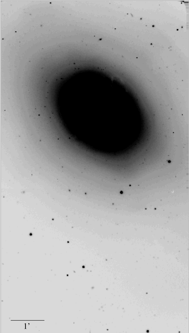
Figure 1: The entire observed field in the $B$ filter, combined from both nights. North is up, east is left.

2.1 Reduction

The frames were bias-subtracted and flat-fielded using standard IRAF procedures. Bad pixels were replaced by interpolation with neighbour pixels, using the task fixpix. The frames in each filter were then combined to remove the cosmic rays and to improve the S/N ratio. Small shifts were applied when necessary to avoid misalignment.

To perform the photometry, a relatively flat sky background must be provided. Therefore, the galaxy light needs to be subtracted. While in the case of early-type galaxies this is normally achieved by fitting elliptical isophotes (see, e.g. Jedrzejewski Jedrzejewski (1987)), NGC 1316 exhibits some substructures near its centre that can not be modeled in this way. We therefore applied a median filter, using the task median and a grid size of $35\times 35$ pixels.

After the subtraction of each combined image from its corresponding median frame, the object detection and PSF photometry was run using DAOPHOT under IRAF. The threshold level was set to $3\sigma$, and typically 2500 to 3000 objects were detected in each image. Many of these detections, particularly in the central parts of the galaxy, are spurious because of the remaining photon noise after subtraction of the galaxy model (see Sect. 2.5). Since globular clusters in the Fornax distance are not resolved, additional aperture corrections are not necessary. The object lists of the three frames were matched to remove spurious detections and to leave only objects detected in all three filters. This reduced the sample to 911 objects. We used the $(x,y)$ coordinates of this list as input for the program SExtractor (Bertin & Arnouts bertin96 (1996)), which performed the classification of point-like and galaxy-like objects by means of a “stellarity index”, calculated by a trained neural network from ellipticity and sharpness. Although SExtractor offers the possibility of performing aperture photometry, we stress that we used it only to get a better star-galaxy separation than is achievable with DAOPHOT alone.

2.2 Calibration of the photometry

A large number of standard frames were acquired in each band during the second night (the first night was not photometric). The colours of the globular clusters are well inside the range spanned by the standard stars. Aperture photometry with several annuli was performed for every standard star to construct a growth-curve (see, e.g. Stetson stetson90 (1990)). Only stars with well defined growth curves were selected. From these curves we chose an aperture radius of 30 pixels ($9\aas@@fstack{\prime\prime}6$) for the photometry of the standard stars. We then fit the instrumental magnitudes ($m_{j}$) to the equations:

$$m_{\rm b} = A_{\rm b0}+M_{\rm b}+A_{\rm b1}\cdot(B-V)+A_{\rm b2}\cdot X$$ (1)

$$m_{\rm v} = A_{\rm v0}+M_{\rm v}+A_{\rm v1}\cdot(V-I)+A_{\rm v2}\cdot X$$ (2)

$$m_{\rm i} = A_{\rm i0}+M_{\rm i}+A_{\rm i1}\cdot(V-I)+A_{\rm i2}\cdot X$$ (3)

where $A_{j0}$ and $M_{j}$ are the zeropoints and the standard apparent magnitudes, respectively. $A_{j1}$ and $A_{j2}$ are the colour and extinction coefficients. $X$ is the airmass. The fitted parameters are listed in Table 3.

Table 3: Colour and extinction coefficients for our photometry according to (1).

filter	$A_{j1}$	$A_{j2}$	rms of the fit
$B$	$-0.029\pm 0.019$	$0.220\pm 0.038$	$0.025$
$V$	$-0.049\pm 0.010$	$0.111\pm 0.017$	$0.014$
$I$	$\leavevmode\nobreak\ \leavevmode\nobreak\ \leavevmode\nobreak\ 0.023\pm 0.015$	$0.046\pm 0.029$	$0.027$

To check our photometry, we compared the magnitude and colours for NGC 1316 quoted by Poulain (poulain88 (1988)) with our values using the short-time exposures. The mean absolute differences in magnitude and colour at five aperture radii between $22\aas@@fstack{\prime\prime}9$ and $86\aas@@fstack{\prime\prime}6$ are: $\langle\Delta_{V}\rangle=0.013$, $\langle\Delta_{B-V}\rangle=0.007$ and $\langle\Delta_{V-I}\rangle=0.006$ mag, well below the rms of the fit (see Table 3). We then defined 5 local standard stars in the field of NGC 1316 to set the photometry of both nights in a consistent way.

2.3 Selection criteria

Several criteria have been applied to select cluster candidates, according to colours, magnitude, photometric errors, stellarity index and projected position around the galaxy. We assume that the clusters are similar to the Milky Way clusters. Adopting an absolute turnover magnitude (TOM) of $V=-7.60$ for the galactic clusters (Drenkhahn & Richtler georg99 (1999), Ferrarese et al. ferrarese00 (2000)) and $\mu=31.35$ (Richtler et al. richtler00 (2000)), the TOM of NGC 1316 is expected to be $V\sim 23.7$ mag, and the brightest clusters about $V\sim 20$.

Although no reddening corrections are normally applied when looking towards Fornax (Burstein & Heiles burstein82 (1982)), we cannot restrict the colours of the clusters in NGC 1316 to match exactly the galactic ones. One point is the smaller sample of galactic clusters. Besides, we must allow for significant photometric errors of faint cluster candidates. Fig. 2 shows a colour-magnitude diagram for all objects detected simultaneously in $B$, $V$ and $I$ in both nights (before the selection), together with the cut-off values adopted as criterium for this colour. As can be seen, the majority of objects have colours around $V-I=1.0$. Objects bluer than 0.5 mag are very probably foreground stars. A fraction of the data points redder than $V-I=1.6$ are background galaxies.

Figure 2: A colour-magnitude diagram for all objects detected in $B$, $V$ and $I$ in both nights before the selection criteria (911 points)

. The dashed lines indicates the selection criterium in the $V-I$ colour (see Sect. 2.3.)

We also tested in our images the robustness of the “stellarity index” computed by SExtractor. This index ranges from $0.0$ (galaxy) to $1.0$ (star) and varies for the same object by about $0.2$ when classifying under different seeing conditions, except for the brightest objects, which are clearly classified. By visual inspection of the images, we are quite confident that bright galaxies are always given indices near to zero. However, this classification becomes progressively more difficult with fainter sources.

Fig. 3 shows the “stellarity index” for the 911 objects in our sample (before the selection criteria) as a function of the magnitude. Two groups of objects having indices of $\sim 0.0$ and $\sim 1.0$ can be seen, but it is apparent that faint clusters cannot be unambiguously distinguished from background galaxies due to the uncertainty of the stellarity index in the case of faint sources. Very similar results were obtained with our “artificial stars” (see Sect. 2.5), where indices down to 0.2 were measured for faint objects that are constructed using the PSF model and, therefore, are expected to have a stellarity index of $\sim 1.0$.

Guided by our experience with artificial stars, we defined the cut-off value for the stellarity index to be 0.35. Remaining galaxies will be statistically subtracted because the same criteria are applied to the background field (see Sect. 2.4).

Figure 3: The stellarity index computed by SExtractor as function of the $V$ magnitude. The dashed lined indicates the cut value adopted in the selection criteria to reject background galaxies.

Finally, we rejected objects with photometric error larger than $0.15$ mag. To summarise, the following criteria were applied to our sample of 911 sources detected in $B$, $V$ and $I$:

• $V>19.5$

• $0.4<B-V<1.4$

• $0.3<V-I<1.8$

• stellarity index $>0.35$

• error($V$), error($B-V$), error($V-I$) $<0.15$

375 objects met this set of criteria and are our globular cluster candidates.

2.4 Background correction

After the selection, there might still be some contamination by foreground stars and background galaxies in our sample. To subtract them statistically, one needs to observe a nearby field, where no clusters are expected, and to apply the same detection and selection criteria as with the galaxy frame. However, the analysis of our background field still shows a concentration towards the galaxy centre, which means that only part of the field can be considered as background.

We used the radial profile of the GC surface densities (see Sect. 3.3) to select all objects on the flat part of the profile, i.e., where the number of globular cluster candidates per area unit exhibits no gradient. Fig. 11 (top) shows that this occurs at $r\approx 300\arcsec$, where $r$ is the distance from the optical centre. Thus, all objects with galactocentric distances larger than $300\arcsec$ and matching the above criteria, constitute our background sample.

We constructed a semi-empirical luminosity function of the background clusters with a technique described by Secker & Harris (secker93 (1993)), where a Gaussian is set over each data point, centred at the corresponding observed magnitude. The sum of all Gaussians gives a good representation of the background, without introducing an artificial undulation or loss of information due to the binning process. Fig. 4 shows the histogram of the background objects, using a bin size of $0.4$ mag, and the adopted semi-empirical function, which we use as background in the calculation of the luminosity function (see Sect. 3.4) and the specific frequency. Admittedly, the numbers are small. The dip at $V=23$ may be simply a result of bad statistics. On the other hand, as Table 6 shows, the background counts are small compared to the clusters counts. Therefore, errors of the order of the statistically expected uncertainty do not significantly influence our results and are accounted for in the uncertainties of the total counts in Table 6.

Figure 4: The semi-empirical luminosity function for the background field (dashed line). A histogram with a bin size of $0.4$ mag is over-plotted for comparison.

2.5 Completeness correction

To correct statistically for completeness, one needs to determine which fraction of objects are actually detected by the photometry routines. These ‘artificial stars experiments’ were performed using the task addstar in DAOPHOT. In one step, 100 stars were added in the science frames from $V=20$ to $V=25$ in steps of $0.1$ mag, distributed randomly to preserve the aspect of the image and not to introduce crowding as an additional parameter, but with the same coordinates in the $B$, $V$ and $I$ frames every loop. The colours of the stars were forced to be constant $B-V=0.7$ and $V-I=1.0$, close to the mean colours of the globular clusters in NGC 1316 (see Sect. 3.1). The object detection, photometry, classification and selection criteria were applied in exactly the same way as for the globular cluster candidates. To get sufficiently good statistics, we repeated the whole procedure 10 times, using different random positions in each of them and averaging the results. In all, 50000 stars were added.

However, the completeness is not only a function of the magnitude. Due to the remaining noise after galaxy subtraction, the probability of detecting an object near the centre of the galaxy is smaller than in the outer parts. We divided our sample of artificial stars into elliptical rings, in the same way as we did in deriving the radial profile (see Sect. 3.3). The results of the completeness tests are summarised in Fig. 5. It can be seen that the 50% limit goes deeper with increasing galactocentric distance.

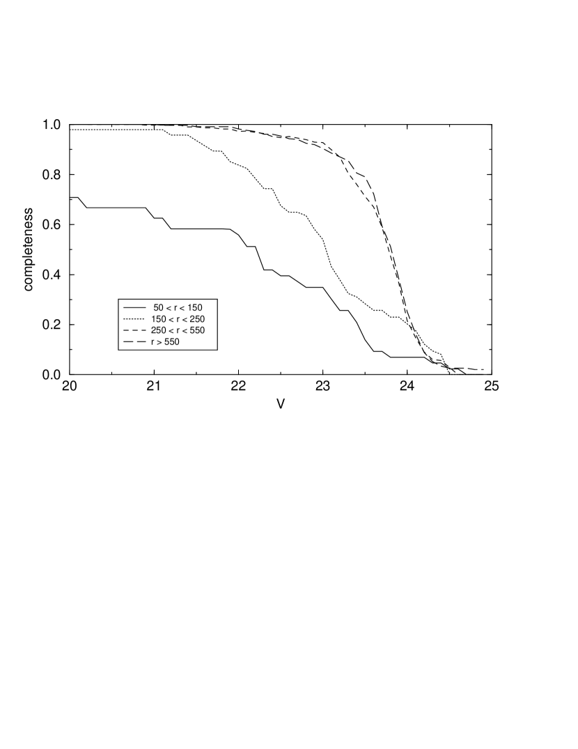
Figure 5: Completeness factors in four elliptical annuli. The probability of detection strongly decreases near the centre of NGC 1316.

3 Photometric and morphological properties

3.1 Colour distribution

In this section we discuss the colours of our GC candidates. No interstellar reddening is assumed (Burstein & Heiles burstein82 (1982)) and therefore, only internal reddening might affect the colours.

Figure 6: Colour histograms of the cluster candidates. The bin size is $0.05$ mag in each colour. A Gaussian function has been fit to the histograms (dashed line, see text). The dot-dashed line is a Gaussian with $\sigma=0.15$. The long-dashed line at $B-I=1.75$ (lower panel) was set to divide the sample in red and blue clusters.

The histograms in Fig. 6 show the colour distribution of the cluster candidates. A fit of a Gaussian function with free dispersions returned the values listed in Table 4 and is overplotted for comparison.

Table 4: Fit of a Gaussian function to the colour histograms of the GC candidates.

colour	centre	$\sigma$
$B-V$	$0.80\pm 0.02$	$0.13\pm 0.04$
$V-I$	$0.95\pm 0.01$	$0.17\pm 0.02$
$B-I$	$1.77\pm 0.02$	$0.35\pm 0.03$

As can be seen, the dispersion in the $B-V$ and $V-I$ histograms is completely explained by the photometric errors alone. This is not the case for the $B-I$ histogram, due probably to the greater metallicity sensitivity of this colour. A Gaussian with $\sigma=0.15$ mag (the maximum allowed photometric error, see Sect. 2.3) is overplotted and is clearly narrower than the colour distribution of the GCs. We use the $B-I$ broadband colour to derive a mean metallicity, as it offers the largest baseline and minimizes the effect of random photometric errors. From the calibration of Couture et al. (couture90 (1990)) for globular clusters in the Milky Way:

$$(B-I)_{0}=0.375\cdot[\@element{\mathrm{Fe}}/\@element{\mathrm{H}}]+2.147$$ (4)

the mean derived metallicity is $[\@element{\mathrm{Fe}}/\@element{\mathrm{H}}]=-1.01\pm 0.05$ dex, where the uncertainty reflects only the error in the fit of a Gaussian function to the colour histogram. The corresponding metallicity histogram is shown in Fig. 7. The clearly bimodal distribution of the galactic clusters is overplotted for comparison (dashed line). We cannot exclude that the distribution is bimodal, but then the metal-poor and the metal-rich peak are closer to each other than in the case of the galactic system.

Figure 7: Metallicity histogram of the GCS of NGC 1316, from its $B-I$ broadband colour. The galactic system (dashed line) is overplotted for comparison. The long-dashed line near $[\@element{\mathrm{Fe}}/\@element{\mathrm{H}}]=-1.0$ divides the sample in metal-rich and metal-poor clusters, using the calibration from Couture et al (couture90 (1990)) and $B-I=1.75$ (see text and Fig. 6.)

To search for colour gradients, we plotted (Fig. 8) the $B-I$ colour for the candidates, discarding the zone of the background population. Although a least-square fit to a function of the form $B-I=A\cdot 10^{m\cdot r}$gives $\Delta(B-I)/\Delta\log(r)=0.12\pm 0.07$, the data scatter too much to conclude definitely that such a gradient exists. A similar result was obtained by dividing the sample of clusters in circular rings and calculating the mean $B-I$ colour for each ring. The slope of $\Delta(B-I)/\Delta\log(r)=0.11\pm 0.07$ agrees very good with the previous fit, but it is strongly determined by the first and the last two points, where the statistic is poor. From the same plot, it is apparent that the clusters are on average $\sim 0.2$ mag bluer than the underlying galaxy light. This is a property commonly found also in normal early-type galaxies, where the blue and presumably metal-poor clusters indicate the existence of a faint metal-poor stellar (halo?) population, as the case of NGC 1380 suggests (Kissler-Patig et. al kissler97 (1997)). However, the non-existence of a colour gradient is consistent with the finding that blue and red clusters have similar surface density profiles (Sect. 3.3).

Differential reddening caused by the irregular dust structure might affect the width of the colour distribution, but apparently does not produce any colour gradient.

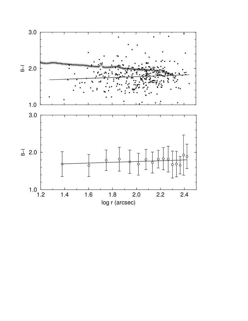
Figure 8: The $B-I$ colour gradient along the projected galactic radius. Top: the cluster candidates and a least-square fit(solid line). The crosses indicate the $B-I$ colour of the galaxy. Bottom: the mean colour in several rings, with the error bars indicating the $\sigma$ of the mean at that ring.

3.2 Angular distribution

For all objects in our sample of clusters, a transformation from cartesian $(x,y)$ coordinates to polar $(r,\theta)$ was done, with origin in the optical centre of NGC 1316. An offset of $50\degr$ in $\theta$ was applied to match the PA of the galaxy quoted by RC3. In this way, $\theta=0$ represents the direction of the semi-major axis (sma) of the galaxy, $a$, and $\theta=90\degr$ the direction of $b$, the semi-minor axis.

To analyse the angular distribution, we rejected objects inside a radius of 150 pixels (corresponding to 4.3 kpc with $\mu=31.35$), where the completeness is significantly lower (see Fig. 5) and some clusters appear over ripples and dust structures. Objects outside of 450 pixels were also rejected, as one needs equally-sized sectors to do this analysis, and $r=450$ is roughly the radius of the largest circle fully covered by our frame (see dotted line in Fig. 10). Only candidates brighter than $V=23.8$ (the 50% completeness level in the entire frame) were considered.

The data were then binned in $\theta$. Several bin sizes from $18\degr$ to $30\degr$ were tested, and Fig. 9 shows the histogram for a bin size of $22\aas@@fstack{\circ}5$, which corresponds to dividing the sample into 16 sectors. The bins were taken modulo $\pi$ for a better statistics, that is, we assume that the distribution of clusters is symmetric along the semi-mayor axis of the galaxy. Due to the substructures present in NGC 1316, and from the fact that it is a merger galaxy, one could expect some systematic differences in the azimuthal distribution of the clusters between both halves. Although this is not observed at any bin size, the small number of counts does not allow us to address this question clearly.

Figure 9: The angular distribution of globular clusters for a radius from 150 to 450 pixels ($48\arcsec$ to $144\arcsec$) down to $V=23.8$. The bin size is $22\aas@@fstack{\circ}5$ and the data were taken mod $\pi$. The histogram from $0\degr$ to $180\degr$ is repeated from $180\degr$ to $360\degr$ for a better visualisation. The dashed line indicates the best fit of a double-cosine function.

The histogram shown in Fig. 9 demonstrates the strong correlation of the globular clusters with the galaxy light. By fitting isophotes to the galaxy, we obtained ellipticities ranging from $0.27$ to $0.32$ and position angles from $49\degr$ to $53\degr$, between semi-major axes of 150 to 450 pixels (the same used with the clusters).

From the least-square fit to this histogram (with fixed period $\pi$), we derived $\mathrm{PA}=63\degr\pm 9\degr$ and an ellipticity of $0.38\pm 0.06$.

There are, however, some problems that cannot be easily resolved with our ground-based data. As indicated, the detection of cluster candidates near the centre of the galaxy is quite poor. This is, unfortunately, the most interesting region to search for young clusters which might be related to a merger event.

3.3 Radial profile

To derive the radial surface density of GCs, we divide our sample into elliptical annuli, as shown in Fig. 10. The annuli have a width of 100 pixels along the major axis ($a$) and start from $a=50$ pixels. Due to the small number of objects in the periphery of NGC 1316, rings beyond $a=900$ were given a width of 300 pixels.

Figure 10: The elliptical annuli used in the calculation of the globular cluster density and specific frequency. The open circles indicate the position of all GC candidates brighter than $V=23.8$. Objects outside the annulus defined by $r=150$ and $r=450$ pixels (dotted line) were rejected for the analysis of the angular distribution (see Sect. 3.2). Objects outside the dashed ellipse are considered as background. The scale and orientation is the same as in the Fig. 1.

The ellipticity, position angle and centre of these rings were taken from the fit of the galaxy light (see Sect. 3.2) and fixed for all annuli. In particular, the ellipticity $e$, defined as $1-(b/a)$, where $a$ and $b$ are the semi-major and semi-minor axis respectively, was set to 0.3 and the PA to $50\degr$.

We then counted the number of globular cluster candidates per unit area in each ring, down to $V=23.8$, and corrected them with the corresponding completeness function.

The results are presented in Table 5. The first column lists the mean semi-major axis of the ring. Column 2 gives the raw number of clusters down to $V=23.8$, without correction for completeness. Column 3 lists the corrected data with their errors. Column 4 lists the visible area of the rings, in $\squareforqed\arcmin$. Column 5 gives the number of candidates per unit area. Column 6, 7 and 8 are used to compute the Specific Frequency (see Sect. 4). Fig. 11 shows the radial profile of the clusters’ surface density, before and after the subtraction of the background counts.

Table 5: This table gives the result of the radial profile of the cluster candidate surface density. The first column lists the centre of each annulus (in pixels). Then follows the raw number counts down to $V=23.8$, before and after the correction for completeness. The fourth column gives the visible area of the annulus in $\squareforqed\arcmin$. Column 5 lists the mean density of GC per $\squareforqed\arcmin$. Columns 6 and 7 give the number of clusters down to the TOM in $V$, before and after the correction for completeness. The applied geometrical corrections are listed in column 8. Finally, the number of the clusters in each annulus, after doubling the counts around the TOM. Note that the corrected and total number of clusters for the innermost annulus (sma=100) are NOT derived using the completeness correction. Instead, they were estimated by extrapolating the radial profile towards the centre (see text in Sect. 4).

sma	$N^{\mathrm{raw}}_{23.8}$	$N^{\mathrm{corr}}_{23.8}$	area of ring	GC/area	$N^{\mathrm{raw}}_{\mathrm{TOM}}$	$N^{\mathrm{corr}}_{\mathrm{TOM}}$	geom. factor	$N_{\mathrm{annulus}}$
[pixels]			[$\squareforqed\arcmin$]	[$1/\squareforqed\arcmin$]
100	20	$58.6\pm 18.1$	1.251	$46.86\pm 14.47$	20	$200.2\pm 37.5$	1.	$400\pm 75$
200	53	$100.3\pm 17.9$	2.502	$40.09\pm 7.15$	53	$100.7\pm 18.0$	1.	$201\pm 36$
300	68	$104.4\pm 15.2$	3.751	$27.84\pm 4.05$	69	$109.4\pm 15.8$	1.	$219\pm 32$
400	54	$65.4\pm 10.7$	5.006	$13.06\pm 2.13$	56	$68.9\pm 11.0$	1.	$134\pm 22$
500	48	$58.2\pm 10.0$	6.234	$9.34\pm 1.60$	51	$62.0\pm 10.4$	0.997	$124\pm 21$
600	37	$42.9\pm 8.5$	6.159	$6.96\pm 1.22$	37	$44.5\pm 8.8$	0.821	$108\pm 21$
700	19	$22.4\pm 6.2$	5.145	$4.35\pm 1.21$	19	$22.8\pm 6.3$	0.588	$78\pm 21$
900	19	$23.2\pm 6.4$	9.440	$2.45\pm 0.68$	—	—	—	—
1200	11	$12.7\pm 4.6$	7.159	$1.77\pm 0.64$	—	—	—	—
1500	4	$5.3\pm 3.2$	2.880	$1.84\pm 1.11$	—	—	—	—

Figure 11: Top: the radial profile of the density of globular cluster candidates. The dashed line indicates the value adopted for the background, corresponding to $2.0$ objects$/\squareforqed\arcmin$. Bottom: the radial profile after subtraction of the background counts. The crosses represent the profile of the galaxy light, arbitrarily shifted.

A fit of a power-law $\rho(r)=A\cdot r^{\alpha}$, where $\rho$ is the surface density and $r$ the projected distance along the semi-major axis, gives $\alpha_{\mathrm{gcs}}=-2.04\pm 0.20$ and $\alpha_{\mathrm{gal}}=-2.03\pm 0.02$ for the clusters and the galaxy light, respectively. We are well aware that a King profile may be more adequate than a power function, but our purpose is to compare our result with previous work in other GCSs in Fornax, which quote only power functions.

The similarity between both slopes indicates that the GCS of NGC 1316 is not more extended than the galaxy light. Moreover, $\alpha_{\mathrm{GCS}}=-2.04$ is in good agreement with other GCS of “normal” early-type galaxies in Fornax (Kissler-Patig et al. markus97 (1997)).

We divided the system at $B-I=1.75$ mag into blue (presumably metal-poor) and red (metal-rich) clusters, and searched for systematic differences in the morphological properties between both subgroups. Again, only clusters brighter than $V=23.8$ were considered, leaving 150 blue and 166 red clusters. Our results show that both subpopulations are equally concentrated towards the centre and share the same density profile (see Fig. 12).

Figure 12: The radial profile of the GC surface density for the red (triangles) and blue population (squares). No systematic difference is seen and both are equally concentrated.

In contrast to the radial profile, red and blue clusters systematically differ in their azimuthal distribution, as shown in Fig. 13. The redder clusters show a clear correlation with the galaxy elongation, but the bluer appear to be spherically distributed, resembling a halo and bulge population. Similar results were obtained at several bin sizes.

Figure 13: The azimuthal distribution of the red (top) and blue (bottom) clusters. The bin size is $22\aas@@fstack{\circ}5$. As with Fig. 9, the data are repeated from $180\degr$ to $360\degr$ for a better visualisation. A fit of a double-sin function is overplotted for the red sample.

3.4 The luminosity function (LF)

The GCLF has been widely used as a distance indicator. The theoretical reasoning for an universality of the TOM requires an initially universal mass function of GCs in combination with a subsequent universal dynamical evolution of the individual clusters of a GCS (Okazaki & Tosa okazaki95 (1995), hereafter OT95, see e.g. Ashman & Zepf ashmanzepf97 (1997) and Harris harris00 (2000) for reviews). While the latter is plausible, as far as the average evolution is concerned, the former still lacks a theoretical explanation. Nevertheless, the empirical evidence for an universal mass function as a power law $\mathrm{d}N/\mathrm{d}M\sim M^{-1.8}$, where $\mathrm{d}N$ is the number of clusters in the mass range $M+\mathrm{d}M$, is considerable. GCSs of host galaxies of very diverse nature such as the Milky Way, ellipticals in the Virgo cluster (Harris & Pudritz harris94 (1994), McLaughlin & Pudritz mclaughlin96 (1996)) or young clusters in merging systems like NGC 4038/NGC 4039 (the Antenna, Whitmore & Schweizer whitmore95b (1995)) or NGC 7252 (Miller et al. miller97 (1997)), all show mass functions which are well described by the above power law.

However, the TOM must be a function of time, being fainter for younger cluster systems (OT95). This is due to the dynamical dissolution of clusters, which affects first the less massive ones and then progresses towards higher masses. If, for example, the red population or a part of it was formed in the merger, one would accordingly expect a fainter TOM. Therefore it is reasonable to give the LF separately for the total system, for the red, and the blue subpopulation.

The counts are given in Table 6. As stated in Sect. 2.4, only objects closer to the centre than $r=300\arcsec$ were considered possible members of the GCS of NGC 1316. Again, $r$ is measured along the major axis of an ellipse with ellipticity 0.3. The objects with $r>300\arcsec$ define the background sample. The background area is $13.72\squareforqed\arcmin$, while the area of the GCS is $38.01\squareforqed\arcmin$. We then used the results of our artificial star experiments to derive the completeness factors in four elliptical annuli: $16\arcsec<r<48\arcsec$, $48\arcsec<r<80\arcsec$, $80\arcsec<r<176\arcsec$ and $176\arcsec<r<300\arcsec$. As can be seen from Fig. 5, the completeness corrections differ at least in the three inner regions. The bin centers are given in column 1. Columns 2, 4, 6 and 8 list the counts in each region as explained above, while columns 3, 5, 7, 9 contain the corresponding completeness factors. The background counts, as defined in Sect. 2.4, are given in column 10. The total number of clusters is listed in column 11. This is the sum of the clusters in each region (corrected for completeness), minus the background level scaled to the area of counting. The uncertainties result from an error propagation, where also the error in the background was considered. A value of 0.02 has been adopted as the error in the completeness factors, which is roughly the RMS we observed between the tests.

There are two additional columns, namely the number of blue and red clusters. They were calculated in the same way and will be discussed in Sect. 5.

Bin sizes of $0.3$, $0.4$ and $0.5$ mag were tested, and the results were always in good agreement with each other. Finally, we have chosen $0.5$ mag as our bin size from the appearance of the fit histogram, and the absence of undulations which are present for the other cases.

We note, however, that our derived TOM is close to the limit of the observations, and the last bins are strongly affected by the completeness correction. Nevertheless, the similarity of the results using different bin sizes and centers, and the robustness of the fit against skipping the last bin, is encouraging.

Table 6: The counts (in bins of $0.5$ mag) used in the determination of the GCLF. Given are the $V$-magnitudes (or $B$, $I$, respectively) of the bin centers. Then follow the raw counts of the four elliptical annuli $N_{i}$ (see text) together with the corresponding completeness factors $f_{i}$. The background counts are then listed as defined in Sect. 2.4. The completeness factors of the fourth annulus have been used for the background as well. The total number of clusters is the sum of the four annuli minus the background, normalised to the same area (see text). Also given is the number of clusters for the blue and the red population separately, where the separating colour was $B-I=1.75$.

$V$	$N_{1}^{V}$	$f_{1}$	$N_{2}^{V}$	$f_{2}$	$N_{3}^{V}$	$f_{3}$	$N_{4}^{V}$	$f_{4}$	$N_{\mathrm{bkg.}}^{V}$	$N_{\mathrm{total}}^{V}$	$N_{\mathrm{blue}}^{V}$	$N_{\mathrm{red}}^{V}$
19.5	0	0.71	1	0.98	1	1.00	2	1.00	0.0	$4.0\pm 2.0$	$1.0\pm 1.0$	$3.0\pm 1.7$
20.0	1	0.71	1	0.98	3	1.00	1	1.00	0.0	$6.4\pm 2.7$	$2.4\pm 1.7$	$4.0\pm 2.0$
20.5	1	0.67	0	0.98	4	1.00	2	1.00	0.2	$6.9\pm 3.1$	$3.9\pm 2.6$	$3.0\pm 1.7$
21.0	2	0.62	6	0.98	3	1.00	3	1.00	1.0	$12.6\pm 5.0$	$1.4\pm 3.3$	$11.2\pm 3.8$
21.5	2	0.58	3	0.94	12	0.99	7	0.99	2.5	$18.8\pm 7.0$	$7.8\pm 4.6$	$11.3\pm 5.2$
22.0	2	0.56	5	0.84	14	0.97	11	0.98	4.6	$22.2\pm 8.8$	$14.4\pm 6.9$	$8.0\pm 5.4$
22.5	7	0.40	11	0.68	32	0.95	14	0.95	4.2	$69.8\pm 12.5$	$36.6\pm 9.0$	$33.3\pm 8.6$
23.0	3	0.35	18	0.54	39	0.93	14	0.90	1.7	$94.2\pm 12.9$	$44.3\pm 8.7$	$49.9\pm 9.5$
23.5	2	0.14	8	0.28	52	0.71	19	0.79	3.7	$127.2\pm 19.9$	$65.5\pm 15.6$	$61.7\pm 12.1$
24.0	0	0.07	2	0.20	32	0.22	8	0.25	3.8	$145.1\pm 38.8$	$48.8\pm 24.8$	$96.5\pm 28.1$
24.5	0	0.00	0	0.00	4	0.03	1	0.03	0.5	—	—	—

$B$	$N_{1}^{B}$	$f_{1}$	$N_{2}^{B}$	$f_{2}$	$N_{3}^{B}$	$f_{3}$	$N_{4}^{B}$	$f_{4}$	$N_{\mathrm{bkg.}}^{B}$	$N_{\mathrm{total}}^{B}$	$N_{\mathrm{blue}}^{B}$	$N_{\mathrm{red}}^{B}$
20.5	0	0.71	1	0.98	2	1.00	2	1.00	0.0	$5.0\pm 2.2$	$1.0\pm 1.0$	$4.0\pm 2.0$
21.0	2	0.67	1	0.98	3	1.00	3	1.00	0.2	$9.5\pm 3.6$	$5.4\pm 3.1$	$4.0\pm 2.0$
21.5	1	0.67	3	0.98	4	1.00	1	1.00	0.7	$7.6\pm 4.0$	$0.1\pm 2.7$	$7.6\pm 2.9$
22.0	2	0.58	4	0.96	5	1.00	4	1.00	0.7	$14.7\pm 5.0$	$7.1\pm 3.9$	$7.6\pm 3.1$
22.5	2	0.58	5	0.89	15	0.98	8	0.99	3.3	$23.2\pm 7.9$	$10.5\pm 7.0$	$12.8\pm 5.3$
23.0	5	0.42	9	0.74	24	0.96	11	0.96	4.8	$46.7\pm 11.1$	$32.0\pm 9.7$	$13.8\pm 6.5$
23.5	4	0.35	11	0.64	31	0.94	17	0.92	3.2	$70.4\pm 12.0$	$35.2\pm 8.6$	$35.3\pm 9.1$
24.0	3	0.26	14	0.32	50	0.80	15	0.85	2.3	$127.9\pm 17.8$	$57.8\pm 16.5$	$70.1\pm 13.1$
24.5	1	0.07	6	0.23	47	0.47	13	0.51	4.8	$139.8\pm 27.6$	$66.7\pm 33.2$	$73.1\pm 16.4$
25.0	0	0.05	1	0.09	15	0.06	7	0.05	2.0	$290.3\pm 159.0$	—	—
25.5	0	0.00	0	0.00	0	0.00	1	0.02	0.1	—	—	—

$I$	$N_{1}^{I}$	$f_{1}$	$N_{2}^{I}$	$f_{2}$	$N_{3}^{I}$	$f_{3}$	$N_{4}^{I}$	$f_{4}$	$N_{\mathrm{bkg.}}^{I}$	$N_{\mathrm{total}}^{I}$	$N_{\mathrm{blue}}^{I}$	$N_{\mathrm{red}}^{I}$
18.5	0	0.71	1	0.98	0	1.00	2	1.00	0.0	$3.0\pm 1.7$	$0.0\pm 0.0$	$3.0\pm 1.7$
19.0	0	0.71	1	0.98	4	1.00	1	1.00	0.0	$6.0\pm 2.5$	$1.0\pm 1.0$	$5.0\pm 2.2$
19.5	3	0.67	1	0.98	3	1.00	0	1.00	0.0	$8.5\pm 3.3$	$4.0\pm 2.3$	$4.5\pm 2.3$
20.0	0	0.63	5	0.98	3	1.00	5	1.00	0.5	$11.7\pm 4.1$	$3.2\pm 2.5$	$8.5\pm 3.3$
20.5	4	0.58	4	0.94	11	0.99	5	0.99	2.8	$19.8\pm 7.4$	$9.5\pm 4.9$	$10.3\pm 5.5$
21.0	2	0.56	6	0.84	16	0.97	10	0.98	3.8	$26.7\pm 8.5$	$9.3\pm 5.4$	$17.4\pm 6.6$
21.5	4	0.40	9	0.68	35	0.95	17	0.95	5.1	$63.1\pm 12.1$	$33.0\pm 9.0$	$30.1\pm 8.0$
22.0	5	0.35	18	0.54	37	0.93	12	0.90	1.9	$94.9\pm 13.5$	$39.0\pm 9.2$	$55.9\pm 9.8$
22.5	1	0.14	9	0.28	46	0.71	15	0.79	2.3	$115.0\pm 17.9$	$62.0\pm 13.9$	$53.4\pm 10.9$
23.0	1	0.07	0	0.20	38	0.22	15	0.25	4.3	$199.4\pm 45.4$	$130.6\pm 36.4$	$68.8\pm 24.6$
23.5	0	0.02	1	0.00	3	0.03	0	0.03	1.4	—	—	—

Fig. 14 shows the three luminosity functions in $B$, $V$, $I$. For fitting the LF we chose $t_{5}$ functions, which are of the form:

$$t_{5}(m)=\frac{8}{3\sqrt{5}\pi\sigma_{t}}\left(1+\frac{(m-m_{0})^{2}}{5\sigma_{t}^{2}}\right)^{-3}$$ (5)

Gaussians give no significantly different results, as earlier investigations have demonstrated (e.g. Della Valle et al. dellavalle98 (1998)). Since our photometry is not deep enough to fit $\sigma_{t}$ independently, we used a fixed value of $\sigma_{t}=1.1$, which is appropriate for early-type galaxies (Harris harris00 (2000) quotes $1.4$ as a typical Gaussian dispersion, while $1.29$ is the ratio between the Gaussian dispersion and the dispersion of a $t_{5}$-function).

Table 7 lists the TOMs for the three bands $B$, $V$ and $I$, additionally the TOMs for the blue and the red population in all filters. The uncertainties are the formal fit errors accounting also for the count uncertainties in the individual bins, as given in Table 6.

It is apparent that the TOMs are not convincingly reached in the full sample. Moreover, it is clear that we cannot say anything definitive about a possibly different TOM for the red and the blue population. Deeper photometry is required.

The formal distance moduli, resulting from the full sample, are $31.58\pm 0.18$ in $B$, $31.47\pm 0.22$ in $V$, and $31.19\pm 0.17$ in $I$, adopting as the absolute TOMs $M^{T}_{B}=-6.89\pm 0.10$, $M^{T}_{V}=-7.60\pm 0.08$ and $M^{T}_{I}=-8.47\pm 0.10$ (Drenkhahn & Richtler georg99 (1999), Ferrarese et al. ferrarese00 (2000)). Table 8 compiles the presently available TOMs of other Fornax galaxies, published by several groups. The comparison shows that the $B$ and the $V$ TOM match the average values of the literature, while the $I$ value falls at the faint end. However, our photometry is not sufficiently deep, and we are not able to assign a strong independent weight to NGC 1316. Leaving open the problem with the deviating $I$ TOM, we can only conclude that this galaxy has the same distance as the other Fornax galaxies. Since a discussion of the distance scale uncertainty is beyond the scope of our paper, we adopt in the following a distance modulus of 31.35 mag (Richtler et al. richtler00 (2000)).

The contrasting finding of Gr99, who were unable to constrain the TOM in spite of their deeper data, may indicate that the central region, where Gr99 performed their analysis, hosts a different population of objects (see the discussion).

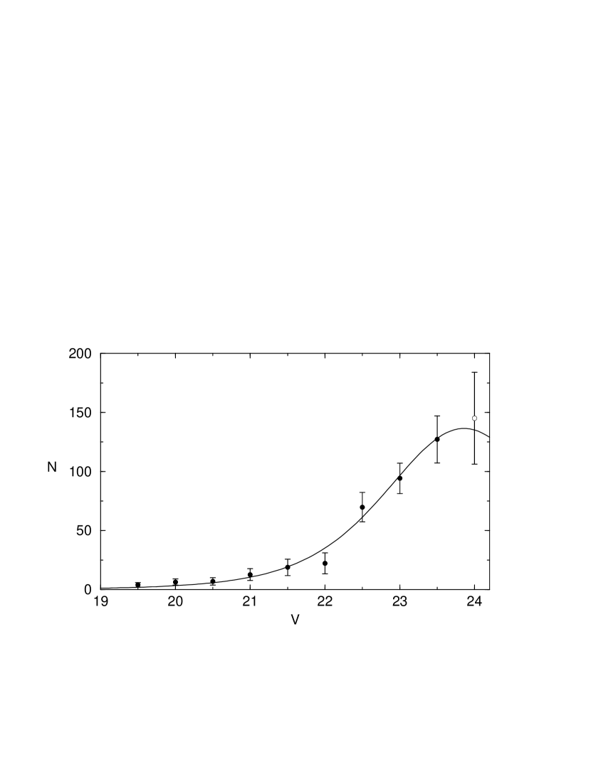
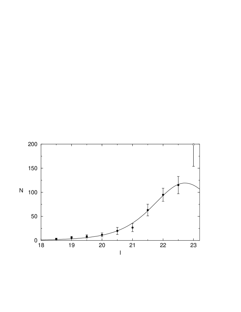
Figure 14: The luminosity functions for $B$, $V$ and $I$. The bin size is $0.5$ mag. The last bin (open circle) was not used in the fit, as its center is beyond the limiting magnitude. The smooth curve is the fit of a $t_{5}$ function with $\sigma=1.1$.

Table 7: The turnover magnitudes for the complete sample, and the blue and red subsamples in $B$, $V$ and $I$.

Filter	TOM	TOMblue	TOMred
$B$	$24.69\pm 0.15$	$24.66\pm 0.29$	$24.82\pm 0.31$
$V$	$23.87\pm 0.20$	$23.99\pm 0.98$	$23.85\pm 0.28$
$I$	$22.72\pm 0.14$	$23.16\pm 0.47$	$22.49\pm 0.20$

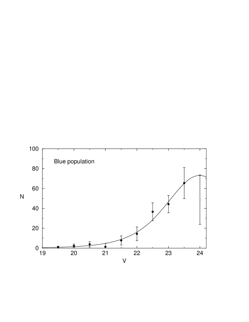
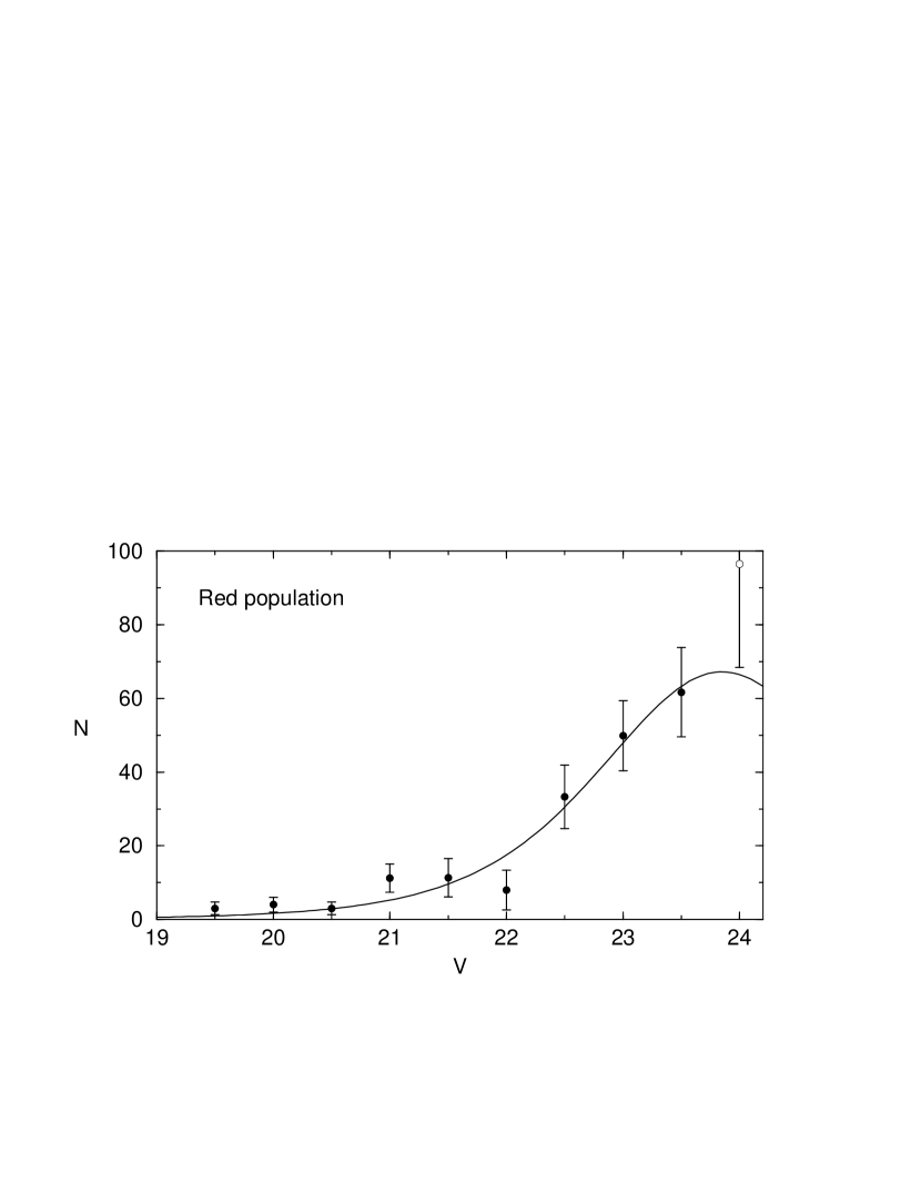
Figure 15: The GCLF of the blue and the red populations, in the $V$ band.

Table 8: Published TOMs for galaxies in the Fornax clusters, using the GCLF. References are as following: 1. Kohle et al. kohle96 (1996); 2. Blakeslee & Tonry blakeslee96 (1996); 3. Elson et al. elson98 (1998); 4. Della Valle et al. dellavalle98 (1998); 5. Ostrov et al. ostrov98 (1998); 6. Grillmair et al. grillmair99 (1999); 7. Richtler et al. richtler92 (1992).

Galaxy	TOM($B$)	TOM($V$)	TOM($I$)	Reference
NGC 1344		$23.80\pm 0.25$		2
NGC 1379	$24.95\pm 0.30$	$23.65\pm 0.26$	$22.77\pm 0.44$	1,3
NGC 1380	$24.38\pm 0.09$	$24.05\pm 0.25$		2,4
		$23.67\pm 0.11$		4
NGC 1399	$24.59\pm 0.10$	$23.83\pm 0.15$		2,6
		$23.90\pm 0.08$	$22.27\pm 0.05$	1
		$23.71\pm 0.12$		5
NGC 1404	$24.86\pm 0.21$	$24.10\pm 0.20$		6,7
		$23.92\pm 0.20$		2
NGC 1374		$23.44\pm 0.13$	$22.49\pm 0.12$	1
NGC 1427		$23.63\pm 0.19$	$22.22\pm 0.13$	1

4 Specific frequency

The specific frequency of a GCS is defined as the number of clusters per unit luminosity of the parent galaxy referred to $M_{V}=-15$ (Harris & van den Bergh harris81 (1981)): $S_{N}=N\cdot 10^{0.4\cdot(M_{V}+15)}$, where $N$ is the total number of clusters and $M_{V}$ the absolute $V$-magnitude of the host galaxy.

The basis for calculating $N$ is Table 5. We counted the number of globular clusters in each elliptical ring down to the TOM in $V$ (see Sects. 2.5 and 3.4).

The data in each ring were then corrected by the corresponding completeness function. When the rings were not fully covered by our frames (see Fig. 10), a geometrical correction factor was used to scale the counts to the total area. The results are listed in Table 5. The raw number of counts are listed in column 6. Column 7 lists the counts after the completeness correction. The geometrical factor is given in column 8. To calculate the total number of clusters in each annulus (column 9), we assumed the luminosity function to be symmetric around the TOM and doubled our counts. The total population of clusters (which includes background objects) was derived as the sum of the counts listed in column 9. The last three annuli were not included, as the counts cannot be distinguished from the background. Finally, to estimate the number of clusters in the central region (first annulus and inner ellipse) we extrapolated the data to follow the slope of the radial profile defined by the outer bins. This is because of the poor detection of clusters in this region, which would make the completeness correction too uncertain (see Fig. 5).

Several authors argue that tidal disruption and dynamical effects are more effective near the centre (for a discussion see e.g. Gnedin gnedin97 (1997)). Our purpose is to show that even if the central GCs were not affected by these destruction mechanisms, the specific frequency is still very low.

We then arrived at a mean density of $160\pm 30$ objects/$\squareforqed\arcmin$ down to the TOM for the innermost bin and inner ellipse. Thus, for this region of area $1.407\squareforqed\arcmin$, $225\pm 42$ clusters brighter than the TOM are expected. As with the outer bins, we doubled our counts around the TOM to obtain $N_{\rm annulus}=450\pm 84$.

Summing up the results for each annulus gives $1314\pm 240$ (see column 9 of Table 11). From this, one only needs to subtract the background counts, estimated to be $2.0$ objects/$\squareforqed\arcmin$. As we considered the geometrical incompleteness of the last three bins (see Fig. 10 and column 8 in Table 11), the total area of counting is $35.186\squareforqed\arcmin$ including the nucleus. Therefore, about $141$ background objects are to be subtracted. Again, the counts were doubled around the TOM. Finally, we estimate $N_{T}=1173\pm 240$ as the total population of clusters in NGC 1316.

With $\mu=31.35$ (Richtler et al. richtler00 (2000)) and an apparent magnitude $m_{V}=8.53$ (de Vaucouleurs et al. devaucouleur91 (1991)), we obtain $S_{N}=0.9\pm 0.2$, where the uncertainty results from error propagation and has the form:

$$\sigma=10^{0.4\cdot(M_{V}+15)}\sqrt{\sigma_{N}^{2}+(0.4\cdot N\cdot\ln 10)^{2}\cdot\sigma_{M_{V}}^{2}}$$ (6)

This is an extremely low value for a bright early-type galaxy. As we discuss below, it may result from the fact that the dominant light contribution to NGC 1316 comes from an intermediate age population instead from an old one. A similar interpretation has already been made by Hilker & Kissler-Patig (hilker96 (1996)) in the case of NGC 5018.

Furthermore, if one assumes that, due to dynamical effects, the surface density of the cluster population does not follow the power law, but tends to remain approximately constant in the two inner annuli, then the number of clusters drops to about 150, and the $S_{N}$ is decreased to 0.7.

Nevertheless, we cannot exclude the possibility of measuring an erroneous background density. As can be seen from the radial profile (Fig. 11), the background level is reached at $r\sim 300$ arcsec, where the average density is $2.0$ objects/$\squareforqed\arcmin$. It is interesting to investigate what are the effects of varying this number by $1\sigma$, as it enters directly into the Specific Frequency and hence, into the estimated age of the merger. This is discussed in Sect. 5.2.

5 Discussion

5.1 Subpopulations of clusters

The detection of intermediate-age clusters by Go00 clearly shows that the cluster system is inhomogeneous in terms of age. Also the strikingly different angular distributions of the blue and red clusters argues in favour of the existence of subpopulations. One would naturally assume that the red and probably metal-rich distribution, or part of it, has been formed in the merger. A popular scenario attributes the observed bimodal colour distributions in many early-type galaxies as being due to cluster formation in enriched gas during a merger (Ashman & Zepf ashmanzepf92 (1992), ashmanzepf97 (1997)). This bimodality is not seen in NGC 1316. However, we think that this is not of great significance, given the following points.

A bimodal metallicity distribution as a result of cluster formation during a merger probably needs special conditions. If, for example, the merger components were two spiral galaxies with a certain range of metallicities present in the gas content of their disks, then one naturally expects cluster formation with a similar range of metallicities, perhaps weighted to higher metallicities due to chemical enrichment during the merger. Any bimodal metallicity distribution, which has been present before the merger (and which does not stand in relation with the merger, like the bulge and disk clusters in the Milky Way), could well have been blurred.

Moreover, a metal-rich intermediate-age population of clusters, formed in the merger, for example with an age of 2 Gyr, would have $B-V$ colours which are about $0.2$  mag bluer than their old, metal-rich counterparts. According to the above relation between $B-I$ colour and [$\@element{\mathrm{Fe}}$/$\@element{\mathrm{H}}$], this corresponds to a metallicity difference of $0.5$ dex. The peak at $-0.8$ dex in Fig. 7 could well be explained in this way, comprised perhaps by clusters with solar metallicity and those found by Go00.

5.2 The Specific Frequency

Our result of $0.9\pm 0.2$ for the specific frequency of the GCLF of NGC 1316 confirms with a larger field what has been found by Gr99 using HST-data. This is an extremely low value for a bright, early-type galaxy, even more astonishing as one would expect to have many clusters formed during the merger process.

One possible explanation for this low value would be to assume that the merger caused, whether or not star clusters have been formed, a period of star formation, which nowadays constitute an intermediate-age population, which is brighter than an old population without strikingly differing in integral broad-band colours. The contribution of such a population could be visible spectroscopically by stronger hydrogen lines than normal.

We assume that a “normal” specific frequency of early-type galaxies is 4. The question then is: How young must NGC 1316 be to lower that value to our value of 0.9? Worthey (worthey94 (1994)) offers a tool for synthesizing stellar populations. Assuming a metallicity of $+0.5$ dex, we get from his “model interpolation engine” an age of 2 Gyr to account for the magnitude difference of $1.6$ mag in comparison to an old population of 15 Gyr.

The dominant error in this result is the uncertainty in the background density. If it were, instead of $2.0$ objects/$\squareforqed\arcmin$, $4.0$ objects/$\squareforqed\arcmin$, the total number of clusters decreases to $N_{T}=1033$ and $S_{N}=0.8$. On the other hand, a density of $0.0$ objects/$\squareforqed\arcmin$ implies $N_{T}=1314$ and $S_{N}=1.0$. Thus, a total error of $\sim 0.3$ results for $S_{N}$. This means, from Worthey’s models, an error in the age of the merger of $\sim$0.8 Gyr.

Our value of 2 Gyr is in good agreement with the luminosity-weighted mean stellar age of NGC 1316 given by Kuntschner & Davies (kuntschner98 (1998)), who measured line strengths for early-type galaxies in the Fornax cluster. It also matches the merger age of NGC 1316 estimated by Mackie & Fabbiano (mackie98 (1998)) and the globular cluster ages of Go00. In this context, one also should note that the occurence of two SNe Ia is a further indication for the existence of an intermediate-age population, to which many SNe Ia seem to belong (e.g. McMillan & Ciardullo mcmillan96 (1996)).

The question now arises whether specific frequencies of GCS in general could be influenced, if not dominated, by the existence of intermediate-age populations. One notes that among the sample of early-type galaxies, for which Trager et al. (trager2000 (2000)) measured age-sensitive line strengths, a few striking examples like NGC 221 or NGC 720 exist, which have a young component and whose specific frequencies are quite low for early-type galaxies. Another example is the merger candidate NGC 5018, for which Hilker & Kissler-Patig (hilker96 (1996)) found a low specific frequency, similar to that of NGC 1316, which they also explained by the presence of a young population.

A strong argument against the conjecture that this effect is dominating, is the fact that the specific frequency among early-type galaxies has a positive correlation with the environmental galaxy density (West west93 (1993)). If an enhanced number of mergers in a high density environment caused the existence of intermediate-age populations in many early-type galaxies, one would expect a negative correlation, if the brightness of the host galaxy significantly influenced the specific frequency. However, if the efficiency of globular cluster formation increases with the star formation rate, as the work of Larsen & Richtler (soeren00 (2000)) indicates, then a positive correlation, as observed, is understandable.

Larsen & Richtler (soeren00 (2000)) performed a survey of young clusters in a sample of 21 nearby face-on spiral galaxies. They found that the “specific luminosity” $T_{L}(U)$, which measures the ratio of the summed-up U-luminosity of cluster candidates to the total U-luminosity of the host galaxy, correlates well with indices measuring the star formation rate. Apparently, a high star formation rate causes also a higher cluster formation efficiency.

The final specific frequency after a merger therefore depends on many circumstances, among them the star formation rate, the amount of gas available for star formation, the specific frequency of the merger components, etc.

Can we expect that the merger enhances the specific frequency of the outcoming configuration? Go00 describe the evidence that makes NGC 1316 a candidate for an advanced disk-disk merger system. So let us assume that two spiral galaxies of equal brightness $M_{V}$ have merged.

If we set for the visual luminosity $L=10^{-0.4\cdot M_{V}}$ then the following relation holds:

$$N_{\mathrm{tot}}-N_{\mathrm{m}}=2\cdot 10^{-6}\cdot S_{N}\cdot L$$ (7)

with $N_{\mathrm{tot}}$ the total number of clusters, $N_{\mathrm{m}}$ the number of cluster formed in the merger, and $S_{N}$ the specific frequency of the merging spiral galaxies. Further:

$$L_{\mathrm{tot}}=2\cdot L_{\mathrm{dim}}+L_{\mathrm{m}}$$ (8)

where $L_{\mathrm{tot}}$ is the actual luminosity of NGC 1316, $L_{\mathrm{dim}}$ the actual luminosity of the former spirals, dimmed for about 3 Gyr, after star formation ceased, and $L_{\mathrm{m}}$ is the luminosity of the stellar population formed in the merger. A typical value for $S_{N}$ is 0.5 (Harris harris00 (2000)). $N_{\mathrm{m}}$ is not accurately known, but a rough estimate comes from the fact that Go00 found 3 clusters of masses comparable with $\omega$ Cen, so a lower boundary is 300 clusters. With these numbers, the luminosity of the hypothetical spirals, at the time of merging, turns out as $9\cdot 10^{8}$, corresponding to $M_{V}=-22.4$. The dim factor during the next 3 Gyr is about 2, based on a simulation with Worthey’s “model interpolation engine”. If $L_{\mathrm{tot}}$ is $1.32\cdot 10^{9}$, then $L_{\mathrm{m}}$ turns out as $4.2\cdot 10^{8}$, corresponding to $M_{V}=-21.6$. The stellar population formed in the merger will dim for 1.5 mag during the next 12 Gyr. The further fading of the spiral will be roughly by factor of 5, corresponding to the ratio of 10 between the M/L values of a spiral and an elliptical galaxy. Thus the total luminosity after aging will be about $3\cdot 10^{8}$, which means $M_{V}=-21.2$ and a specific frequency of 4.

The numbers used in this exercise are uncertain, but it shows that the higher specific frequency of elliptical galaxies with respect to spirals can indeed plausibly be understood as the outcome from disk-disk mergers.

The example also shows that a merging scenario of an elliptical galaxy with a spiral leads to such high merger luminosities, that the gas mass consumed by the star formation in the merger cannot reasonably be brought in by a spiral galaxy. For instance, an elliptical with $M_{V}=-21.5$ and specific frequency 3 corresponds through the above relations to a spiral galaxy with $M_{V}=-21.2$ and a merger brightness of $M_{V}=-22.4$. A population of this brightness with an age of 3 Gyr has a mass of almost $8\cdot 10^{10}\,M_{\odot}$, which cannot be provided by any ordinary-sized spiral.

It is, however, doubtful, whether high specific frequencies (6 and more) can be created by the merging of two or more spiral galaxies (Harris harris00 (2000)). It is more likely that dwarf galaxies must be involved if cluster systems like those of NGC 1399 and M87 are to be formed (Hilker et al. hilker99 (1999)).

5.3 The Luminosity Function

The importance of the LF of NGC 1316 lies in the fact that it could provide an accurate distance to the two SNe Ia SN 1980N and SN 1981D and thus help to calibrate the absolute SN Ia luminosity, as has been the case for SN 1992A in NGC 1380 (Della Valle et al. dellavalle98 (1998)).

However, due to its presumed merger history, one might suspect that the GCS of NGC 1316 is contaminated by younger clusters, which very probably should be searched for among the red cluster population. Broad band colours are not very sensitive: a cluster becomes redder in $V-I$ by only $0.2$ mag, evolving from an age of 2 Gyr to an age of 15 Gyr.

Such a contamination would also affect the turnover magnitude. OT95 investigated the evolution of a GCS considering the dynamical and photometric evolution of individual clusters. According to their results, the TOM would brighten by about $0.6$–$1.0$ mag, when a GCS evolves from an age of 2 Gyr to an age of 15 Gyr. Therefore one expects the TOM of the red cluster population to be fainter than that of the blue population, if the red clusters are indeed younger.

This has to be proved/disproved with deeper data than those at our disposal. Since the TOM is not reached in either among the red population or the blue population, its numerical value returned by the fit is rather uncertain and hence we cannot make any secure statement.

From the models of OT95, we would expect to see the TOM approximately at $V=24.5$ or $B=25.5$ in case that the majority of the red clusters has been formed in the merger.

Gr99, in a small field near the centre of NGC 1316, obtained $B$-photometry with HST to faint magnitudes. Their results are not easy to interpret. Their actual background-corrected and completeness-corrected counts do not rule out a turnover at $B=25.5$, but no turnover is indicated in their $I$-counts at $I=23.7$, where one expects it to be due to the mean $B-I$ colour of 1.8. If they correct for the contribution of “dust-obscured” objects, the resulting LF is completely dominated by the unseen population and there is a steady increase in both $B$ and $I$ down to the faintest magnitudes.

Gr99 conjecture that they see a population of open clusters, which is plausible if the star formation near the center has continued for some time after the merger. One can imagine that most of the globular clusters formed during the merger, when the star formation rate was high, but less massive open clusters continued to form at lower rate, which would blur the luminosity function of the globular clusters.

No detailed picture follows from the present data, but it is not excluded that a large fraction of the red globular clusters formed during the merger. Another (unknown) part may have been brought in by the merger components. If two spiral galaxies have merged they could have brought in their metal-rich bulge populations. The blue globular clusters would then be the common halo globular clusters of the two merger components. Star formation near the centre continued and younger star clusters were added to the cluster population formed during the merger. In that case, we would expect the outer population of red clusters to exhibit a TOM in the range 0.6 to 1 mag fainter than the blue cluster population, which could be shown by deeper photometry than we have.

In this scenario one should only regard the LF of the blue cluster population as appropriate for distance estimation.

5.4 A remark on the supernovae in NGC 1316

Two SNe of type Ia, SN 1980N and SN 1981D, appeared in NGC 1316 (Hamuy et al. hamuy91 (1991)). The distance determined by its GCLF can thus contribute to the calibration of the absolute peak brightness of SN Ia. There are only a handful of nearby early-type host galaxies for Ia supernovae, so NGC 1316 occupies an important role.

However, our data are not deep enough to measure the distance via the GCLF so accurately that SN 1980N could be independently compared with SN 1992A in NGC 1380, the third SN Ia which appeared in the Fornax cluster, and which has a very well measured GCLF (Della Valle et al. dellavalle98 (1998)). SN 1981D has a light curve of lower quality.

As Tables 7 and 8 show, the TOM of the GCS of NGC 1316 fits at least well to the other TOMs of early-type Fornax galaxies. This may be taken as an argument that NGC 1316, in spite of its outlying location, is in the same distance as the core of the Fornax cluster.

Indeed, after the appropriate corrections for decline-rate and colour (e.g. Hamuy et al. hamuy96 (1996), Richtler et al. richtler00 (2000)), the apparent peak brightness of SN 1980N agrees excellently with that of SN 1992A, which is a much stronger argument for their equal distance.

- (1) Ashman K.M., Zepf S.E., 1992, ApJ 384, 50
- (2) Ashman K.M., Zepf S.E., 1997, Globular Cluster Systems, Cambridge University Press
- (3) Bertin E., Arnouts S., 1996, A&AS 117, 393
- (4) Blakeslee J.P., Tonry J.L., 1996, ApJ 465, L19
- (5) Burstein D., Heiles C., 1982, AJ 87, 1165
- (6) Couture J., Harris W.E., Allwright J.W.B., 1990, ApJS 73, 671
- (7) de Vaucouleurs G., et al., 1991, Third Reference Catalogue of bright galaxies, Springer
- (8) Della Valle M., Kissler-Patig M., Danziger J., Storm J., 1998, MNRAS 299, 267
- (9) Drenkhahn G., Richtler T., 1999, A&A 349, 877
- (10) Elson R.A.W., Grillmair C.J., Forbes D.A., et al., 1998, MNRAS 295, 240
- (11) Ferrarese L., Mould J.R., Kennicutt R.C., et al., 2000, ApJ 529, 745
- (12) Gnedin O.Y., 1997, ApJ 487, 663
- (13) Goudfrooij P., Mack J., Kissler-Patig M., et al., 2000, MNRAS, in press. (Go00)
- (14) Grillmair C.J., Forbes D.A., Brodie J.P., Elson R.A., 1999, AJ 117, 167 (Gr99)
- (15) Hamuy, M., Phillips, M.M., Maza, J., et al., 1991, AJ 102, 208
- (16) Hamuy, M., Phillips, M.M., Schommer, R.A., et al., 1996, AJ 112, 2391
- (17) Harris W.E., van den Bergh S., 1981, AJ 86, 1627
- (18) Harris W.E., Pudritz R.E., 1994, ApJ 429, 177
- (19) Harris W.E., 2000, Globular Cluster Systems: Lectures for the 1998 Saas-Fee Advanced Course on Stars Clusters. Springer, in press.
- (20) Hilker M., Kissler-Patig M., 1996, A&A 314, 357
- (21) Hilker, M., Infante, L., Richtler, T., 1999, A&AS 138, 55
- (22) Holtzman J.A., Faber, S.M., Shaya, E.J., et al., 1992, AJ 103, 691
- (23) Jedrzejewski R.I., 1987, MNRAS 226, 747
- (24) Kissler-Patig M., Kohle S., Hilker M., et al., 1997, A&A 319, 470
- (25) Kissler-Patig M., Richtler T., Storm J., della Valle M, 1997, A&A 327, 503
- (26) Kohle S., Kissler-Patig M., Hilker M., et al., 1996, A&A 309, L39
- (27) Kuntschner H., Davies R.L., 1998, MNRAS 295, L29
- (28) Kuntschner H., 2000, MNRAS, in press (astro-ph/0001210)
- (29) Landolt A.U., 1992, AJ 104, 340
- (30) Larsen S.S., Richtler T., 1999, A&A 345, 59
- (31) Larsen S.S., Richtler T., 2000, A&A 354, 836
- (32) Mackie G., Fabbiano G., 1998, AJ 115, 514
- (33) McLaughlin D.E., Pudritz R.E., 1996, ApJ 457, 578
- (34) McMillan, R.J., Ciardullo, R., 1996, ApJ 473, 707
- (35) Miller B.W., Whitmore B.C., Schweizer F., Fall S.M., 1997, AJ 114, 2381
- (36) Okazaki T., Tosa M., 1995, MNRAS 274, 48 (OT95)
- (37) Ostrov P.G., Forte J.C., Geisler D., 1998, AJ 116, 2854
- (38) Poulain P., 1988, A&AS 72, 215
- (39) Richtler T., Grebel E.K., Domgoergen H., Hilker M., Kissler M., 1992, A&A 264, 25
- (40) Richtler T., Drenkhahn G., Gómez M., Seggewiss W., 1999, in: Science in the VLT Era and Beyond. ESO VLT Opening Symposium, Springer, in press (astro-ph/9905080)
- (41) Richtler T., Jensen J., Tonry J, Barry B., Drenkhahn G., 2000, in press.
- (42) Schweizer F., 1980, ApJ 237, 303
- (43) Schweizer F., 1981, ApJ 246, 722
- (44) Secker J., Harris W.E., 1993, AJ 105, 1358
- (45) Stetson P.B., 1990, PASP, 102, 932
- (46) Trager S.C., Faber S.M., Worthey G., Jesús Gonzáles J., 2000, AJ 119, 1645
- (47) West, M.J., 1993, MNRAS 265, 755
- (48) Whitmore B.C., Schweizer F., Leitherer C., Borne K., Robert C., 1993, AJ 106, 1354
- (49) Whitmore B., Sparks W.B., Lucas R.A., Macchetto F.D., Biretta J.A., 1995, ApJ 454, L73
- (50) Whitmore B.C., Schweizer F., 1995, AJ 109, 960
- (51) Worthey G., 1994, ApJS 95, 107, http://astro.sau.edu/∼worthey