Constraining the Cosmological Parameters using Strong Lensing

We investigate the potentiality of using strong lensing clusters to constrain the cosmological parameters $\Omega_{m}$ and $\Omega_{\lambda}$. The existence of a multiple image system with known redshift allows, for a given ($\Omega_{m}$, $\Omega_{\lambda}$) cosmology, absolute calibration of the total mass deduced from lens modelling. Recent Hubble Space Telescope (HST) observations of galaxy clusters reveal a large number of multiple images, which are predicted to be at different redshifts. If it is possible to measure spectroscopically the redshifts of many multiple images then one can in principle constrain ($\Omega_{m}$, $\Omega_{\lambda}$) through ratios of angular diameter distances, independently of any external assumptions. For a regular/relaxed cluster observed by HST with 3 multiple image systems, each with different spectroscopic redshifts, we show by analytic calculation that the following uncertainties can be expected: $\Omega_{m}=0.30\ \pm 0.11$, $\Omega_{\lambda}=0.70\ \pm 0.23$ or $\Omega_{m}=1.00\ \pm 0.17$, $\Omega_{\lambda}=0.00\ \pm 0.48$ for the two most popular world models. Numerical tests on simulated data confirm these good constraints, even in the case of more realistic cluster potentials, such as bimodal clusters, or when including perturbations by galaxies. To investigate the sensitivity of the method to different mass profiles, we also use an analytic “pseudo-elliptical” Navarro, Frenk & White profile in the simulations. These constraints can be improved if more than 3 multiple images with spectroscopic redshifts are observed, or by combining the results from different clusters. Some prospects on the determination of the cosmological parameters with gravitational lensing are given.

1 Introduction

A new “standard cosmological model” has arisen in the last few years, favoring a flat Universe with $\Omega_{m}\sim 0.3$ and $\Omega_{\lambda}\sim 0.7$. This is mainly based on the results of two experiments which give roughly orthogonal constraints in the $(\Omega_{m},\Omega_{\lambda})$ plane (see Fig. 1 for a recent update). The first one is obtained by considering type Ia supernovae (SNIa) as standard candles. The detection of a sample of high redshift SNIa (up to $z\sim$ 1) by two groups favours a non-vanishing cosmological constant (Perlmutter et al., 1998; Riess et al., 1998), large enough to produce an accelerating expansion. However, evidence for a non-zero cosmological constant is still controversial, since supernovae might evolve with redshift and/or may be dimmed by intergalactic dust (Aguirre, 1999). The fundamental assumption of a homogeneous Universe and its implication for a non-zero cosmological constant are also discussed (Célérier, 2000; Kolatt & Lahav, 2001). The second constraint is derived from the location of features in the cosmic microwave background (CMB) anisotropy spectrum, particularly the first Doppler peak. The most recent results obtained with the Boomerang and MAXIMA experiments favor a flat Universe (Balbi et al., 2000; Melchiorri et al., 2000). However, there still remains a degeneracy in the combination of $\Omega_{m}$ and $\Omega_{\lambda}$ because CMB experiments are primarily sensitive to the total curvature of the Universe. Even with the accuracy of the future MAP and Planck missions, the constraint issued from the CMB alone will be degenerate.

The combination of these two sets of constraints has led to the currently favored model of low matter density and a non-zero cosmological constant, preserving a flat geometry (e.g. White, 1998; Efstathiou et al., 1999; Freedman, 2000; Sahni & Starobinsky, 2000; Jaffe et al., 2001). Although these recent results are quite spectacular, there still remain many sources of uncertainties with both methods. Thus any other independent test to constrain the large scale geometry of the Universe is important to investigate. Gravitational lensing, an effect involving large distance scales, has been considered as a very promising tool for such determinations. Indeed, the statistics of gravitational lenses depend on the cosmological parameters via angular size distances and the comoving spherical volume (e.g. Turner et al., 1984; Turner, 1990; Kochanek, 1996; Falco et al., 1998). This technique has provided an upper limit on $\Omega_{\lambda}$ using different surveys of galaxy lens systems: multiple quasar statistics (Kochanek, 1996; Chiba & Yoshii, 1999), lensed radio sources (Cooray, 1999), lensed galaxies in the Hubble Deep Field (Cooray et al., 1999). Although most authors favor a lambda-dominated flat Universe, there remain some uncertainties in the mass distribution of the galaxy lenses and on the luminosity function of the sources. Evolutionary effects may also play a role in these statistics.

Another application of gravitational lensing to constrain the cosmological parameters is to use the statistics of the “cosmic” shear variance. Van Waerbeke et al. (1999) showed that it is related to the power spectrum of the large scale mass fluctuations, and then to $\Omega_{m}$. The first results of deep wide field imaging surveys favor $\Omega_{m}$ in the range [0.2–0.5] (Maoli et al., 2001; Van Waerbeke et al., 2001; Bacon et al., 2000; Wittman et al., 2000). Imaging surveys with the next generation of panoramic CCD cameras will reinforce this very promising technique. In the case of weak lensing by clusters of galaxies, Lombardi & Bertin (1999) and Gautret et al. (2000) suggested methods to constrain the geometry of the Universe. These methods need however to recover the mass distribution and/or to know acurately the redshift of a huge number of distant galaxies, making this method not practical in the near future.

In this paper, we focus on a measurement technique of $(\Omega_{m},\Omega_{\lambda})$ using gravitational lensing as a purely geometrical test of the curvature of the Universe, since the lens equation depends on the ratio of angular size distances which is sensitive to the cosmological parameters. In the most favorable case, a massive cluster of galaxies can lens several background galaxies, splitting the images into several families of multiple images. The existence of one family of multiple images, at known redshift, allows to calibrate the total cluster mass in an absolute way. In the case of several sets of multiple images with known redshifts, it is possible in principle to constrain the geometry of the Universe. This method was pointed out by Blandford & Narayan (1992), and earlier suggested by Paczynski & Gorski (1981), but the uncertainties in any lens studies were considered too large compared to the small variations induced by the cosmological parameters. More recently, Link & Pierce (1998) (hereafter LP98) re-analysed the question in the light of the typical accuracy reached with HST images of clusters of galaxies. Following their method, which inspired our work, we try to quantify in this paper what can be reasonably obtained on $(\Omega_{m},\Omega_{\lambda})$ from accurate lens modeling of realistic cluster-lenses.

The paper is organized as follows. In Sect. 2 we summarize the main lensing equations and we introduce the relevant angular size distance ratio which contains the dependence on the cosmological parameters. The variation of this ratio is then compared to that of other variables (lens potential parameters and redshifts) to derive the expected uncertainties on $\Omega_{m}$ and $\Omega_{\lambda}$. In Sect. 3 we present the method in detail and the results from simulations of various types of families of images and of different types of lens potentials. Some conclusions and prospects for the application to real data are discussed in Sect. 4. Throughout this paper we assume $H_{0}=65$ km s^-1 Mpc^-1 (note however that the proposed method and results are independent of $H_{0}$).

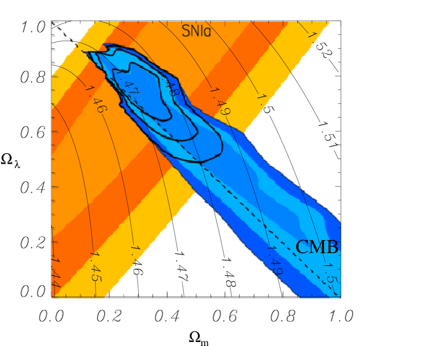
Figure 1: Constraints on $(\Omega_{m},\Omega_{\lambda})$ derived from the most recent results of the BOOMERANG and MAXIMA-I experiments on the CMB fluctuations and the last results from the SNIa analysis (from Jaffe, 2001). Overplotted is the ratio of the geometrical factor of the lens equation for two source redshifts, $e(z_{S1},z_{S2})=E(z_{S1})/E(z_{S2})$ as discussed in the text. In this example, the redshifts are chosen as representative of a typical lens configuration: $z_{\mathrm{L}}=0.3$, $z_{S1}=0.7$ and $z_{S2}=2$.

2 Influence of $\Omega_{m}$ and $\Omega_{\lambda}$ on image formation

2.1 Cosmology dependent lensing relations

We first define the basic mathematical framework, following the formalism presented in Schneider et al. (1992). We consider a lens at a redshift $z_{\mathrm{L}}$ with a two-dimensional projected mass distribution $\Sigma(\@vec{\theta})$ and a projected gravitational potential $\phi(\@vec{\theta})$, where $\@vec{\theta}$ is a two-dimensional vector representing the angular position. A source galaxy with redshift $z_{\mathrm{S}}$ is located at position $\@vec{\theta_{S}}$ in the absence of a lens, and its image is at position $\@vec{\theta_{I}}$. In the lens equation

$$\left\{\begin{array}[]{l}\@vec{\theta_{S}}=\@vec{\theta_{I}}-\@vec{\nabla}\varphi(\@vec{\theta_{I}})\\ \varphi(\@vec{\theta})=\displaystyle{\frac{2}{c^{2}}}\displaystyle{\frac{D_{\mathrm{LS}}}{D_{\mathrm{OL}}D_{\mathrm{OS}}}}\phi(\@vec{\theta}),\end{array}\right.$$ (1)

$D_{\mathrm{OL}}$, $D_{\mathrm{LS}}$ and $D_{\mathrm{OS}}$ are respectively the angular diameter distances from the Observer to the Lens, from the Lens to the Source and from the Observer to the Source (Peebles, 1993). $\varphi$ is the reduced gravitational potential which satisfies $\nabla^{2}\varphi=2\ \Sigma/\Sigma_{\rm crit}$ with the critical density

$$\Sigma_{\rm crit}=\displaystyle{\frac{c^{2}}{4\pi G}}\displaystyle{\frac{D_{\mathrm{OS}}}{D_{\mathrm{LS}}D_{\mathrm{OL}}}}.$$ (2)

In these equations the dependence on the cosmological parameters appears only through the angular diameter distances ratios $F=\displaystyle{\frac{D_{\mathrm{OL}}\ D_{\mathrm{LS}}}{D_{\mathrm{OS}}}}$ and $E=\displaystyle{\frac{D_{\mathrm{LS}}}{D_{\mathrm{OS}}}}$ ($E$ as “efficiency”) for a fixed cluster redshift. They correspond to a scaling of the lens equation, reflecting the geometrical properties of the Universe.

In the general case, we can scale the potential gradient as:

$$\@vec{\nabla}\phi(\@vec{\theta_{I}})=\sigma_{0}^{2}\ D_{\mathrm{OL}}\ \@vec{f}(\@vec{\theta_{I}},\theta_{C},\alpha,\ldots)$$ (3)

where $\sigma_{0}$ is the central velocity dispersion and $\@vec{f}$ a dimensionless function that describes the mass distribution of the cluster. It can be represented by fiducial parameters such as a core radius $\theta_{C}$ or a mass profile gradient $\alpha$. The lens equation reads

$$\@vec{\theta_{S}} = \@vec{\theta_{I}}-\frac{\sigma_{0}^{2}}{c^{2}}\ \frac{D_{\mathrm{LS}}}{D_{\mathrm{OS}}}\ \@vec{f}(\@vec{\theta_{I}},\theta_{C},\alpha,\ldots)$$

$$= \@vec{\theta_{I}}-\frac{\sigma_{0}^{2}}{c^{2}}\ \@vec{f}(\@vec{\theta_{I}},\theta_{C},\alpha,\ldots)\times E(\Omega_{m},\Omega_{\lambda},z_{\mathrm{L}},z_{\mathrm{S}})$$

We will focus on the $E$-term which entirely contains the dependence on $\Omega_{m}$ and $\Omega_{\lambda}$ and which is independent of $H_{0}$.

2.2 The E-term

For a given lens plane $z_{\mathrm{L}}$, the ratio $E$ increases rapidly as the source redshift increases, and then flattens at $z_{\mathrm{S}}\sim 1.5$. There are also small but significant changes with the cosmological parameters (Fig. 2). The dependence of $E$ with respect to $\Omega_{m}$ is weak, whereas the variation with $\Omega_{\lambda}$ is larger.

We now consider fixed redshifts for the lens and sources. Assuming a fixed world model, a single family of multiple images can in principle constrain the total cluster mass as well as the shape of the potential, removing the unknown position of the source $\@vec{\theta_{S}}$ using Eq.(2.1). In practice, good constraints on the shape of the potential $\@vec{f}$ are obtained with triple, quadruple or quintuple image systems. However the absolute normalization $\sigma_{0}$ of the mass is degenerate with the E-term, that is with respect to $\Omega_{m}$ and $\Omega_{\lambda}$.

Figure 2: Variation of the lens efficiency $E(z_{\mathrm{S}})$ as a function of the source redshift for different sets of cosmological parameters:. (Left): $\Omega_{\lambda}=0$ and $\Omega_{m}$ varies from 0.1 to 1.0. (Right): $\Omega_{m}=0.3$ and $\Omega_{\lambda}$ varies from 0 to 0.7. In both cases, the lens redshift is $z_{\mathrm{L}}=0.3$. For clarity, above each main plot, we also plotted the same curves, normalised with the $E(z_{\mathrm{S}})$ function for $(\Omega_{m},\Omega_{\lambda})=(0.3,0.)$.

2.3 Ratio of E-terms for 2 sets of source redshifts

To break this degeneracy a second family of multiple images is needed. To get rid of the strong dependence on $\sigma_{0}$, it is useful to consider the ratio of the positions:

$$\frac{\|\@vec{\theta_{I_{1}^{1}}}-\@vec{\theta_{I_{2}^{1}}}\|}{\|\@vec{\theta_{I_{1}^{2}}}-\@vec{\theta_{I_{2}^{2}}}\|}=\frac{E(z_{S1})\|\@vec{f}(\@vec{\theta_{I^{1}_{1}}},\ldots)-\@vec{f}(\@vec{\theta_{I^{1}_{2}}},\ldots)\|}{E(z_{S2})\|\@vec{f}(\@vec{\theta_{I^{2}_{1}}},\ldots)-\@vec{f}(\@vec{\theta_{I^{2}_{2}}},\ldots)\|}$$ (5)

(here and hereafter, the superscript refers to a family and the subscript to a particular image within a family). This ratio is plotted in Fig. 1, highlighting the influence of $\Omega_{m}$ and $\Omega_{\lambda}$ through the ratio $\displaystyle e(z_{S1},z_{S2})=E(z_{S1})/E(z_{S2})$.

Note that the discrepancy between the different cosmological parameters is not very large, less than 3% between the Einstein-de Sitter model (EdS) and a flat, low matter density one. Moreover, a characteristic degeneracy appears in the $(\Omega_{m},\Omega_{\lambda})$ plane, which is roughly orthogonal to the one given by the detection of high redshift supernovae, and quite different from the CMB constraints. A similar degeneracy was also found in the analog weak lensing analyses, (Lombardi & Bertin, 1999) or by Gautret et al. (2000).

Another approach to quantify the dependence of a given lens configuration on $\Omega_{m}$ and $\Omega_{\lambda}$ is to fix the lens redshift and to search for two source redshifts $z_{S1}$ and $z_{S2}$ which give the largest variation of the $E$-term when scanning the $(\Omega_{m},\Omega_{\lambda})$ plane. For illustration we arbitrarily choose two sets of cosmological parameters, for which the relative variation of $E$ is large: CP1 $(\Omega_{m}=0.3,\Omega_{\lambda}=0)$ and CP2 ($\Omega_{m}=1,\Omega_{\lambda}=0$, i.e. the EdS model). Varying $z_{S1}$ and $z_{S2}$, the function $\varepsilon(z_{S1},z_{S2})=e_{CP2}(z_{S1},z_{S2})/e_{CP1}(z_{S1},z_{S2})-1$ represents the percentage of discrepancy between $CP1$ and $CP2$ for $z_{S1}\geq z_{S2}\ (\geq z_{\mathrm{L}})$ (Fig. 3).

For a given high-redshift $z_{S2}$ source the best lowest source redshift is $z_{S1}\simeq z_{\mathrm{L}}$, and for a given $z_{S1}$ the best $z_{S2}$ is the highest redshift, the difference between cosmological models increasing with $z_{S2}$. In all cases, this relative difference is of the order of a few %, meaning that the lens mass distribution must be known to the same degree of accuracy to get further constraints on the cosmological parameters. Hence, for 2 systems of images, the best configuration is one background source close to the lens, in the rising part of $E(z_{\mathrm{S}})$ and another one at high redshift, to take into account the asymptotic value of the ratio. Note however that for a source redshift close to the lens, the $E$-term becomes very small. Also, the location of the images is very close to the lens center which makes the detection of multiple images quite improbable, as small caustic sizes imply small cross sections.

Figure 3: Relative difference between the ratio $e(z_{S1},z_{S2})=E(z_{S1})/E(z_{S2})$ for two extreme cosmological models: $(\Omega_{m}=0.3,\Omega_{\lambda}=0)$ and ($\Omega_{m}=1,\Omega_{\lambda}=0$). This function $\varepsilon(z_{S1},z_{S2})$ is plotted in the $(z_{S1},z_{S2})$ plane, assuming $z_{S1}\leq z_{S2}$ and $z_{\mathrm{L}}=0.3$.

2.4 Relative influence of the lens parameters

2.4.1 Physical assumptions

In order to quantify the expected uncertainties on $\Omega_{m}$ and $\Omega_{\lambda}$, it is possible to analytically estimate the influence of the different lens models parameters. We use a model of the potential derived from the mass density described by Hjorth & Kneib (2001), hereafter HK. It is based on a physical scenario of violent relaxation in galaxies, also valid in clusters of galaxies. The mass density is characterized by a core radius $a$ and a cut-off radius $s$:

$$\rho(r)=\frac{\rho_{0}}{\left(1+\frac{r^{2}}{a^{2}}\right)\left(1+\frac{r^{2}}{s^{2}}\right)}.$$ (6)

Then the projected mass density $\Sigma(\theta)$ is represented by:

$$\Sigma(\theta)=\Sigma_{0}\ \frac{\theta_{a}\theta_{s}}{\theta_{s}-\theta_{a}}\ \left(\frac{1}{\sqrt{\theta^{2}+\theta_{a}^{2}}}-\frac{1}{\sqrt{\theta^{2}+\theta_{s}^{2}}}\right),$$ (7)

where $\theta$ is the angular coordinate, $\theta_{a}=a/D_{\mathrm{OL}}$ and $\theta_{s}=s/D_{\mathrm{OL}}$. $\Sigma_{0}$ is a normalization factor, related to the cluster parameters:

$$\Sigma_{0}=\pi\rho_{0}D_{\mathrm{OL}}\ \frac{\theta_{a}\theta_{s}}{\theta_{s}+\theta_{a}}.$$ (8)

Finally,the mass inside the projected angular radius $\theta$ is:

$$M(\theta) = 2\pi\Sigma_{0}D_{\mathrm{OL}}^{2}\ \frac{\theta_{a}\theta_{s}}{\theta_{s}-\theta_{a}}\times$$ (9)

$$\quad\left[\sqrt{\theta^{2}+\theta_{a}^{2}}-\sqrt{\theta^{2}+\theta_{s}^{2}}+\theta_{s}-\theta_{a}\right].$$

The velocity dispersion $\sigma(\theta)$ is related to the mass density and the gravitational potential via the Jeans equation. Assuming an isotropic velocity dispersion and retaining terms up to first order in $\theta_{a}/\theta_{s}$, we get the relation between the central velocity dispersion $\sigma_{0}=\sigma(0)$ and $\rho_{0}$:

$$\sigma_{0}^{2}=\frac{\pi^{3}Ga^{2}}{2}\ \rho_{0}s.$$ (10)

Finally we compute the expression of the deviation angle between the positions of the source and of the image due to the lens: $D_{\theta_{I}}=\|\@vec{\theta_{I}}-\@vec{\theta_{S}}\|$, neglecting second order terms in $\theta_{a}/\theta_{s}$ (we suppose here $s\gg a$):

$$D_{\theta_{I}}=\frac{16}{\pi}\frac{\sigma_{0}^{2}}{c^{2}}\,E\,\frac{1}{\theta_{I}}\left[\sqrt{\theta^{2}+\theta_{a}^{2}}-\sqrt{\theta^{2}+\theta_{s}^{2}}+\theta_{s}-\theta_{a}\right].$$ (11)

2.4.2 The single multiple-image configuration

The central velocity dispersion (or equivalently the mass normalization of the cluster core) is obviously the predominant factor in any lens configuration. With a single family of images we can only constrain the combination $\sigma_{0}^{2}E$ and cannot disentangle the influence of the cosmological parameters and the absolute normalization of the mass (Fig. 4). If we were able to measure the total mass within the Einstein radius independently from lensing techniques and with an accuracy better than a few %, we could in principle put some constraints on $\Omega_{\lambda}$. Observationally, there are 2 situations where it is likely that we could disentangle the effect of cosmology and absolute mass:
1) in the case of a cluster-lens with extremely good X-ray data, particularly in estimating the temperature distribution of the gas (under the assumption of hydrostatic equilibrium),
2) in the case of a multiple system around a single galaxy, for which one is able to measure accurately the stellar velocity dispersion of the lensing galaxy (Tonry & Franx, 1999).
However in both cases this represents some observational challenge and requires the most powerful instruments to achieve this goal.

Figure 4: Variation of the central velocity dispersion $\sigma_{0}$ in the ($\Omega_{m},\Omega_{\lambda}$) plane, assuming that the product $\sigma_{0}^{2}E(z_{\mathrm{S}})$ is constant. $\sigma_{0}$ has been fixed to 1000 km s^-1 for $\Omega_{m}=1$, $\Omega_{\lambda}=0$ while $z_{\mathrm{L}}=0.3$ and $z_{\mathrm{S}}=1$.

Although the error budget in the image positions is dominated by the error on the total cluster mass (or equivalently the velocity dispersion), we can determine the relative influence of the other parameters to infer the importance of $\Omega_{m}$ and $\Omega_{\lambda}$ in the image formation. The relative error on the deviation angle $D_{\theta_{I}}$ depends on $\sigma_{0}$, $\theta_{a}$, $\theta_{s}$ and $\theta_{I}$ for the gravitational potential, and $z_{\mathrm{L}}$, $z_{\mathrm{S}}$, $\Omega_{m}$ and $\Omega_{\lambda}$ for the $E$-term (Eq.(11)). Therefore we can write:

$$\frac{\mathrm{d}D_{\theta_{I}}}{D_{\theta_{I}}}=\frac{\mathrm{d}E}{E}+\alpha_{\sigma_{0}}\frac{\mathrm{d}\sigma_{0}}{\sigma_{0}}+\alpha_{\theta_{a}}\frac{\mathrm{d}\theta_{a}}{\theta_{a}}+\alpha_{\theta_{s}}\frac{\mathrm{d}\theta_{s}}{\theta_{s}}+\alpha_{\theta_{I}}\frac{\mathrm{d}\theta_{I}}{\theta_{I}},$$ (12)

with

$$\frac{\mathrm{d}E}{E}(z_{\mathrm{S}})=\alpha_{\Omega_{m}}\frac{\mathrm{d}\Omega_{m}}{\Omega_{m}}+\alpha_{\Omega_{\lambda}}\frac{\mathrm{d}\Omega_{\lambda}}{\Omega_{\lambda}}+\alpha_{z_{\mathrm{L}}}\frac{\mathrm{d}z_{\mathrm{L}}}{z_{\mathrm{L}}}+\alpha_{z_{\mathrm{S}}}\frac{\mathrm{d}z_{\mathrm{S}}}{z_{\mathrm{S}}}.$$ (13)

$\alpha_{\theta_{a}}$, $\alpha_{\theta_{s}}$ and $\alpha_{\theta_{I}}$ can be computed analytically while $\alpha_{\sigma_{0}}=2$ is the largest factor. Since the angular diameter distances do not have an analytic expression if $\Omega_{\lambda}$ is non-zero, the coefficients $\alpha_{\Omega_{m}}$, $\alpha_{\Omega_{\lambda}}$, $\alpha_{z_{\mathrm{L}}}$ and $\alpha_{z_{\mathrm{S}}}$ must be computed numerically. In practise, they are computed for a given set of parameters $(z_{\mathrm{L}},\Omega_{m},\Omega_{\lambda})$ as their variation with $\Omega_{m}$ and $\Omega_{\lambda}$ is of higher order. For a reasonable set of lens parameters, the $\alpha$-coefficients are of the same order of magnitude, except that $\alpha_{z_{\mathrm{S}}}$ and $\alpha_{z_{\mathrm{L}}}$ can dominate the error budget if the source redshift is close to the lens (an unlikely case). On the contrary, $\alpha_{\Omega_{m}}$ and $\alpha_{\Omega_{\lambda}}$ are of second order, and $\alpha_{\Omega_{\lambda}}$ is somewhat larger than $\alpha_{\Omega_{m}}$. This reflects again the fact that $E$-term is more sensitive to $\Omega_{\lambda}$ than to $\Omega_{m}$.

To quantify the relative influence of all the parameters in the case of a single family of images, we computed explicitely $\mathrm{d}D_{\theta_{I}}/D_{\theta_{I}}$ in two cases, for a cluster-lens and for a galaxy-lens.

1) For a cluster of galaxies, we take the following parameters: $z_{\mathrm{L}}=0.3$, $z_{\mathrm{S}}=4$, $\Omega_{m}=0.3$, $\Omega_{\lambda}=0.7$, $\theta_{s}/\theta_{a}=10$ and $\theta_{I}/\theta_{a}=4$. We thus find from Eq.(11):

$$\frac{\mathrm{d}D_{\theta_{I}}}{D_{\theta_{I}}} = 2\,\frac{\mathrm{d}\sigma_{0}}{\sigma_{0}}-0.31\,\frac{\mathrm{d}\theta_{I}}{\theta_{I}}-0.21\,\frac{\mathrm{d}\theta_{a}}{\theta_{a}}+0.51\,\frac{\mathrm{d}\theta_{s}}{\theta_{s}}$$

$$- 0.17\,\frac{\mathrm{d}z_{\mathrm{L}}}{z_{\mathrm{L}}}+0.062\,\frac{\mathrm{d}z_{\mathrm{S}}}{z_{\mathrm{S}}}+0.012\,\frac{\mathrm{d}\Omega_{m}}{\Omega_{m}}+0.14\,\frac{\mathrm{d}\Omega_{\lambda}}{\Omega_{\lambda}}$$

Let us assume a perfectly known mass profile (i.e. d$\theta_{a}=\mathrm{d}\theta_{s}=0.$). Neglecting the influence of $\Omega_{m}$, we ask what precision would be required on $\sigma_{0}$ to derive an error of 50% on $\Omega_{\lambda}$. The accuracy of the position of the center of the images is calculated using the first moment of the flux $f(\theta)$ on a given image: $\theta_{I}=\int\theta f(\theta)\mathrm{d}\theta^{2}/\int f(\theta)\mathrm{d}\theta^{2}$ which yields an error $\mathrm{d}{\theta_{I}}$ of a fraction of the spatial resolution. HST observations are then required to reach $\mathrm{d}\theta_{I}=0.1\arcsec$ (LP98) or better. To reduce the uncertainty on the redshift measurements, we assume spectroscopic determinations, so that $dz\simeq 0.001$. Finally we have to compute the relative errors on $D_{\theta_{I}}=\|\@vec{\theta}_{I}-\@vec{\theta}_{S}\|$, so the position of the source is in principle required. But as we are in the strong lensing regime, we assume that $\theta_{S}\ll\theta_{I}$, so that both quantities $D_{\theta_{I}}\simeq\theta_{I}$ and $\displaystyle{\frac{\mathrm{d}D_{\theta_{I}}}{D_{\theta_{I}}}\simeq\frac{\mathrm{d}\theta_{I}}{\theta_{I}}}$ are directly related to observable ones. Taking these values into account, we need to know $\sigma_{0}$ with 3.6% accuracy to get the expected constraint on $\Omega_{\lambda}$. Such an accuracy is out of reach with observations of clusters of galaxies.

2) For a single galaxy, we consider typically: $z_{\mathrm{L}}=0.3$, $z_{\mathrm{S}}=4$, $\Omega_{m}=0.3$, $\Omega_{\lambda}=0.7$, $\theta_{s}/\theta_{a}=200$ and $\theta_{I}/\theta_{a}=200$ (ratios taken from the modelisation of the lens HST 14176+5226 by Hjorth & Kneib (2001)), leading to:

$$\frac{\mathrm{d}D_{\theta_{I}}}{D_{\theta_{I}}} = 2\,\frac{\mathrm{d}\sigma_{0}}{\sigma_{0}}-0.72\,\frac{\mathrm{d}\theta_{I}}{\theta_{I}}-0.0066\,\frac{\mathrm{d}\theta_{a}}{\theta_{a}}+0.73\,\frac{\mathrm{d}\theta_{s}}{\theta_{s}}$$

$$- 0.17\,\frac{\mathrm{d}z_{\mathrm{L}}}{z_{\mathrm{L}}}+0.062\,\frac{\mathrm{d}z_{\mathrm{S}}}{z_{\mathrm{S}}}+0.012\,\frac{\mathrm{d}\Omega_{m}}{\Omega_{m}}+0.14\,\frac{\mathrm{d}\Omega_{\lambda}}{\Omega_{\lambda}}$$

Taking the same values for the observational errors and considering a perfectly known mass profile, we require an accuracy of 6.4% on $\sigma_{0}$ to derive a 50% error on $\Omega_{\lambda}$. For a typical galaxy, this represents about 15 km s^-1. Warren et al. (1998) measured the velocity dispersion in the deflector of the Einstein ring 0047–2808 with an error of 30 km s^-1. A better accuracy could be obtained by looking at particular strong absorption features with 10m class telescope observations. This could be sufficient to confirm an accelerating Universe.

2.4.3 Configuration with 2 multiple-image systems

With a second system of multiple images another region of the $E(z_{\mathrm{S}})$ curve is probed while the cluster parameters are the same. In that case, the relevant quantity becomes the ratio of the deviation angles for 2 images $\theta_{I^{1}}$ and $\theta_{I^{2}}$ belonging to 2 different families at redshifts $z_{S1}$ and $z_{S2}$. We define $R_{\theta_{I^{1}},\theta_{I^{2}}}=\displaystyle{\frac{D_{\theta_{I^{2}}}}{D_{\theta_{I^{1}}}}}$. This function has the advantage that it does not depend on $\sigma_{0}$ anymore. Following our previous definitions, we can write

$$\frac{\mathrm{d}R_{\theta_{I^{1}},\theta_{I^{2}}}}{R_{\theta_{I^{1}},\theta_{I^{2}}}} = \frac{\mathrm{d}E(z_{S2})}{E(z_{S2})}-\frac{\mathrm{d}E(z_{S1})}{E(z_{S1})}$$ (16)

$$+ \alpha_{\theta_{I}}\left(\theta_{I^{2}}\right)\,\frac{\mathrm{d}\theta_{I^{2}}}{\theta_{I^{2}}}-\alpha_{\theta_{I}}\left(\theta_{I^{1}}\right)\,\frac{\mathrm{d}\theta_{I^{1}}}{\theta_{I^{1}}}$$

$$+ \Big{(}\alpha_{\theta_{a}}\left(\theta_{I^{2}}\right)-\alpha_{\theta_{a}}\left(\theta_{I^{1}}\right)\Big{)}\,\frac{\mathrm{d}\theta_{a}}{\theta_{a}}$$

$$+ \Big{(}\alpha_{\theta_{s}}\left(\theta_{I^{2}}\right)-\alpha_{\theta_{s}}\left(\theta_{I^{1}}\right)\Big{)}\,\frac{\mathrm{d}\theta_{s}}{\theta_{s}}$$

Numerically, we chose a typical configuration to compute $\displaystyle{\frac{\mathrm{d}R_{\theta_{I^{1}},\theta_{I^{2}}}}{R_{\theta_{I^{1}},\theta_{I^{2}}}}}$: $\theta_{s}/\theta_{a}=10$, $\theta_{I^{2}}/\theta_{a}=4$, $\theta_{I^{2}}/\theta_{I^{1}}=2$, $z_{\mathrm{L}}=0.3$, $z_{S1}=0.6$, $z_{S2}=5$, assuming $\Omega_{m}=0.3$ and $\Omega_{\lambda}=0.7$. This gives the following error budget:

$$\frac{\mathrm{d}R_{\theta_{I^{1}},\theta_{I^{2}}}}{R_{\theta_{I^{1}},\theta_{I^{2}}}} = 0.92\,\frac{\mathrm{d}z_{L}}{z_{L}}-0.99\,\frac{\mathrm{d}z_{S1}}{z_{S1}}+0.062\,\frac{\mathrm{d}z_{S2}}{z_{S2}}$$ (17)

$$- 0.018\,\frac{\mathrm{d}\theta_{I^{1}}}{\theta_{I^{1}}}-0.31\,\frac{\mathrm{d}\theta_{I^{2}}}{\theta_{I^{2}}}+0.12\,\frac{\mathrm{d}\theta_{a}}{\theta_{a}}$$

$$+ 0.21\,\frac{\mathrm{d}\theta_{s}}{\theta_{s}}+0.034\,\frac{\mathrm{d}\Omega_{m}}{\Omega_{m}}+0.037\,\frac{\mathrm{d}\Omega_{\lambda}}{\Omega_{\lambda}}$$

The contribution of the physical lens parameters in this error budget is strongly attenuated comprared to the single family case. There is no more dependence on $\sigma_{0}$ and the dependence on the mass profile ( $\theta_{a},\theta_{s}$) is reduced by about a factor of 2 compared to a single family of images. This corresponds to the variation of the potential between $\theta_{I1}$ and $\theta_{I2}$, the absolute normalization being removed. Anyhow, this can still represent the main source of error because we cannot expect to constrain $\theta_{a}$ to better than 1.5% and $\theta_{s}$ to better than 2% typically (see Sect. 3.3.3).

For the source redshifts, we have selected one of the sources at $z_{S1}=0.6$, which means that its $\alpha$-coefficient is quite large. The accurate value of the redshifts is thus fundamental, and a spectroscopic determination is essential ($dz\simeq 0.001$). A photometric redshift estimate would not be satisfactory, because we cannot expect an accuracy better than 10% in most cases ($\mathrm{d}z\simeq 0.1-0.2$, Bolzonella et al. (2000)). We keep $\mathrm{d}\theta_{I}=0.1\arcsec$. The strong lensing regime approximation leads to $R_{\theta_{I^{1}},\theta_{I^{2}}}=\displaystyle{\frac{\|\@vec{\theta}_{I^{2}}-\@vec{\theta}_{S^{2}}\|}{\|\@vec{\theta}_{I^{1}}-\@vec{\theta}_{S^{1}}\|}}\simeq\displaystyle{\frac{\theta_{I^{2}}}{\theta_{I^{1}}}}$ and $\displaystyle{\frac{\mathrm{d}R_{\theta_{I^{1}},\theta_{I^{2}}}}{R_{\theta_{I^{1}},\theta_{I^{2}}}}\simeq\frac{\mathrm{d}\theta_{I^{2}}}{\theta_{I^{2}}}-\frac{\mathrm{d}\theta_{I^{1}}}{\theta_{I^{1}}}}$.

We can then separate the contributions of the parameters that do not depend on $\Omega_{m}$ or $\Omega_{\lambda}$ from those which depend on them and re-write Eq.(16):

$$A_{\Omega_{m}}\frac{\mathrm{d}\Omega_{m}}{\Omega_{m}}+A_{\Omega_{\lambda}}\frac{\mathrm{d}\Omega_{\lambda}}{\Omega_{\lambda}}=$$ (18)

$$\sqrt{\mathrm{Err1}^{2}\left(\theta_{I^{1}},\theta_{I^{2}},\theta_{a},\theta_{s}\right)+\mathrm{Err2}^{2}\left(\Omega_{m},\Omega_{\lambda},z_{\mathrm{L}},z_{S1},z_{S2}\right)}$$

$A_{\Omega_{m}}$ and $A_{\Omega_{\lambda}}$ depend on $\Omega_{m},\Omega_{\lambda},z_{\mathrm{L}},z_{S1},z_{S2}$ while Err1² and Err2² are the quadratic sums of the errors, with a separation between the geometrical parameters and those depending on the cosmology. For each set of cosmological parameters we then compute all these coefficients numerically. In addition, we also need a calculation of the “degeneracy” $\partial\Omega_{m}/\partial\Omega_{\lambda}$ to obtain either $\mathrm{d}\Omega_{m}$ or $\mathrm{d}\Omega_{\lambda}$. This is the slope of the degeneracy curves of the E-terms ratio plotted in Fig. 1. Indeed considering 2 points $(\Omega_{m},\Omega_{\lambda})$ and $(\Omega_{m}+\mathrm{d}\Omega_{m},\Omega_{\lambda}+\mathrm{d}\Omega_{\lambda})$ on such a curve (for a given set of $z_{\mathrm{L}}$, $z_{S1}$, $z_{S2}$), we have $e(\Omega_{m},\Omega_{\lambda})=e(\Omega_{m}+\mathrm{d}\Omega_{m},\Omega_{\lambda}+\mathrm{d}\Omega_{\lambda})$ so that we get $\partial\Omega_{m}/\partial\Omega_{\lambda}=-\partial_{\Omega_{\lambda}}e(z_{S1},z_{S2})/\partial_{\Omega_{m}}e(z_{S1},z_{S2})$. The final expected errors on $\mathrm{d}\Omega_{m}$ and $\mathrm{d}\Omega_{\lambda}$ are plotted in Fig. 5 for a continuous set of world models. The method is in general far more sensitive to the matter density than to the cosmological constant, for which the error bars are larger. This apparent contradiction with the general statement that lensing is more sensitive to the cosmological constant than to the matter density is due to the fact that we analysed the ratio of two E-terms and this ratio varies more rapidly with $\Omega_{m}$ when scanning the $(\Omega_{m},\Omega_{\lambda})$ plane (Fig 1). For illustration, we quantitatively obtain the following errors for the corresponding cosmological models:

$$\Lambda\mathrm{CDM}: \delta\Omega_{m}=0.11\qquad\delta\Omega_{\lambda}=0.23$$

$$\mathrm{SCDM}: \delta\Omega_{m}=0.17\qquad\delta\Omega_{\lambda}=0.48$$

Figure 5: Final errors $d\Omega_{m}$ (Left) and $d\Omega_{\lambda}$ (Right) for a given $(\Omega_{m},\Omega_{\lambda})$ in the lens configuration discussed in the text (Section 2.4), for two source redshifts $z_{S1}=0.6$ and $z_{S2}=5$.

This analysis shows that the expected results are quite encouraging, and the constraints we could get are similar to the ones currently obtained by other methods. Note however that these typical values require both HST imaging of cluster lenses and deep spectroscopic observations for the redshift determination of multiple arcs. They may depend on the choice of the lens parameters and on the potential model chosen to describe the lens, a problem that we will now investigate.

3 Constraints on the cosmological parameters from strong lensing

3.1 Existence of multiple systems of lensed images

More and more cluster-lenses are known to show several systems of multiple images (with spectroscopic or photometric redshifts). Lens modelling is then performed with a good accuracy and allows the prediction of extra families of images and their expected redshifts. When these images are later identified and if their redshift can be measured spectroscopically, an iterative process brings the lens model to a high level of accuracy, where most of the parameters which characterise the mass profile are strongly constrained. This full process has been applied successfully in a few clusters such as A2218 (Kneib et al., 1996), A370 (Kneib et al., 1993a; Smail et al., 1996; Bézecourt et al., 1999a) or AC114 (Natarajan et al., 1998; Campusano et al., 2001).

In order to apply more systematically the method proposed here, we may ask whether the few cited cluster-lenses are representative of some generic cluster or if they correspond to very peculiar configurations. To answer this question, we simulated a typical cluster at redshift $z=0.2$ with the following characteristics. A main clump is described with the potential of Eq.(6), the so-called HK mass density, with $a=50$ kpc and $s=500$ kpc. These values are typical of cluster-lenses at this redshift (Smith et al., 2001). The central velocity dispersion is varied from 800 to 1400 km s^-1 to allow a variation of the Einstein radius. In addition, 12 individual galaxies are added in the mass distribution, following the prescription used by Natarajan & Kneib (1996) and for a total contribution of 30% of the total mass. Their individual masses are scaled with respect to their luminosity $L_{i}$ by the Faber-Jackson relation:

$$\sigma_{i}=\sigma_{0}^{G}\left(\frac{L_{i}}{L_{0}}\right)^{\frac{1}{4}}$$ (19)

with $\sigma_{0}^{G}=150$ km s^-1 (following Faber et al. (1997)), and with a cut-off radius:

$$\theta_{S_{i}}=\theta_{S_{0}}^{G}\left(\frac{L_{i}}{L_{0}}\right)^{\frac{1}{2}}$$ (20)

providing a constant ratio $M/L$ (Natarajan & Kneib, 1997).

To simulate the background sources, we used the Hubble Deep Field (HDF) image acquired by the HST (Williams et al., 1996). From Fernández-Soto et al. (1999), 946 galaxies were extracted from the deepest zone of the F814W image, up to a magnitude limit $AB(8140)=28.0$ and over an angular area of 3.92 arcmin². These authors also provide a catalog of photometric redshifts for all these objects. In addition, for about 10% of them, a spectroscopic redshift is available. We used this redshift distribution (spectroscopic redshift preferably used when available) as a sample of galaxy-sources to be lensed by the simulated clusters. In order to increase the statistical significance of this simulation, we generated a source catalogue with 10 times the number of galaxies extracted from the HDF image. We then distributed these sources at random angular positions over the central inner $40\times 40$ arcsec². We checked that this region includes the external radial caustic line, so that no multiple images are lost. The increase in the galaxy density is then corrected for in the final results.

Table 1: Number of systems of images obtained for simulated cluster potentials with different values of the central velocity dispersion $\sigma_{0}$ (the corresponding Einstein radius $R_{E}$ is given for $z=1$). The redshift distribution of the sources is assumed from the HDF data. We take random positions for the sources over the central inner $40\times 40$ arcsec². $n_{j}$ is the number of systems of $j$ images. $n_{j}^{*}$ is the number of systems of $j$ images with $AB(8140)<24.5$, corresponding to “observable” ones. Then, each system is counted both in $n_{i}$ and in $n_{j}^{*}$ with $j\leq i$ (if only $j$ images among $i$ are detectable). Systems counted in $n_{0}$ show no “observable” image. So $n_{1}+n_{\mathrm{tot}}=n_{0}+n_{1}^{*}+n_{\mathrm{tot}}^{*}$, which is the number of galaxies in the selected field.

$\sigma_{0}$	(km s-1)		800	1000	1200	1400
$R_{E}$	(arcsec)		5	14	28	40
	0	$n_{0}^{\ \,(1)}$	78	73	69	65
		$n_{0}^{*}$	0	0	0	0
	1	$n_{1}^{\ \,(2)}$	107	107	99	66
		$n_{1}^{*\,(3)}$	29	34	34	26
	2	$n_{2}$	0	0.068	0.14	0.10
		$n_{2}^{*}$	0.11	0.41	2.3	13
	3	$n_{3}$	0.12	0.60	8.0	41
		$n_{3}^{*}$	0.034	0.068	1.7	3.9
$j$	4	$n_{4}$	0.034	0.011	0.034	0.057
		$n_{4}^{*}$	0.011	0.011	0.034	0.011
	5	$n_{5}$	0.022	0.011	0.11	0.011
		$n_{5}^{*}$	0.011	0	0	0.011
	6	$n_{6}$	0.011	0	0	0.011
		$n_{6}^{*}$	0	0	0	0.011
	7	$n_{7}$	0.011	0	0.011	0.011
		$n_{7}^{*}$	0	0.011	0	0
	8	$n_{8}$	0	0.011	0	0
		$n_{8}^{*}$	0	0	0	0
total	$(j>2)$	$n_{\mathrm{tot}}$	0.18	0.70	8.3	41
		$n_{\mathrm{tot}}^{*}$	0.17	0.50	4.0	17

(1)including 0.6 galaxies at $z\leq 0.2$.

(2)including 5.2 galaxies at $z\leq 0.2$.

(3)including 4.6 galaxies at $z\leq 0.2$.

Table 1 presents for each value of the central velocity dispersion the number of systems found with their image multiplicity. We also determined the number of systems in which each image could be observed (with a magnitude $AB(8140)<24.5$, corresponding to typical HST integration time of 10 ksec). Objects with $AB(8140)>28.0$ could be observed due to the lens effect if the magnification exceeds a factor of 25. This very rare configuration is neglected in our simulations for simplicity. For a cluster massive enough ($\sigma_{0}\geq 1200$ km s^-1, corresponding to $M_{\mathrm{tot}}\geq 2.10^{14}M_{\sun}$ for our potential model), numerous systems of multiple images (mainly triple images) are formed and a significant fraction could be observable. Although these simulations are quite simple and cannot be used for realistic statistics of image formation, it gives us confidence that the use of multiple image families for the determination of the cosmological parameters is achievable and should be applied on a large number of rich clusters.

3.2 Method and algorithm for numerical simulations

In most cases, clusters of galaxies present a global ellipticity in their light distribution or in their gas distribution traced by X-ray isophotes. It is generally believed that this is related to an ellipticity in the mass distribution. This has indeed been recognized several times by the modeling of cluster lenses such as MS2137–23 (Mellier et al., 1993) or Abell 2218 (Kneib et al., 1996). So we include such an ellipticity in our modeling of cluster potentials. The basic distribution of matter we consider is again the HK one, with, in addition, a substitution of the radial distance $r$ by $R$ defined as:

$$R=\left(\frac{X\cos\theta+Y\sin\theta}{1+\epsilon}\right)^{2}+\left(\frac{-X\sin\theta+Y\cos\theta}{1-\epsilon}\right)^{2}$$ (21)

where $X=(x-x_{0})$ and $Y=(y-y_{0})$. The potential $\phi$ is then characterized by 7 parameters, namely: $x_{0},y_{0},\epsilon,\theta$ for the geometry of the lens and $\sigma_{0},\theta_{a},\theta_{s}$ for the shape of the mass profile.

Another popular density profile to be tested is the so-called Navarro, Frenk & White (NFW) density profile found in many simulations of dark matter and cluster formation (Navarro et al., 1997):

$$\rho(r)=\frac{\rho_{\mathrm{c}}}{(r/r_{s})(1+r/r_{s})^{2}}$$ (22)

where $\rho_{\mathrm{c}}$ is a characteristic density and $r_{s}$ a scale radius. No analytic developments have been proposed so far for the corresponding ellipsoidal profile. In a companion paper (Golse & Kneib, 2002) we propose a new “pseudo-elliptical” NFW profile and compute its lensing properties. The corresponding potential is characterized by 6 parameters: $x_{0},y_{0},\epsilon,\theta$ for the geometry of the lens and $v_{c},\theta_{s}$ for the shape of the mass profile. The characteristic velocity $v_{c}$ is defined by

$$v_{c}^{2}=\frac{8}{3}\mathrm{G}r_{s}^{2}\rho_{c}$$ (23)

as explained in Golse & Kneib (2002).

To create a simulated lens configuration we need to fix some arbitrary values of the cosmological parameters $(\Omega_{m}^{0}$,$\Omega_{\lambda}^{0})$ as well as the cluster lens redshift $z_{\mathrm{L}}$. The numerical code LENSTOOL developed by one of us (Kneib, 1993) can then trace back the source of a given image or determine the images of an elliptical source galaxy at a redshift $z_{\mathrm{S}}$. The initial data are several sets of multiple images at different redshifts. In all cases we do not take into account the central de-magnified images, which are generally not detected. With these observables, we can recover some parameters of the potential while we scan a grid in the $(\Omega_{m}$,$\Omega_{\lambda})$ plane. The likelihood of the result is obtained via a $\chi^{2}$-minimization (with a parabolic or a Monte Carlo method), where $\chi^{2}$ is computed in the source plane as:

$$\chi^{2}=\displaystyle{\sum_{i=1}^{n}\sum_{j=1}^{n^{i}}\frac{[\mathcal{A}_{j}^{i}(\@vec{\theta_{S_{j}^{i}}}-\@vec{\theta_{SG^{i}}})]^{2}}{\sigma_{I_{j}^{i}}^{2}}}$$ (24)

The superscript $i$ refers to a given family of multiple images and the subscript $j$ to the images inside a family of $n_{i}$ images. There is a total of $\sum_{i=1}^{n}n_{i}=N$ images, and $\sum_{i=1}^{n}2(n_{i}-1)=N_{C}$ constraints on the models assuming that only the position of the images are fitted. $\@vec{\theta_{S_{j}^{i}}}$ is the source position associated with the image $\@vec{\theta_{I_{j}^{i}}}$ in the lens inversion. $\@vec{\theta_{SG^{i}}}$ is the barycenter of all the $\@vec{\theta_{S_{j}^{i}}}$ belonging to the same family $i$. $\mathcal{A}_{j}^{i}$ is the magnification matrix for a particular image and $\sigma_{I_{j}^{i}}$ is the error on the position of the center of image $\@vec{\theta_{I_{j}^{i}}}$. Quantitatively we will take $\sigma_{I}=0.1\arcsec$ for all images, assuming that their positions are measured on HST images.

$\chi^{2}$ computed from Eq.(24) in the source plane is mathematically equivalent to $\chi^{2}$ computed in the image plane, written as:

$$\chi^{2}=\displaystyle{\sum_{i=1}^{n}\sum_{j=1}^{n^{i}}\frac{(\@vec{\theta_{I_{j}^{i}}}-\@vec{\theta_{IG_{j}^{i}}})^{2}}{\sigma_{I_{j}^{i}}^{2}}},$$ (25)

where $\@vec{\theta_{IG_{j}^{i}}}$ is the image of $\@vec{\theta_{SG^{i}}}$ close to $\@vec{\theta_{I_{j}^{i}}}$. Indeed $\@vec{\theta_{S_{j}^{i}}}-\@vec{\theta_{SG^{i}}}\equiv\@vec{\delta S^{i}_{j}}$ and $\@vec{\theta_{I_{j}^{i}}}-\@vec{\theta_{IG_{j}^{i}}}\equiv\@vec{\delta I^{i}_{j}}$ are assumed to be small quantities compared to the variation scale of the elements of the magnification matrix $\mathcal{A}_{j}^{i}$. Therefore the local transformation from the image plane to the source plane is written as $\@vec{\delta I^{i}_{j}}=\mathcal{A}_{j}^{i}\,\@vec{\delta S^{i}_{j}}$. The main motivation for working in the source plane is numerical simplicity because the mapping from the source to the image plane is not a one-to-one mapping and we may not recover all the images when solving the lens equation.

If $M_{p}$ is the number of fitted parameters for the potential, there is a total of $M=M_{p}+2$ adjustable parameters (including $\Omega_{m}$ and $\Omega_{\lambda}$) and $N_{C}$ independant data points. We compute a $\chi^{2}$-distribution for $\nu=N_{C}-M$ degrees of freedom. In practice, in our simulation we try to recover only the most important parameters, like $\sigma_{0}$ (or $\sigma_{c}$), $\theta_{a}$ or $\theta_{s}$, to limit the number of degrees of freedom. This would be the case in a real application.

3.3 Numerical simulations in different configurations

To recover the most important parameters of the potential, we generated 3 families of multiple images (2 tangential ones and a radial one for a total number of constraints $\nu=16$, see Fig. 6 and Table 2) with the pseudo-elliptical NFW profile developed in Golse & Kneib (2002). We also chose regularly distributed source redshifts (Table 2). The 4 geometrical parameters of the cluster lens were left fixed during the minimization $x_{0}=y_{0}=0$, $\theta=0\degr$ and $\epsilon=0.1$), while the 2 parameters of the potential ($v_{c}$ and $\theta_{s}$) were allowed to vary. The initial values for these parameters, used to create the set of images, correspond to reasonable values found in cluster lenses: $\theta_{s}=31.3\arcsec$ (i.e. 150 kpc) and $v_{c}=2000$ km s^-1. This last value corresponds to a “classical” central velocity dispersion $\sigma_{0}=1230$ km s^-1 for a HK model (see Sect. 3.3.2). $(\Omega_{m}^{0},\Omega_{\lambda}^{0})$ were fixed to the $\Lambda$CDM values $(0.3,0.7)$.

Table 2: Details on the 3 sets of multiple images used in the simulations in Sect. 3.3.1 and 3.3.2. $n_{i}$ represents the number of images used for each family. It does not include the central de-magnified image created for tangential images. $N_{C}$ is the number of constraints in the lens modeling for each family. $N_{C}=2\times n_{i}-2$ for $x$ and $y$ position. The unknown position of the source $(x_{S},y_{S})$ is then removed, reducing $N_{C}$ by 2 units.

Family	Type	$n_{i}$	$z_{\mathrm{S}}$	$N_{C}$
$i=1$	Tangential	4	0.6	6
$i=2$	Radial	3	1.	4
$i=3$	Tangential	4	4.	6

3.3.1 Simple cluster potential

In this case, the number of degrees of freedom is $\nu=16-4=12$ as 2 cluster parameters are fitted. The confidence levels of the minimization are plotted in Fig. 7. The trajectory of the minimum includes the initial point $(0.3,0.7)$ in the $(\Omega_{m},\Omega_{\lambda})$ plane with $\chi^{2}_{\mathrm{min}}=0$. The degeneracy in the cosmological parameters is found as expected in Fig. 1. Tighter constraints can be deduced on $\Omega_{m}$ than on $\Omega_{\lambda}$. We also recover the cluster parameters quite satisfactorily with: $v_{c}=2000^{+90}_{-90}$ km s^-1 (Fig. 8) and $\theta_{a}=31.3\arcsec^{+1.2}_{-1.3}$. Note that these errors represent only the variations of the fitted parameters when we scan the $(\Omega_{m},\Omega_{\lambda})$ plane during the optimisation process.

This preliminary step corresponds to the “ideal” case where we recover the same type of potential we used to generate the images. Moreover, the morphology of the cluster is regular without substructure, and we included one radial system among the families of multiple images. These images are known to probe the cluster core efficiently. Finally, the redshift distribution of the sources is wide and the selected redshifts are well separated, for an optimal sampling of the E-term. One could ask whether any such lens configuration has already been detected among the known cluster lenses. It seems that the case of MS2137.3–2353 ($z_{\mathrm{L}}=0.31$) is quite close to this type of configuration (Mellier et al., 1993) with at least 3 families of multiple images, including a radial one. Uunfortunately, no spectroscopic redshift has been determined for any of the images so far.

Figure 6: Multiple images generated by a pseudo-elliptical NFW cluster at $z_{\mathrm{L}}=0.3$ with the lens parameters: $v_{c}=2000$ km/s, $\theta_{s}=31.3$″($r_{s}=150$ kpc) and $\epsilon=0.1$. Close to their respective critical lines, 3 families of multiple images are identified: a tangential one (# 1, $z_{S1}=0.6$), a radial one (# 2, $z_{S2}=1$) and another tangential one (# 3, $z_{S3}=4$). Units are given in arcseconds.

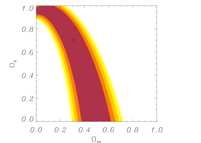
Figure 7: $\chi^{2}$ confidence levels in the $(\Omega_{m},\Omega_{\lambda})$ plane obtained from the optimisation of the lens configuration shown in Fig. 6. The 2 main cluster parameters $v_{c}$ and $\theta_{s}$ were recovered with $\chi^{2}_{\mathrm{min}}=0$. The cross (+) represents the original values $(\Omega_{m}^{0},\Omega_{\lambda}^{0})=(0.3,0.7)$. Dark to light colors delimit the confidence levels (from 1-$\sigma$ to 4-$\sigma$).

Figure 8: Solid lines: distribution of the best-fit velocity dispersion $v_{c}$ from the optimisation of the lens configuration shown in Fig. 6, for each cosmological model. The cross (+) represents the original value for $(\Omega_{m}^{0},\Omega_{\lambda}^{0})=(0.3,0.7)$: $v_{c}=2000$ km s^-1. Dashed lines correspond to the 1$\sigma$ confidence level contours from Fig. 7.

3.3.2 Changing the shape of the mass profile

To test the sensitivity of the method to the chosen fiducial mass profile, we tried to recover the lens with another potential, namely an elliptical HK profile, keeping the same simulated lens. $\sigma_{0}$, $\theta_{a}$ and $\theta_{s}$ were left free for the optimization. We first optimized the geometrical parameters for an arbitrary choice of cosmological parameters. The best values found are: $x_{0}=0.059\arcsec$, $y_{0}=0.063\arcsec$, $\theta=-0.063\degr$, and $\epsilon=0.280$. These values are close to the generating ones ($x_{0}=y_{0}=0\arcsec$, $\theta=0\degr$), except for the ellipticity which does not correspond to the same physical meaning in the pseudo-elliptical NFW profile (Golse & Kneib, 2002). They were then kept fixed for the rest of the optimization. For the lens parameters, we found $\sigma_{0}=1230^{+50}_{-50}$ km s^-1, $\theta_{a}=4.6\arcsec^{+0.2}_{-0.1}$ and $\theta_{s}=190\arcsec^{+20}_{-10}$. The confidence levels in the $(\Omega_{m},\Omega_{\lambda})$ plane are displayed in Fig. 9.

Although the reconstruction with a potential model different from the initial “real” one does not perfectly fit the data, the results are quite satisfactory. The confidence levels are even tighter than in the previous case, but the HK-type potential is characterised by one additional parameter or equivalently one degree of freedom less ($\nu=11$), compared to the pseudo-elliptical NFW profile. Nevertheless we find a minimum reduced $\chi^{2}=5$ rather far from 0.

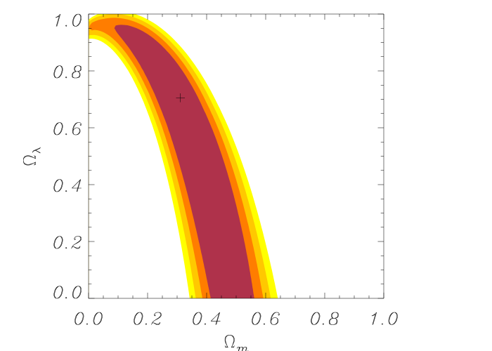
Figure 9: $\chi^{2}$ confidence levels in the $(\Omega_{m},\Omega_{\lambda})$ plane obtained from the optimisation of the lens configuration shown in Fig. 6. In this plot, the potential was fitted with a model different from the initial one (an elliptical HK profile instead of a pseudo-elliptical NFW). Dark to light colors delimit the confidence levels (from 1-$\sigma$ to 4-$\sigma$).

Several other mass profiles were tested as we wanted to discriminate between the different families of density profiles and test their sensitivity in the estimate of the cosmological parameters after the lens reconstruction. We used 5 types of profiles, namely:
i) the pseudo-elliptical NFW profile (Golse & Kneib, 2002),
ii) the singular isothermal ellipsoid (SIE) with $\rho(R)=\rho_{0}/R^{2}$, $R$ being the elliptical coordinate (Eq.(21)),
iii) the isothermal ellipsoid with core radius (CIE), obtained by replacing $R$ by $\sqrt{R^{2}+a^{2}}$ in the previous expression (see Kovner, 1989),
iv) the HK profile (Eq.(6)),
v) and the King profile characterised by

$$\rho(R)=\rho_{0}\ \frac{1+\frac{1-2\alpha}{3}\,R^{2}/a^{2}}{\left(1+R^{2}/a^{2}\right)^{2+\alpha}}.$$ (26)

The first 2 profiles are cusped, while the latter have a core radius and then an additional parameter. For each mass model, we generated the system of images defined in Table 2 (except for the SIE for which the radial system consists only of 2 images). We then fitted these images with the other 4 models. All the lens parameters were left free in this optimisation to get the minimum reduced $\chi^{2}$. We did not change the cosmological parameters in these recoveries. The results are presented in Table 3. We note that the “core-radius” profiles (especially the HK and King ones) can easlily recover the systems generated by any other models. Indeed in the fit of cusped lens images by shallower profiles, the core radius can be reduced to very small values to mimic a large density slope near the center. This is not the case for the cusped models which cannot mimic images given by a finite core radius lens model.

Table 3: Results of the lens reconstruction using a mass model different from the one used to generate the systems of images. The minimum reduced $\chi^{2}$ is given for each simulation.

Input profile	HK	King	CIE	NFW	SIE
Fitted profile
HK ($\nu=11$)	0.	23.	72.	460.	4500.
King ($\nu=11$)	33.	0.	33.	150.	1500.
CIE ($\nu=11$)	23.	0.26	0.	87.	2800.
NFW ($\nu=12$)	6.2	21.	18.	0.	680.
SIE ($\nu=12$)	0.14	0.011	0.28	76.	0.

3.3.3 Influence of the number of multiple systems

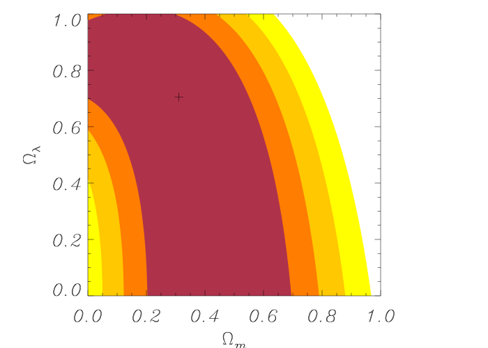
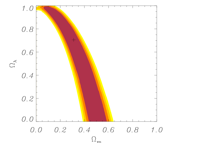
Figure 10: $\chi^{2}$ confidence levels in the $(\Omega_{m},\Omega_{\lambda})$ plane obtained from the optimisation of the lens configuration described in Table 5. Left: 2 systems and $\nu=10-4=6$ degrees of freedom. Middle: 3 systems and $\nu=16-5=11$ degrees of freedom. Right: 4 systems and $\nu=20-5=15$ degrees of freedom. The cross (+) represents the original values $(\Omega_{m}^{0},\Omega_{\lambda}^{0})=(0.3,0.7)$. Dark to light colors delimit the confidence levels (from 1-$\sigma$ to 4-$\sigma$).

In the preceding sections we considered 3 systems of multiple images. As the method proposed is based on the difference of angular distance ratios for different redshift planes, we now investigate the influence of the number of image families. The potential model is again an HK-type profile at $z_{\mathrm{L}}=0.3$ with $\sigma_{0}=1400$ km s^-1, $\theta_{a}=13.5$″(i.e. 65 kpc), $\theta_{s}=146$ ″(i.e. 700 kpc) and $\epsilon=0.2$. With 2 systems of images, we consider only 2 free parameters for the cluster, because there are not enough observables to yield results for more parameters, while in the other cases, 3 parameters are fitted. In all cases, these parameters are strongly constrained by the fit. Table 4 reports the errors on the fitted parameters in the optimisation process, for the different sets of multiple images detailed in Table 5. The differences in the fitted parameters between the different cases are small, as they are already well constrained with a single multiple images system.

Table 4: Recovering of the free parameters of the lens potential for the Table 5 different systems of images. The errors represent the variation of the fitted parameters at 1-$\sigma$ level when scanning the $(\Omega_{m},\Omega_{\lambda})$ plane in the optimisation process.

Nb of systems	$\sigma_{0}$ (km s-1)	$\theta_{a}$ (″)	$\theta_{s}$ (″)
2	$1400^{+60}_{-60}$	$13.5^{+0.25}_{-0.15}$	–
3	$1400^{+70}_{-60}$	$13.5^{+0.3}_{-0.2}$	$146^{+2}_{-2}$
4	$1400^{+60}_{-60}$	$13.5^{+0.3}_{-0.2}$	$146^{+14}_{-6}$

The expected constraints on $(\Omega_{m},\Omega_{\lambda})$ tighten when the number of families of multiple images increases (Fig. 10), especially when their redshift distribution is wide. 2 families would only provide marginal information on the cosmological parameters whereas 4 spectroscopically measured systems would give very tight error bars, provided they are well distributed in redshift.

Table 5: Sets of multiple images used in the simulations to test the influence of their number. $n_{i}$ represents the number of images used for each family. It does not include the central de-magnified image created for tangential images. $N_{C}$ is the number of constraints in the lens modeling for each family. $N_{C}=2\times n_{i}-2$.

Nb of systems	Family	Type	$n_{i}$	$z_{\mathrm{S}}$	$N_{C}$
2	$i=1$	Tangential	4	0.6	6
	$i=2$	Radial	3	1.	4
	$i=1$	Tangential	4	0.6	6
3	$i=2$	Radial	3	1.	4
	$i=3$	Tangential	4	2.	6
	$i=1$	Tangential	4	0.6	6
4	$i=2$	Radial	3	1.	4
	$i=3$	Tangential	4	2.	6
	$i=4$	Radial	3	4.	4

3.3.4 Influence of additional galaxy masses

In the previous parts, we considered only a main cluster potential with a regular morphology. We now test the contribution of individual galaxies, following the prescription used by Natarajan & Kneib (1996) as in Section 3.1. We generated 3 systems of multiple images formed by the sum of a main cluster with the mass density (HK-type) characterised by $\sigma_{0}=1400$ km s^-1, $\theta_{a}=13\arcsec$ and $\theta_{s}=150\arcsec$ and 12 individual galaxies which represent 30% of the total cluster mass (Fig. 11).

Figure 11: Multiple images generated by a cluster at $z_{\mathrm{L}}=0.3$ with an elliptical HK lens profile and the parameters: $\sigma_{0}=1400$ km/s, $\theta_{a}=13.54$″($a=65$ kpc) and $\theta_{s}=145.8$″($s=700$ kpc). 12 individual galaxies are added in the potential. 3 families of multiple images are identified (see Table 2 for details). We represent the radial (inside) and tangential (outside) critical lines corresponding to the multiple images redshifts. Their characteristic radii are increasing with redshift. Units are given in arcseconds.

The images were reconstructed using a main cluster potential with the same kind of shape as the initial one and the contribution of the galaxies scaled with $\sigma_{0}^{G}$. In addition, we fixed $\sigma_{0}^{G}$ proportional to $\sigma_{0}$ to avoid an increase of the number of free parameters. Consequently, any variation in $\sigma_{0}$ means a rescaling of the total mass of the cluster. So at first order we find that $\sigma_{0}^{2}\ E$ is constant when we scan the $(\Omega_{m},\Omega_{\lambda})$ plane. Keeping the geometrical parameters fixed ($x_{0}=y_{0}=0\arcsec$, $\theta=0\degr$, and $\epsilon=0.2$), we obtain the confidence levels in the $(\Omega_{m},\Omega_{\lambda})$ plane plotted in Fig. 12 and the following constraints on the potential parameters: $\sigma_{0}=1400^{+60}_{-65}$ km s^-1, $\theta_{a}=13\arcsec^{+0.3}_{-0.3}$ and $\theta_{s}=151\arcsec^{+1}_{-1}$.

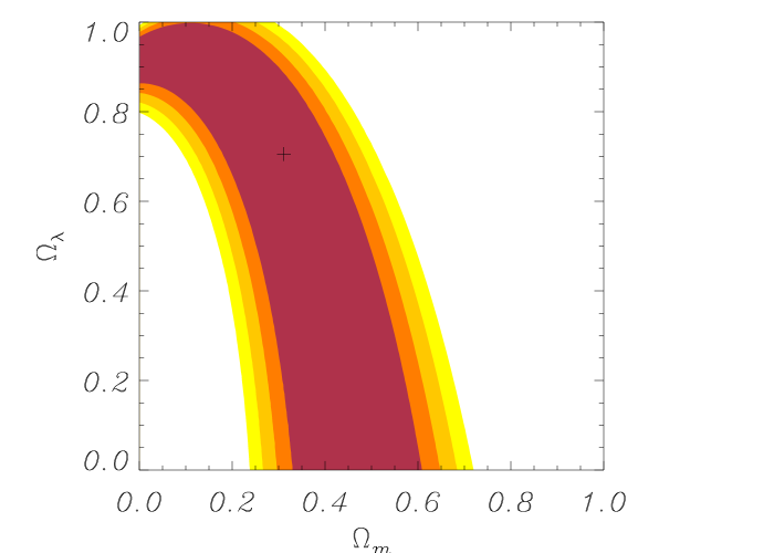
Figure 12: $\chi^{2}$ confidence levels in the $(\Omega_{m},\Omega_{\lambda})$ plane obtained from the optimisation of the lens configuration shown in Fig. 11. For the individual galaxies, we assumed that their mass is scaled with the total mass with $\sigma_{0}^{G}\propto\sigma_{0}$. The 3 main cluster parameters $\sigma_{0}$, $\theta_{a}$ and $\theta_{s}$ were recovered with $\chi^{2}_{\mathrm{min}}=0$ and $\nu=11$ degrees of freedom. Dark to light colors delimit the confidence levels (from 1-$\sigma$ to 4-$\sigma$).

To test the influence of the individual galaxies, we tried a reconstruction without their contribution. For the geometrical parameters first optimised we obtain $x_{0}=0.227\arcsec$, $y_{0}=0.060\arcsec$, $\theta=-0.748\degr$ and $\epsilon=0.193$, still close to the generating values. The confidence levels in the $(\Omega_{m},\Omega_{\lambda})$ plane are plotted in Fig. 13. The contours are slightly shifted and widened compared to the “good” ones (Fig. 12) but not significantly different. The minimum reduced $\chi^{2}$ is 17. So we are able to correctly retrieve the cluster potential, even without the individual galaxies ($\sigma_{0}=1380^{+70}_{-60}$ km s^-1, $\theta_{a}=11.9\arcsec^{+0.3}_{-0.2}$ and $\theta_{s}=180\arcsec^{+3}_{-3}$). Adding their contribution is nevertheless useful to determine precisely the minimum region and to tighten the confidence levels. It becomes quite critical in more complex cases or when a single galaxy strongly perturbs the location of an image.

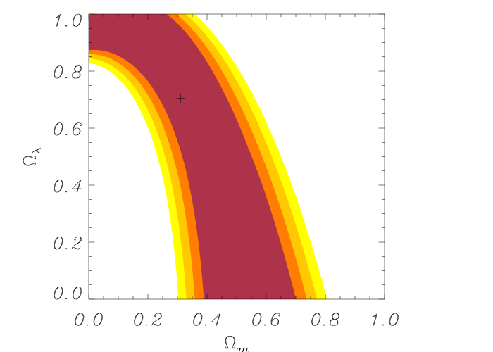
Figure 13: $\chi^{2}$ confidence levels in the $(\Omega_{m},\Omega_{\lambda})$ plane obtained from the optimisation of the lens configuration shown in Fig 11. Here, we did not introduce the individual galaxies when recovering the global potential. The 3 main cluster parameters $\sigma_{0}$, $\theta_{a}$ and $\theta_{s}$ were recovered but with a non-zero reduced $\chi^{2}_{\mathrm{min}}$ ($\chi^{2}_{\mathrm{min}}=17$). Dark to light colors delimit the confidence levels (from 1-$\sigma$ to 4-$\sigma$).

3.3.5 Bi-modal cluster mass distribution

Up to this point, we have considered simple clusters, dominated by a single massive component. In reality, most clusters are not fully virialised and present sub-structure as the result of accretion processes or merging phases. With these more complex mass distributions, the lensing configurations are more widely distributed. Therefore we examine how the cosmological parameters can be constrained with this type of realistic mass distribution. We thus generated a bi-modal cluster consisting of two clumps of equal mass and 3 families of multiple images probing each part of the lens (Fig. 14). The total potential is axisymmetric and each clump is characterised by an HK-type elliptical mass profile. As the number of multiple images is rather small, we limited the number of parameters to recover and chose $\sigma_{0}$ and $\theta_{a}$ for each clump as adjustable variables. Therefore we fixed $x_{01}=-34\arcsec$, $x_{02}=34\arcsec$, $y_{01}=y_{02}=0\arcsec$, $\theta_{1}=-45\degr$, $\theta_{2}=+45\degr$, $\epsilon_{1}=\epsilon_{2}=0.2$ and $\theta_{s1}=\theta_{s2}=167\arcsec$.

Figure 14: Multiple images generated by a bimodal cluster at $z_{\mathrm{L}}=0.3$ with the lens parameters: $\sigma_{01}=\sigma_{02}=1100$ km/s, $\theta_{a1}=\theta_{a}{2}=12\arcsec$ (58 kpc) and $\theta_{s1}=\theta_{s2}=167\arcsec$ (800 kpc). 3 families of multiple images are identified at $z_{S1}=0.7$, $z_{S2}=1$ and $z_{S3}=2$. Units are given in arcseconds.

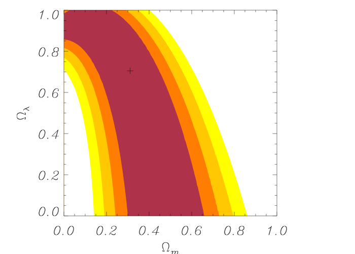
Figure 15: $\chi^{2}$ confidence levels in the $(\Omega_{m},\Omega_{\lambda})$ plane obtained from the optimisation of the lens configuration shown in Fig 14. The main cluster parameters $\sigma_{01}$, $\sigma_{02}$, $\theta_{a1}$ and $\theta_{a2}$ were recovered with $\chi^{2}_{\mathrm{min}}=0$ and a number of degrees of freedom $\nu=6$. The cross (+) represents the original values $(\Omega_{m}^{0},\Omega_{\lambda}^{0})=(0.3,0.7)$. Dark to light colors delimit the confidence levels (from 1-$\sigma$ to 4-$\sigma$).

Fixing again the initial values of $(\Omega_{m}^{0},\Omega_{\lambda}^{0})$ to the $\Lambda$CDM model $(0.3,0.7)$, we obtain the confidence levels plotted in Fig. 15. The contours are widened compared to the case of a single potential (in this case, the number of degrees of freedom is reduced from 11 to 6, but they still give reasonable constraints). Moreover we note that there is little variation in the fitted parameters: $\sigma_{01}=1100^{+55}_{-50}$ km s^-1, $\sigma_{02}=1100^{+55}_{-45}$ km s^-1, $\theta_{a1}=12.1\arcsec^{+0.1}_{-0.1}$, and $\theta_{a2}=12.1\arcsec^{+0.3}_{-0.2}$. This configuration is close to the case of the cluster Abell 370, modeled with a bi-modal mass distribution (Kneib et al., 1993b; Bézecourt et al., 1999b) needed to reproduce the peculiar shape of the central multiple-image system. Unfortunately, up to now only two redshifts are known for the multiple images identified in A370!

Figure 16: Multiple images generated by a cluster at $z_{\mathrm{L}}=0.3$ consisting of a main clump ($\sigma_{0}=1400$ km/s, $\theta_{a}=13.54\arcsec$ – 65 kpc – and $\theta_{s}=145.8\arcsec$ – 700 kpc) and a smaller one ($\sigma_{0}=500$ km/s, $\theta_{a}=5.2\arcsec$ – 25 kpc – and $\theta_{s}=45.9\arcsec$ – 220 kpc) located $102\arcsec$ from the main one. Close to their respective critical lines, 3 families of multiple images are identified: a tangential one (# 1, $z_{S1}=0.6$), a radial one (# 2, $z_{S2}=1$) and another tangential one (# 3, $z_{S3}=2$). Units are given in arcseconds.

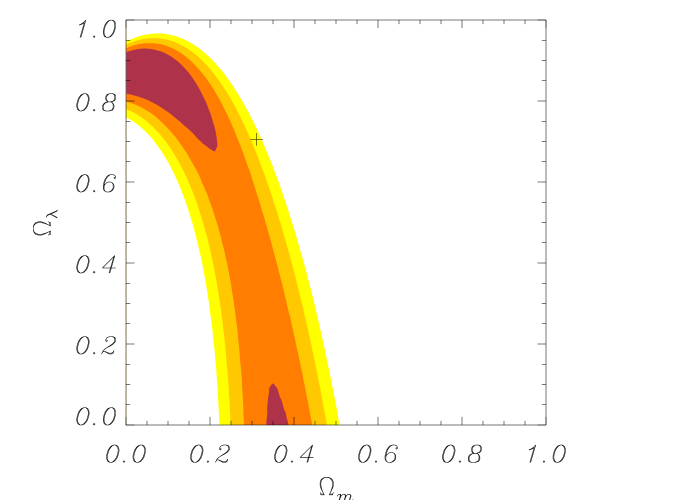
Figure 17: $\chi^{2}$ confidence levels in the $(\Omega_{m},\Omega_{\lambda})$ plane obtained from the optimisation of the lens configuration shown in Fig. 16. The 3 main cluster parameters $\sigma_{0}$, $\theta_{a}$ and $\theta_{s}$ were recovered with a reduced $\chi^{2}_{\mathrm{min}}=9$ and a number of degrees of freedom $\nu=11$. The cross (+) which represents the original values $(\Omega_{m}^{0},\Omega_{\lambda}^{0})=(0.3,0.7)$ is now outside the 3-$\sigma$ confidence levels. Dark to light colors delimit the confidence levels (from 1-$\sigma$ to 4-$\sigma$).

Last, we generated another system of 3 families of multiple images produced by a cluster consisting of a main clump ($\sigma_{0}=1400$ km s^-1) and a smaller one ($\sigma_{0}=500$ km s^-1) representing 22% of the total mass (Fig. 16). We chose to miss the small clump in the mass recovery as this may happen when dealing with some “dark clumps”. Fitting the configuration with a single main cluster, we found in a first round the geometrical parameters, which then remain constant in the $\chi^{2}$-optimisation: $x_{0}=0.348\arcsec$, $y_{0}=0.189\arcsec$, $\theta=1.880\degr$ and $\epsilon=0.259$. We note in particular that the ellipticity is larger than the one used to generate the main clump ($\epsilon=0.2$). This seems to be the response of the fitting process in order to mimic the missing second clump.

The parameters left free are again $\sigma_{0}$, $\theta_{a}$ and $\theta_{s}$. The confidence contours are shown in Fig. 17. We found the following values of the parameters: $\sigma_{0}=1400^{+40}_{-70}$ km s^-1, $\theta_{a}=12.8\arcsec^{+0.2}_{-0.2}$ and $\theta_{s}=169\arcsec^{+2}_{-2}$. However in this case, we do not recover correctly the set of cosmological parameters used to generate the system: $(\Omega_{m},\Omega_{\lambda})=(0.3,0.7)$ is excluded at the 3-$\sigma$ level. Moreover the shape of the contours is not the one expected from the lensing degeneracy. This could be considered to be a signature of an incorrect fiducial mass distribution due to a missing clump in the mass reconstruction. This example demonstrates that the initial guess and the modeling of the different components of a cluster are very sensitive elements. They need to be carefully determined if one wants to test further constraints on the cosmological parameters

4 Conclusion and future prospects

In this paper we have explored in detail a method to obtain informations on the geometry of the Universe with gravitational lensing. It follows an approach first presented by Link & Pierce (LP98) which states that multiple imaging systems at different redshifts can provide constraints not only on the mass profile of the lensing cluster but also on second order parameters like $\Omega_{m}$ or $\Omega_{\lambda}$ – contained in angular size distances ratios. We have shown that this technique gives constraints which are degenerate in the $(\Omega_{m},\Omega_{\lambda})$ plane and that the degeneracy is roughly perpendicular to the degeneracy issued from high-redshift supernovae searches. Moreover, the matter density $\Omega_{m}$ can be better constrained than the $\Lambda$-term. Several simulations of lensing configurations are proposed, assuming reasonable conditions on the cluster-lens potential, such as a regular morphology modeled with only a few parameters. Provided high quality data can be obtained on at least 3 systems of multiple images, such as high resolution images (HST-type) for accurate image positions and deep spectroscopic data for the measurement of the source redshifts, we can expect typical error bars of $\Omega_{m}=0.30{\pm 0.11}$, $\Omega_{\lambda}=0.70{\pm 0.23}$.

Table 6: List of 6 redshift configurations used in the combination of different cluster-lenses (Fig. 18) for a global $\chi^{2}$ minimisation.

$z_{\mathrm{L}}$	$z_{S1}$	$z_{S2}$	$z_{S3}$
0.15	0.4	0.8	2.0
0.2	0.5	1.0	3.0
0.25	0.6	0.9	2.0
0.3	0.6	1.0	2.0
0.35	0.6	1.5	3.0
0.4	0.8	1.8	4.0

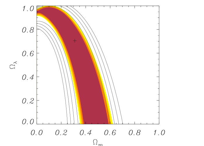
Figure 18: Color scale: $\chi^{2}(\Omega_{m},\Omega_{\lambda})$ confidence levels obtained for a combination of 6 different cluster-lenses configurations (see Table 6 for redshift informations). The 3 main cluster parameters $\sigma_{0}$, $\theta_{a}$, $\theta_{s}$ were recovered for each cluster with a reduced $\chi^{2}_{\mathrm{min}}=0$ and $\nu=60$ degrees of freedom. Dark to light colors delimit the confidence levels (from 1-$\sigma$ to 4-$\sigma$). Solid lines: $\chi^{2}$ confidence levels (from 1-$\sigma$ to 4-$\sigma$) obtained for a single cluster at $z_{\mathrm{L}}=0.3$ (same as Fig. 7). The cross (+) represents the original values $(\Omega_{m}^{0},\Omega_{\lambda}^{0})=(0.3,0.7)$.

It is important to underline that one cluster-lens with adequate multiple images would provide by itself a strong constraint on the geometry of the whole Universe. Such clusters are not that rare: MS2137.3–2353, MS0440.5+0204, A370, A1689, A2218, AC114 are certainly good candidates for such an experiment. A thorough and detailed analysis is still to be done and we have in hand most of the tools to address the problem immediately. Furthermore, as the exact degeneracy in the ($\Omega_{m}$ , $\Omega_{\lambda}$) plane depends only on the values of the different redshift planes involved, combining results from different cluster-lenses can tighten the error bars. For illustration, we combined 6 different lens configurations and source redshifts, as listed in Table 6. Compared to the expected results with a single cluster (solid lines), the constraints can be improved significantly (Fig. 18).

Looking for a good accuracy on the cosmological parameters is a permanent search in cosmology. Although the curvature is now determined with a remarkable precision thanks to recent results from CMB balloon experiments, it is still very difficult to disentangle $\Omega_{m}$ from $\Omega_{\lambda}$ (Zaldarriaga et al., 1997). Therefore the advantages of joint analyses by several independent approaches have been pointed out (see White (1998) and Efstathiou et al. (1999)): combined results from the $m-z$ relation for SNIa and CMB power spectrum analyses (which have orthogonal degeneracies) constrain $\Omega_{m}$ or $\Omega_{\lambda}$ separately with much higher accuracy than the individual experiments alone, leading to the currently favored model. One impressive example has been given by Hu & Tegmark (1999) who showed that a relatively small weak lensing survey could dramatically improve the accuracy of the cosmological parameters measured by future CMB missions.The combination of independent tests can improve the constraints as well as serve as a consistency check. This is clearly demonstrated by Helbig et al. (1999) who combine constraints from lensing statistics and distant SNIa to get a narrow range of possible values for $\Omega_{\lambda}$. Therefore, gravitational lensing is a powerful complementary method to address the determination of the geometrical cosmological parameters and probably one of the cheapest ones, compared to CMB experiments or SNIa searches. Our technique, when applied to about 10 clusters, should be included in such joint analysis, to obtain a consistent picture on the present cosmological parameters. We are truly entering an era of accurate cosmology, where the overlap between the allowed regions of parameter space is becoming quite reduced.