The SAURON project. I. The panoramic integral-field spectrograph

Abstract

A new integral-field spectrograph, SAURON, is described. It is based on the TIGER principle, and uses a lenslet array. SAURON has a large field of view and high throughput, and allows simultaneous sky subtraction. Its design is optimized for studies of the stellar kinematics, gas kinematics, and line-strength distributions of nearby early-type galaxies. The instrument design and specifications are described, as well as the extensive analysis software which was developed to obtain fully calibrated spectra, and the associated kinematic and line-strength measurements. A companion paper reports on the first results obtained with SAURON on the William Herschel Telescope.

1 Introduction

Determining the intrinsic shapes and internal dynamical and stellar population structure of elliptical galaxies and spiral bulges is a long-standing problem, whose solution is tied to understanding the processes of galaxy formation and evolution (Franx, Illingworth & de Zeeuw 1991; Bak & Statler 2000). Many galaxy components are not spherical or even axisymmetric, but triaxial: N-body simulations routinely produce triaxial dark halos (Barnes 1994; Weil & Hernquist 1996); giant ellipticals are known to be slowly-rotating triaxial structures (Binney 1976, 1978; Davies et al. 1983; Bender & Nieto 1990; de Zeeuw & Franx 1991); many bulges, including the one in the Galaxy, are triaxial (Stark 1977; Gerhard, Vietri & Kent 1989; Häfner et al. 2000); bars are strongly triaxial (Kent 1990; Merrifield & Kuijken 1995; Bureau & Freeman 1999). Key questions for scenarios of galaxy formation include: What is the distribution of intrinsic triaxial shapes? What is, at a given shape, the range in internal velocity distributions? What is the relation between the kinematics of stars (and gas) and the stellar populations? Answers to these questions require morphological, kinematical and stellar population studies of galaxies along the Hubble sequence, combined with comprehensive dynamical modeling.

The velocity fields and line-strength distributions of triaxial galaxy components can display a rich structure, that are difficult to map with traditional long-slit spectroscopy (Arnold et al. 1994; Statler 1991, 1994; de Zeeuw 1996). Furthermore, in many elliptical galaxies, the central region is ‘kinematically decoupled’: the inner and outer regions appear to rotate around different axes (e.g., Franx & Illingworth 1988; Bender 1988; de Zeeuw & Franx 1991; Surma & Bender 1995). This makes two-dimensional (integral-field) spectroscopy of stars and gas essential for deriving the dynamical structure of these systems and for understanding their formation and evolution.

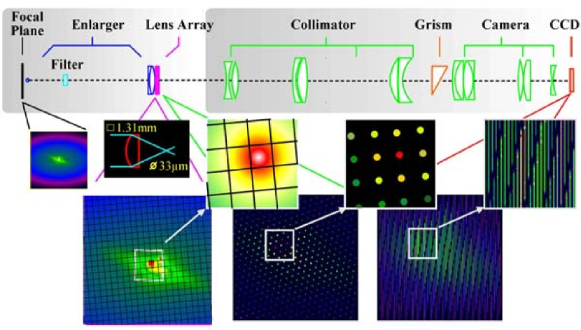
Figure 1: Optical layout of SAURON. The main optical elements are displayed from the telescope focal plane (left) to the detector plane (right). The image of a galaxy is shown successively at the telescope focal plane, at the entrance plane of the lens array, at the exit plane of the lens array and at the detector plane. A zoom-in of a small area of the galaxy is shown at each plane. The insert shows the detailed light path within a microlens.

In the past decade, substantial instrumental effort has gone into high-spatial resolution spectroscopy with slits (e.g., STIS on HST, Woodgate et al. 1998), or with integral-field spectrographs with small field of view (e.g., TIGER and OASIS on the CFHT; Bacon et al. 1995, 2000) to study galactic nuclei. By contrast, studies of the large-scale kinematics of galaxies still make do with long-slit spectroscopy along at most a few position angles (e.g., Davies & Birkinshaw 1988; Statler & Smecker-Hane 1999). While useful for probing the dark matter content at large radii (e.g., Carollo et al. 1995; Gerhard et al. 1998), long-slit spectroscopy provides insufficient spatial coverage to unravel the kinematics and line-strength distributions of early-type galaxies. Therefore, we decided to build SAURON (Spectroscopic Areal Unit for Research on Optical Nebulae), an integral-field spectrograph optimized for studies of the kinematics of gas and stars in galaxies, with high throughput and, most importantly, with a large field of view. We are using SAURON on the 4.2m William Herschel Telescope (WHT) on La Palma to measure the mean streaming velocity $V$, the velocity dispersion $\sigma$ and the velocity profile (or line-of-sight velocity distribution, LOSVD) of the stellar absorption lines and the emission lines of ionized gas, as well as the two-dimensional distribution of line-strengths and line-ratios, over the optical extent of a representative sample of nearby early-type galaxies. The first results of this project are described in Davies et al. (2001) and de Zeeuw et al. (2001, Paper II).

This paper presents SAURON, and is organized as follows: §2 describes the design, the choice of the instrumental parameters and the construction of the instrument; the results of commissioning and instrument calibration are reported in §3, and the extensive set of data reduction software we developed to calibrate and analyze SAURON exposures are detailed in §4 and §5; §6 presents a first result, and §7 sums up.

2 The SAURON spectrograph

The design of SAURON is similar to that of the prototype integral-field spectrograph TIGER, which operated on the CFHT between 1987 and 1996 (Bacon et al. 1995), and of OASIS, a common-user integral-field spectrograph for use with natural guide star adaptive optics at the CFHT (Bacon et al. 2000). Fig. 1 illustrates the optical layout: a filter selects a fixed wavelength range, after which an enlarger images the sky onto the heart of the instrument, a lenslet array. Each lenslet produces a micropupil, whose light, after a collimator, is dispersed by a grism. A camera then images the resulting spectra onto a CCD, aligned with the dispersion direction but slightly rotated with respect to the lenslet array to avoid overlap of adjacent spectra.

2.1 Setting instrumental parameters

Compared to OASIS, which is dedicated to high spatial resolution, a large field of view is the main driver of the SAURON design. There are a number of free parameters which can be used to maximize the field of view: the spectral length in CCD pixels, the perpendicular spacing between adjacent spectra (which we refer to as the cross-dispersion separation), the detector size and the lenslet size on the sky. The latter is related to the diameter of the telescope and the aperture of the camera for a given detector pixel size (see eq. [12] of Bacon et al. 1995). For the 4.2m aperture of the WHT and the 13.5 $\mu\mbox{m}$ pixels of the 2k$\times$4k EEV 12 detector this limits the lenslet size to a maximum of about $1^{\prime\prime}$ in order to keep the camera aperture slower than $f/1.8$.

Table 1: Current specification of SAURON on the WHT.

	HR mode	LR mode
Spatial sampling	$0\hbox{$.\!\!^{\prime\prime}$}27$	$0\hbox{$.\!\!^{\prime\prime}$}94$
Field of view	$9^{\prime\prime}\times 11^{\prime\prime}$	$33^{\prime\prime}\times 41^{\prime\prime}$
Spectral resolution (FWHM)	2.8 Å	3.6 Å
Instrumental dispersion ($\sigma_{\mathrm{inst}}$)	90 $\mbox{km~{}s}^{-1}$	105 $\mbox{km~{}s}^{-1}$
Spectral sampling	1.1 Å pix-1
Wavelength range	4500–7000 Å
Initial spectral window	4760–5400 Å
Calibration lamps	Ne, Ar, W
Detector	EEV 12 $2148\times 4200$
Pixel size	13.5 $\mu\mbox{m}$
Instrument Efficiency	35%
Total Efficiency	14.7%

The cross-dispersion separation is a critical parameter. Its value is the result of a compromise: on the one hand, it should be as small as possible in order to maximize the number of spectra on the detector; on the other hand, it should be large enough in order to avoid overlap of neighbouring spectra. For SAURON, the chosen value of 4.8 pixels gives up to 10% overlap between adjacent spectra (see Fig. 9). The trade-off for this small cross-dispersion separation was to invest significant effort in the development of specific software to account for this overlap at the stage of spectra extraction (see §4.2). Given the fast aperture of the camera, we decided to limit its field size by using only 2k$\times$3k pixels on the detector. The required image quality can then be obtained with a reasonable number of surfaces, so that the throughput is as high as possible.

The spectral length is the product of the spectral coverage and the spectral sampling. We selected the 4800–5400 Å range so as to allow simultaneous observation of the [Oiii] and H$\beta$ emission lines to probe the gas kinematics, and of a number of absorption features (the Mg$b$ band, various Fe lines and again H$\beta$) for measurement of the stellar kinematics (mean velocity, velocity dispersion and the full LOSVD) and line-strengths. The adopted spectral dispersion of SAURON in the standard mode (see below) is $\sigma_{\mathrm{inst}}\simeq 90$ $\mbox{km~{}s}^{-1}$(with a corresponding sampling of 1.1 Å pixel^-1), which is adequate to measure the LOSVD of the stellar spheroidal components of galaxies which have velocity dispersions $\mathrel{\hbox to0.0pt{\lower 3.0pt\hbox{$\sim$}\hss}\raise 2.0pt\hbox{$>$}}100$ $\mbox{km~{}s}^{-1}$.

The final result is a field of view of $41^{\prime\prime}\times 33^{\prime\prime}$, observed with a filling factor of 100%. Each lenslet has a square shape and samples a $0\hbox{$.\!\!^{\prime\prime}$}94\times 0\hbox{$.\!\!^{\prime\prime}$}94$ area on the sky in this low-resolution (LR) mode (Table 1). This undersamples the typical seeing at La Palma, but provides essentially all one can extract from the integrated light of a galaxy over a large field of view in a single pointing.

To take advantage of the best seeing conditions, SAURON contains a mechanism for switching to another enlarger, resulting in a $9^{\prime\prime}\times 11^{\prime\prime}$ field of view sampled at $0\hbox{$.\!\!^{\prime\prime}$}27\times 0\hbox{$.\!\!^{\prime\prime}$}27$ (Table 1). This high-resolution (HR) mode can be used in conditions of excellent seeing to study galactic nuclei with the highest spatial resolution achievable at La Palma without using adaptive optics.

As the objective is to map the kinematics and line-strengths out to about an effective radius for nearby early-type galaxies, it is necessary to have accurate sky subtraction. However, for most objects, the field of view is still not large enough to measure a clean sky spectrum on it. We therefore incorporated in SAURON the ability to acquire sky spectra simultaneously with the object spectra. This is achieved by means of an extra enlarger pointing to a patch of sky located $1\hbox{$.\mkern-4.0mu^{\prime}$}9$ away from the main field: the main enlarger images the science field of view on the center of the lens array, while the sky field of view is imaged off to one side; a combination of a mask and a baffle is used to prevent light pollution between the two fields. This gives 1431 object lenslets and 146 sky lenslets (Fig. 2).

Figure 2: The SAURON lenslet position on the CCD. Open squares: object lenses, solid squares: sky lenses. The scale is in pixels. The sky lenses have the same shape and size as the object lenses (i.e., 0$.\!\!^{\prime\prime}$94 in the LR mode and 0$.\!\!^{\prime\prime}$27 in the HR mode), but are shifted 1$.\mkern-4.0mu^{\prime}$9 away from the center of the field.

2.2 Design and realization

The SAURON optics were designed by Bernard Delabre (ESO). The main difficulty was to accommodate the required fast aperture of the camera ($f/1.8$). To maximize the throughput and stay within a limited budget, the optics were optimized for the range 4500–7000 Å, rather than for the whole CCD bandwidth (0.35–1 $\mu\mbox{m}$). This provides the required image quality (80% encircled energy within a 13 $\mu\mbox{m}$ radius) with a minimum number of surfaces and no aspheres. The required spectroscopic resolution is obtained with a 514 lines mm^-1 grism and a 190 mm focal-length camera.

The lens array (Fig. 3) is constructed from two arrays of cylindrical lenses mounted at right angles to each other. This assembly gives the geometrical equivalent of an array of square lenses of 1.31 mm on the side. Two identical enlargers—one for the object and the other for the sky—with a magnification of 6.2 are used in front of the lens array to produce the LR mode (0$.\!\!^{\prime\prime}$94 sampling). A similar pair of enlargers with a magnification of 22.2 provides the HR mode (0$.\!\!^{\prime\prime}$27 sampling). An interference filter with a square transmission profile selects the 4760–5400 Å wavelength range. The filter transmission is above 80% over more than 80% of this wavelength range. The filter is tilted to avoid ghost images and, as a consequence, the transmitted bandwidth moves within the field. As will be discussed in §4.9, this reduces the useful common bandwidth by 16%.

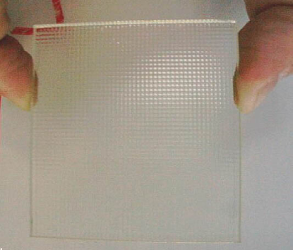
Figure 3: The SAURON lenslet array is made from two sets of cylindrical barrels of $1.31\times 70$ mm² in fused silica. It consists of over 1600 square lenslets, each of which is 1.31 mm on the side.

The mechanical design of SAURON is similar to that of OASIS: a double octapod mounted on a central plate which supports the main optical elements. This design is light and strong, and minimizes flexure (cf. §3). Fig. 4 shows the instrument mounted on the Cassegrain port of the WHT.

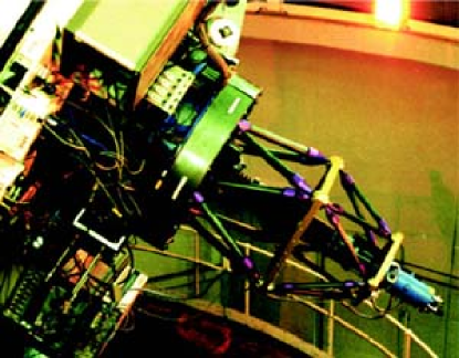
Figure 4: SAURON at the Cassegrain port of the WHT during the commissioning run in February 1999.

Because of its limited number of observing modes (LR/HR), SAURON has only three mechanisms: the focal plane wheel, for the calibration mirror, the enlarger wheel, which supports the two sets of twin enlargers, and a focusing mechanism for the camera. The latter has a linear precision and repeatibility of a few $\mu\mbox{m}$, which is required to ensure a correct focus at $f/1.8$. The temperature at the camera location is monitored during the night.

Calibration is performed internally using a tungsten lamp as continuum source, and neon and argon arc lamps as reference for wavelength calibration. Special care is taken in the calibration path to form an equivalent of the telescope pupil with the correct figure and location. This is particularly relevant for TIGER-type integral-field spectrographs, since pupils are imaged onto the detector.

All movements are controlled remotely with dedicated electronics. Commands are sent by a RS432 link from the control room, where a Linux PC is used to drive the instrument. A graphical user interface (GUI) written in Tcl/Tk allows every configuration changes to be made with ease.

3 Commissioning

SAURON was commissioned on the WHT in early February 1999. In the preceding days, the instrument, together with the control software, was checked and interfaced to the WHT environment. Particular attention was paid to the optical alignment between SAURON and the detector (dispersion direction along the CCD columns and $5.18^{\circ}$ rotation between dispersion direction and lenslet array). The most labour-intensive part was to adjust the CCD to be coplanar with the camera focal plane, so that there is no detectable systematic gradient in the measured point spread function (PSF). This must be done accurately since a small residual tilt would rapidly degrade the PSF within the illuminated area of the CCD. A specific procedure was developed to ease this part of the setup. The instrument performed very well from the moment of first light on February 1st (de Zeeuw et al. 2000).

Fig. 5 presents some typical SAURON exposures taken during commissioning. Panel a shows a small part of an exposure with the grism taken out, yielding an image of the micropupils. Panels b and c show spectra obtained with the internal tungsten and neon lamps, respectively. The former shows the accurately aligned continuum spectra, while the latter displays the emission lines used for wavelength calibration. Panel d presents spectra of the central region of NGC 3377 (see §6).

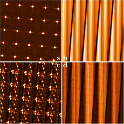
Figure 5: Examples of SAURON exposures taken during commissioning. Each panel shows only a small part of the entire CCD frame so that details can be seen. a) Micropupil image taken with the grism out. Each cross is the diffraction pattern from one square lenslet. b) Continuum image using the tungsten lamp. c) Neon arc. d) Central part of NGC 3377.

We measured flexure by means of calibration exposures taken at 1800 s interval while tracking, and found $0.2\pm 0.1$ pixels of shift between zenith and 1.4 airmasses. We also measured the total throughput of SAURON, including atmosphere, telescope and detector, using photometric standard stars observed on a number of photometric nights. The throughput response is flat at 14.7% (Fig. 6), except for a small oscillation caused by the intrinsic response of the filter. This is within a few percent of the value predicted by the optical design.

Figure 6: Total measured throughput of SAURON (including telescope, atmosphere and CCD transmission).

With this efficiency, a signal-to-noise S/N of about 25 per spatial and spectral element can be reached in 1800 s for a surface brightness $\mu_{V}\sim 19$ mag arcsec^-2 (Fig. 7). This corresponds to the typical surface brightness at radii of $\sim$$15^{\prime\prime}$ in early-type galaxies. By exposing for two hours and co-adding adjacent spectra in the lower surface brightness outer regions, we can achieve S/N $\mathrel{\hbox to0.0pt{\lower 3.0pt\hbox{$\sim$}\hss}\raise 2.0pt\hbox{$>$}}50$, as required for the derivation of the shape of the LOSVD (see e.g., van der Marel & Franx 1993).

Figure 7: Signal-to-noise ratio S/N (per pixel) of individual SAURON spectra as a function of surface brightness, for an integration time of 1800 s. The solid line indicates the LR mode and the dashed line is for HR mode.

4 Data Analysis

A typical SAURON exposure displays a complex pattern of 1577 individual spectra which are densely packed on the detector (see Fig. 5). This pattern defines a three-dimensional data-set $(\alpha,\delta,\lambda)$ (which we refer to as a data-cube), where $\alpha$ and $\delta$ are the sky coordinates of a given lenslet, and $\lambda$ is the wavelength coordinate. We developed a specific data reduction package for SAURON, with the aim of (i) producing a wavelength- and flux-calibrated data-cube from a set of raw CCD exposures, and (ii) extracting the required scientific quantities (e.g., velocity fields of stars and gas, line-strength maps, etc.) from the data-cubes, as well as providing tools to display them.

The software is based on the XOasis data reduction package (Bacon et al. 2000), which includes a library, a set of routines and a GUI interface. All core programs are written in C ($285\,000$ lines), while the GUI uses the Tcl/Tk toolkit ($34\,000$ lines). While some programs are common to both OASIS and SAURON, some instrument-dependent programs were developed specifically for SAURON, including those for the extraction of spectra (see also Copin 2000). The package is called XSauron, and is described below.

4.1 CCD preprocessing

The CCD preprocessing is standard, and includes overscan, bias and dark subtraction.

The overscan value of each line of a raw frame is computed using the average of 40 offset columns. A median filter of five lines is then applied to remove high frequency features. The result is subtracted line by line from the raw exposure. The master bias is then obtained by taking the median of a set of normalized biases.

Darks do not show any significant pattern after bias subtraction, thus a constant value can be removed from each frame. This equals the nominal value of EEV 12, 0.7 e^-1 pixel^-1 hour^-1. The dark current therefore plays a negligible role for our typical integration times of 1800 s.

The SAURON software formally includes the possibility to correct for pixel-to-pixel flat-field variations. As for the EEV 12, apart from a few cosmetic defects, the pixel-to-pixel variations observed from a flat-field continuum exposure are quite small (a few percent at most) and difficult to quantify in our case: it would require measuring the relative transmission of each pixel on the detector with very high signal to noise, but, as illustrated in Fig. 5, the detector is strongly non-uniformly illuminated, especially in the cross-dispersion direction. We therefore decided not to correct for pixel-to-pixel flat-field variations. As we will see below, the resulting error is smoothed out at the extraction stage, where we average adjacent columns.

The EEV 12 has two adjacent bad columns, one saturated and the other blind. We interpolate linearly over them. This simple interpolation scheme is not able to recover the correct intensity value of the spectra which straddle the bad columns. However, since the extraction process takes into account neighbouring spectra (see §4.2), it is necessary to remove saturated or zero pixel values to avoid contaminating adjacent spectra. The corresponding lenslet is then simply removed at a later stage (see §4.9).

4.2 Extraction of spectra

The extraction of the individual spectra from the raw CCD frame is the most instrument-specific part of the data reduction process. It is also the most difficult, because of the dense packing of the spectra on the detector (see Fig. 5). Fig. 9 illustrates that a simple average of a few columns around the spectrum peak position will fail to produce satisfactory results, since it would include light from the wings of neighbouring spectra. The fact that neighbouring spectra on the detector are also neighbours on the sky does not help due to the shift in wavelength (see right panel of Fig. 10). We must therefore accurately remove the contribution of neighbours when computing the spectral flux.

The method we developed is based on the experience gained with TIGER and OASIS, but with significant improvements to reach the accuracy required here. The principle is to fit an instrumental chromatic model to high signal-to-noise calibration frames. The resulting parameters of the fit are saved in a table called the extraction mask, which is then applied to every preprocessed frame to obtain the corresponding uncalibrated data-cube.

4.2.1 Building the extraction mask

Building the extraction mask requires three steps: (i) lenslet location measurement, (ii) cross-dispersion profile analysis and (iii) global fitting of the instrumental model.

A micropupil exposure (see Fig. 5a) is obtained with the tungsten lamp on and the grism removed. Except for the magnification and some geometrical distortion, this exposure is a direct image of the lenslet array, and is suitable for deriving its geometrical characteristics. Each small spot also provides a good measure of the overall instrumental PSF, i.e., the telescope geometric pupil convolved by the PSF of the spectrograph with the grism removed. There are other means to obtain this PSF, e.g., using the calibration frames, but the micropupils are easier to use since they are free of any contamination from neighbours, being separated by large distances (54 pixels, cf. the 4.8 pixel separation between adjacent spectra).

After automatic thresholding, the centroids of the micropupils are computed and the basic parameters of the lens array (lenslet positions and tilt with respect to the detector columns) are derived. The geometrical distortion of the spectrograph can be evaluated using the observed difference between the measured micropupil position and the theoretical one as a function of radius. In contrast to the case of OASIS, the geometrical distortion of SAURON is negligible over the detector area.

We now describe in more detail the model of the cross-dispersion profile and its variation over the field of view. For a good treatment of the pollution by neighbouring spectra (and optimal extraction), we are only interested in the profile of the PSF along the cross-dispersion direction, while the dispersion profile directly sets the spectral resolution of the observations. In order to be compatible with the observed cross-dispersion profile of a continuum spectrum, the PSF must be collapsed along the dispersion direction to obtain its integrated cross-dispersion profile (ICDP). For convenience, we make no formal distinction between the PSF and its ICDP.

The overall ICDP ${\cal P}$ is the convolution of the geometrical micropupil profile ${\cal G}$ with the PSF of the spectrograph ${\cal F}$. The former can be computed easily knowing the primary mirror and central obstruction size, the aperture of the lenslet on the sky, and the aperture of the camera. Accordingly, the micropupil geometrical size is 2.6 and 0.9 pixel for the LR and HR modes, respectively, and its ICDP—uniform over the CCD area—is shown in Fig. 8. For ease of computation, we represent the profile ${\cal G}$ by the sum of three Gaussian functions.

Figure 8: Integrated cross-dispersion profile ${\cal G}$ of the geometrical micropupil (solid line) and its fit (dashed line) with three Gaussian functions (dotted lines).

${\cal F}$, the second contribution to ${\cal P}$, is caused by imperfections in the lenslet array and spectrograph, and is likely to change with the instrument focus and setup, and to vary from one lenslet to the other. While the geometrical pupil is constant over the CCD area, the observed FWHM of the ICDP increases with distance from the optical center, and from red to blue on a given spectrum. We thus decided to model the spectrograph PSF ${\cal F}_{i}$ for lenslet $i$ as the convolution of a fixed part ${\cal F}^{\star}$ (the kernel) with a chromatic local component ${\cal F}_{i}(\lambda)$. Overall, the cross-dispersion profile ${\cal P}_{i}(\lambda)$ of spectrum $i$ at wavelength $\lambda$ is approximated by:

$${\cal P}={\cal G}\otimes{\cal F}^{\star}\otimes{\cal F}_{i}(\lambda).$$ (1)

Due to the absence of a dispersing element, ${\cal F}_{i}(\lambda)$ cannot be retrieved from the micropupils, but if we restrict our analysis to the micropupils very close to the optical center, where ${\cal F}_{i}(\lambda)$ is Dirac-like, ${\cal G}\otimes{\cal F}^{\star}$ can be derived. A sum of three centered Gaussians gives a precise approximation of the kernel. The corresponding fit, which takes into account the pixel integration, is performed simultaneously on the ten central micropupils. This procedure results in an accurate kernel shape without being affected by undersampling.

In the second step, the last component ${\cal F}_{i}(\lambda)$ of Eq. (1) must be derived from a spectroscopic exposure, using the previously estimated ${\cal G}\otimes{\cal F}^{\star}$ kernel. For this purpose, we use a high signal-to-noise continuum exposure obtained with the tungsten lamp (see Fig. 5b). A single Gaussian is enough to describe this component, but the dense packing requires the simultaneous fit of a group of cross-dispersion profiles, and makes the process CPU intensive. The fit is accurate to a few percent, as shown in Fig. 9. Given the slow variation of $\sigma_{{\cal F}_{i}}(\lambda)$ with $\lambda$, we perform this fit only once for each ten CCD lines. At each analysed line $y$, the position $x$ and width $\sigma$ of each peak is saved in a file for later use as input data for the global mask fitting.

Figure 9: Upper panel: example of a cross dispersion profile derived from a continuum exposure (thick solid line) and its fit by the model described in text (thin solid line). To illustrate the level of overlap, only the central three fitted profiles are shown (dashed lines). Lower panel: relative residual of the fit (in %).

The above construction of the ICDP produces a large collection of $(x,y,\sigma)$ giving position and characteristic width of all the cross-dispersion peaks over the entire detector. The final step is to link these unconnected data to individual spectra. By contrast to the two previous steps, which involve only local fitting, this last operation requires the fit of a global instrumental chromatic model, based on an a priori knowledge of basic optical parameters measured in the laboratory: the camera and collimator focal lengths, and the number of grooves of the grism. It also requires the fitting of extra parameters which depend on the setup of the instrument and/or were not previously measured with enough accuracy: (i) the three Euler angles of the grism, (ii) the chromatic dependence of the collimator and camera focal lengths, (iii) the distortion parameters of the collimator and camera optics as well as their chromatic dependence, and (iv) the distortion center of the optical system.

The fitting of the instrumental model requires the $(x,y,\sigma)$ measurements of the cross-dispersion profiles and an arc exposure with its corresponding emission-line wavelengths tabulated. The latter is needed to constrain efficiently the wavelength-dependent quantities. The fit uses a simple ray-tracing scheme, with ‘ideal’ optical components, to predict the $(x,y)$ location of each spectrum as function of wavelength $\lambda$. The predicted locations of the continuum spectra and the arc emission lines are compared with the corresponding data and differences are minimized by the fit (Fig. 10). Convergence is obtained after a few hundred iterations with a simplex scheme. The model is then accurate to $\mathrel{\hbox to0.0pt{\lower 3.0pt\hbox{$\sim$}\hss}\raise 2.0pt\hbox{$<$}}0.1$ pixel RMS.

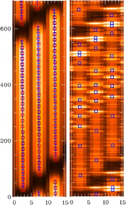
Figure 10: Example of mask-fitting results. Left panel: a small part of a continuum exposure with the derived locations of the spectra (crosses) and the corresponding fitted values (squares). Right panel: the corresponding arc (Neon) exposure and fitted emission lines (squares). The images have been expanded along the cross-dispersion axis for clarity.

The ICDP has a noticeable chromatic variation, causing a $\sim$$15$% relative increase of its width from the red (5400 Å) to the blue end (4760 Å). The slope of this chromatic variation is fit with a linear relation for each individual spectrum. The last improvement is to allow for tiny offsets and rotations of the spectra which are not included in our simple mathematical model of the instrument, in order to get the most precise mask position.

The final mask describes the best model of the instrument, including second-order lens-to-lens adjustments. This mask is accurate for a full run, and has been computed precisely for the first run. The setup can vary slightly from run to run, but most of the optical parameters (e.g., the focal length) are stable. We therefore adopt a simplified procedure using the mask from the first run as starting point, and fitting only the parameters that are likely to change with the setup, such as the global translation and rotation of the detector.

4.2.2 Extracting spectra

The preparatory work described in the above has only one objective: to extract accurate spectro-photometric spectra from the preprocessed CCD frames. The procedure requires (i) the lenslet position in sky coordinates, (ii) the location of the spectra in CCD coordinates and the corresponding wavelength coordinates, and (iii) the ICDP of the spectra. All this information is stored in the instrumental model contained in the extraction mask. However, before the extraction process itself, we must take into account possible small displacements of the positions of the spectra relative to the extraction mask. These offsets are due to a small amount of mechanical flexure between the mask exposure—generally obtained at zenith—and the object exposure. They are estimated using the cross-correlation function between arc exposures obtained before and/or after the object exposure and the arc exposure used for the mask creation.

For each lenslet $i$ referenced in the extraction mask, the instrumental model gives the $(x_{i},y_{i},\lambda(y_{i}))$ geometrical position on the CCD of the corresponding spectrum. At each position, one must compute the total flux which belongs to the associated spectrum (see Fig. 9). This step is critical, as any error will affect the spectro-photometric accuracy of the extracted spectrum. We developed an algorithm to remove the pollution induced by the two neighbouring spectra and to compute the flux in an optimal way (as defined by Horne 1986 and Robertson 1986). The algorithm uses the ICDP of the three adjacent peaks (the current spectrum and its two neighbours). The three profiles are normalized to the intensity of the peaks, and the estimated cross-dispersion profile of the neighbours is subtracted from the main peak in a dual-pass procedure. Finally, the total flux of the main peak is calculated in an extraction window of five pixels width, using a weighted sum of the intensity of the pixels, corrected for the pollution by neighbours. The total variance of the integrated flux is saved as an estimate of the spectrum variance.

Examples of this process are shown in Fig. 11, which is repeated along each pixel of the current spectrum. The result is saved in a specific binary structure called the TIGER data-cube. This contains all the extracted intensity spectra and their corresponding variance spectra. Each pair of object & noise spectra is referenced by a lens number. The data-cube is attached to a FITS table containing the corresponding lens coordinates and any other pertinent data.

Figure 11: Examples of flux computation in the extraction process on continuum (upper panel) and neon arc (lower panel) exposures. Thick solid line: data. Thin solid line: sum of the estimated central-plus-neighbours cross-dispersion profiles. Dashed lines: individual cross-dispersion profiles.

4.3 Wavelength calibration

The wavelength calibration is standard, and uses neon arc exposures which contain 11 useful emission lines in the SAURON wavelength range. Since the extraction process is based on a chromatic model, the raw extracted spectra are already pre-calibrated in wavelength (scale $\lambda^{\prime}$). Therefore, the final wavelength calibration only needs to correct for second order effects which were not included in the instrumental model, and is thus straightforward and robust. A cubic polynomial is fitted to the $(\lambda^{\prime}_{k},\lambda_{k})$ points, and is saved for rebinning of the spectra. The RMS residual after rebinning is $\mathrel{\hbox to0.0pt{\lower 3.0pt\hbox{$\sim$}\hss}\raise 2.0pt\hbox{$<$}}0.1$ Å, which corresponds to 0.1 pixel or $\sim 5$ $\mbox{km~{}s}^{-1}$.

4.4 Flat-fielding

The flat-field is a complicated function of spatial coordinates $(x,y)$ and wavelength $\lambda$, which depends on the lenslet, filter, optics and detector properties. A continuum exposure obtained with the internal tungsten lamp gives featureless spectra, which can be used to remove the wavelength signature of the flat-field. However, the internal calibration illumination is not spatially uniform and cannot be used to correct for the spatial variation of the flat-field. For this, we use a twilight exposure. The final flat-field data-cube is the product of the spectral flat-field (obtained by dividing a reference continuum by the continuum data-cube) and the spatial flat-field variations measured on the twilight data-cube.

The flat-field correction displays a large-scale gradient from the upper to the lower regions of the detector, with a maximum of 20% variation over the whole field of view. At both edges of the filter, the very strong gradient of transmission is difficult to correct for, so we truncate each spectrum at the wavelength where the derivative of the transmission increases above a chosen threshold.

4.5 Cosmic ray removal

In imaging and long-slit spectroscopy, cosmic rays are generally removed directly from the CCD frame. The standard procedures are much more difficult to apply in the case of TIGER-type integral-field spectroscopy, since the high contrast arising from the organization of spectra on the detector prevents the use of standard algorithms. However, we can exploit the three-dimensional nature of the data-cube $(x,y,\lambda)$ to our advantage: using a continuity criterion in both the spatial and the spectral dimension on a wavelength-calibrated data-cube, we can detect any event which is statistically improbable. In practice, each spectrum is subtracted from the median of itself and its eight nearest spatial neighbours. The resulting spectrum, which corresponds to spatially unresolved structures, is filtered along the wavelength direction with a high-pass median filter. Statistically deviant pixels are then flagged as ‘cosmic rays’ and replaced by the values in the spatially medianed spectrum. The affected pixels are flagged also on the corresponding noise spectrum.

4.6 Uniform spectral resolution

At this stage, the spectra may have slightly different spectral resolutions over the field of view, due to, e.g., optical distorsions in the outer regions, CCD-chip flatness defects, non-orthogonality between CCD-chip mean plane and optical axis. In the SAURON LR mode, the instrumental spectral dispersion $\sigma_{\mathrm{inst}}$ typically increases from $\sim 90$ $\mbox{km~{}s}^{-1}$ close to the center to $\sim 110$ $\mbox{km~{}s}^{-1}$ at the edge of the field. We need to correct for this variation before we can combine multiple exposures of the same object obtained at different locations on the detector. For each instrumental setup, we derive the local instrumental spectral resolution over the field of view from the auto-correlation peak of a twilight spectrum. The spectral resolution of the data-cubes are then smoothed to the lower resolution using a simple Gaussian convolution.

4.7 Sky subtraction

Sky subtraction is straightforward: we simply compute the median of the 146 dedicated sky spectra and subtract it from the 1431 object spectra. The accuracy of sky subtraction, measured from blank sky exposures, is 5%. We also checked that the sky emission-line doublet [NI] $\lambda$5200 Å is removed properly.

4.8 Flux calibration

Flux calibration is classically achieved using spectro-photometric standard stars observed during the run as references. These stars are often dwarfs whose spectra generally exhibit few absorption features, although most of them show strong Balmer lines. The available tabulated flux curves usually have poor spectral resolution (sampling at a few tens of Å). Furthermore, systematic wavelength calibration errors of up to 6 Å at 5000 Å are not uncommon. This prevents an accurate flux calibration of the SAURON spectra which cover only a short wavelength region.

We therefore decided to favor flux-calibrated Lick (K0III) standards, previously observed at high spectral resolution, as SAURON flux-standard stars. These high-resolution stellar spectra are first convolved to the SAURON resolution and corrected to zero (heliocentric) velocity shift (using the Solar spectrum as a reference). The spectra are then used in place of the classical standard flux tables. This procedure provides an accuracy of about 5%.

Alternatively the relative transmission curve can also be measured using special stars with featureless spectra in the SAURON wavelength range. The derived curve is then scaled to absolute flux using photometric standard stars.

4.9 Merging multiple exposures

The total integration time on a galaxy is usually split into 1800 s segments. This value was chosen to limit the number of cosmic ray events and to avoid degradation of the spectral resolution caused by instrumental flexure (see §3). Another reason to split the integration in at least two exposures is to introduce a small spatial offset between successive exposures. These offsets are typically a few arcsec and correspond to a few spatial sampling elements. The fact that the same region of the galaxy is imaged on different lenslets is used in the merging process to minimise any remaining systematic errors, such as flat-field residuals, and to deal with a column of slightly lower quality lenslets. Furthermore, when a galaxy is larger than the SAURON field of view, it is also necessary to mosaic exposures of different fields, and the merging process has to build the global data-cube for the larger field from the individual data-cubes.

The merging process consists of four successive steps: (i) truncation of the spectra to a common wavelength range, (ii) relative centering of all individual data-cubes, (iii) computation of normalisation and weight factors, and (iv) merging and mosaicing of all data-cubes.

The spectral range varies over the field due to the tilt of the filter (see §2). The spectral range common to all spectra in the SAURON field is only 4825–5275 Å (Fig. 6). In some cases, a larger spectral coverage is required, which we can reach by ignoring some lenses, i.e., by shrinking the field. For instance, a wavelength range of 4825–5320 Å implies a reduction of the field of view by 36%.

After truncating all spectra to a common wavelength domain, we build integrated images for each individual data-cube by summing the entire flux in each spectrum and interpolating the resulting values. These reconstructed images are then centered using a cross-correlation scheme, taking care that the result is not affected by differences in seeing.

In principle, one should take into account the effects of differential atmospheric refraction before reconstructing images. By contrast to long-slit spectroscopy, here it is possible to correct for this effect if the integration time is short enough. The method is described in Arribas et al. (1999), and was applied successfully to TIGER and OASIS data (e.g., Emsellem at al. 1996). The galaxies in our representative sample will be observed at an airmass less than 1.3 (Paper II), so that the differential atmospheric refraction is sufficiently small (0$.\!\!^{\prime\prime}$16) to be neglected.

To optimize the use of telescope time, we do not observe photometric standards after each galaxy exposure. Changing observing conditions may cause normalisation errors in the flux calibration. We therefore renormalise all individual data-cubes using the common spatial area. During the merging process, each data-cube is also weighted to maximise the signal-to-noise ratio by an optimal summation scheme.

Finally, each data-cube is interpolated onto a common square grid. Since the different exposures are dithered by small spatial offsets, we use a finer grid to improve the spatial sampling of the combined data-cube (‘drizzling’ technique). At each grid point, the spectrum of the resulting merged data-cube is simply the weighted mean of all spectra available at this location. The variance of the merged spectra are derived from the variances of the individual spectra.

4.10 Palantir pipeline

The representative sample of galaxies that we are observing with SAURON (see Paper II) will generate an estimated total of 40 Gb of raw CCD frames and 20 Gb of reduced images and data-cubes. Some of the algorithms presented in the previous sections will evolve in time, to take into account the improved understanding of the instrument that comes with repeated use. In order to ease the re-processing of data-sets, we have developed a special pipeline environment, called Palantir. The main components of this are the SAURON software described above, a MySQL database, a Tcl/Tk interface for querying the database and sending data to the pipeline, and the OPUS pipeline management system (Rose et al. 1995). The database contains header information for the raw data, processing parameters and the log of data reduction. Using the interface, the desired class of data can be quickly selected and processed with the correct calibration files. OPUS was developed at STScI for managing the HST pipeline and provides tools for monitoring data in a pipeline. The extraction procedure is time consuming, so it is important to maximize the efficiency and the automation: OPUS does this by allowing parallel processing, on multiple CPUs if necessary.

The output of Palantir is one data-cube for each observed object with the instrumental signature removed. Each data-cube includes also a noise variance estimate. These ‘final’ data-cubes are the starting point for the scientific measurements. Below we summarize the main procedures we employ; more details will be found in subsequent papers that will address specific scientific questions, as the procedures sometimes need to be tailored to be able to deal with particular objects (e.g., counter-rotating disks).

5 Data analysis software

For scientific analysis, we need to measure a few key parameters from each spectrum of the final data-cube. These numbers, which could be, e.g., a flux, a velocity, or a line ratio, are attached to the spatial location of the corresponding spectrum. We then build two-dimensional images of these quantities, giving, e.g., velocity fields, line-strength maps, using a bilinear (or bicubic) interpolation scheme. The XSauron software allows us to display these images and examine the spectrum at a certain location interactively.

5.1 Photometry

A simple integration over the full wavelength range of the flux calibrated SAURON datacubes gives the reconstructed image of the target. This image gives the reference location of each spectrum. The kinematic and line-strength maps are by definition perfectly matched to this continuum intensity map. The reconstructed image can be used also to perform a photometric analysis of the object. In most cases this is not very useful since HST and/or ground-based broad-band images with finer sampling and a larger field of view will be available. However, a comparison of a high-resolution direct image with the SAURON reconstructed image provides an excellent test of the scientific quality of the instrument and the reduction algorithms. Any errors in the end-to-end process such as flat-field inaccuracies, or data extraction errors, will affect the reconstructed image and will be apparent in the comparison.

We have carried out a photometric comparison for the E3 galaxy NGC 4365, observed with SAURON in March 2000 (Davies et al. 2001). We used the GALPHOT package (Franx, Illingworth & Heckman 1989) to fit ellipses to the reconstructed image, and derive the standard photometric profiles. The same process was repeated on a high resolution image obtained from the HST/WFPC2 archive (#5454 PI Franx and #5920 PI Brache). We used the F555W filter since it is close to the SAURON bandpass. The HST image was convolved with a Gaussian of 2$.\!\!^{\prime\prime}$1 which is a rough estimate of the SAURON spatial resolution. The comparison is shown in Fig. 12. The SAURON data was normalized to the total flux of the HST image. The profiles agree very well: the RMS difference, excluding the central $2^{\prime\prime}$ (to avoid including any residual difference in spatial resolution) is only 0.016 in magnitude, 0.012 in ellipticity, and 1.0^∘ in position angle of the major axis.

Figure 12: A comparison of two photometric analyses of NGC 4365. The first (solid line) was obtained using ellipse fitting on HST/WFPC2 F555W data convolved with a 2$.\!\!^{\prime\prime}$1 PSF. The second (open circles) was derived in the same way from the SAURON reconstructed flux image in the 4850–5230 Å wavelength range. Top to bottom show profiles of surface brightness in magnitudes ($\mu_{v}$), $\Delta\mu=\mu_{\rm SAURON}-\mu_{\rm HST}$, ellipticity ($\epsilon$) and position angle of the major axis (PA).

5.2 Stellar kinematics

Stellar kinematical quantities are derived with a version of the Fourier Correlation Quotient (FCQ) algorithm of Bender (1990), implemented in the XSauron software. Other algorithms, including Fourier Fitting (van der Marel & Franx 1993) and Unresolved Gaussian Decomposition (Kuijken & Merrifield 1993) will be incorporated in the near future.

During an observing run, we obtain a set of stellar exposures with SAURON, e.g., G, K and M giants, which are fully reduced providing a corresponding set of stellar data-cubes. For each data-cube, we measure FWHM_⋆, the full-width-at-half-maximum of the PSF of the reconstructed stellar image. All spectra within 1 FWHM_⋆ of the brightest spectrum in the data-cube are summed, resulting in a single high-S/N stellar spectrum. All spectra—galaxy and stellar templates—are then rebinned in $\ln\lambda$, to have a scale proportional to velocity. A data-cube containing the LOSVDs of the galaxy is then derived via FCQ using a single stellar template, typically a K0 giant). We then measure the mean velocity $V$ and velocity dispersion $\sigma$ from the LOSVDs, and these values are used to build a linear combination of all observed stellar templates, the so-called ‘optimal stellar template’, which matches best the galaxy spectra. This optimal template is derived by a linear fit in real $\lambda$-space, and include a low-order polynomial continuum correction when needed. The LOSVDs are then rederived with the optimal template. We finally reconstruct maps of $V$ and $\sigma$ as well as the Gauss-Hermite moments $h_{3}$ and $h_{4}$ (see van der Marel & Franx 1993; Gerhard 1993) by measuring these values on the final LOSVD data-cube.

5.3 Gas kinematics

The construction of an optimal template, as described in §5.2, can be done individually for each spectrum in a galaxy data-cube, resulting in a corresponding ‘optimal template’ data-cube. If the presence of emission lines is suspected, contaminated wavelength regions can be masked easily during the template-fitting process in $\lambda$-space. The broadened optimal template spectra are then subtracted from the galaxy spectra yielding a data-cube (presumably) free of any contribution from the stellar component. Emission lines, if present, are then easily measurable, and their fluxes, velocities and FWHM can be derived, assuming, e.g., a Gaussian shape for each line. We then build the corresponding maps of the gaseous distribution, kinematics, as well as line ratios (e.g., H$\beta$/[Oiii]). In some cases, emission lines will be strong enough to perturb the derivation of the stellar LOSVDs. When this happens, we subtract the fitted emission lines from the original galaxy spectra, and then recompute (a third time, see §5.2) the LOSVDs and their corresponding velocity moments.

5.4 Line-strengths

Line-strength indices are measured in the Lick/IDS system (Worthey 1994). The wavelength range of the current SAURON setup allows measurements of the H$\beta$, Fe 5015, Mg$b$ and Fe 5270 indices. In order to transform our system of line-strengths onto the standard Lick system, we broaden each flux calibrated spectrum in the final data-cube to the Lick resolution of 8.4 Å (FWHM) (Worthey & Ottaviani 1997) and then measure the indices. All index measurements are then corrected for internal velocity broadening of the galaxies (e.g., Kuntschner 2000) using an ‘optimal stellar template’ and the velocity dispersion derived from each individual spectrum (see § 5.1).

Due to differences in the continuum shape between our data and the original Lick setup, there remain generally some small systematic offsets for some indices. In order to monitor these, we observe a number ($>10$) of Lick standard stars in each run, and compare our measurements with the Lick data (Trager et al. 1998). This ensures inter-run consistency and also allows us to remove the systematic offsets.

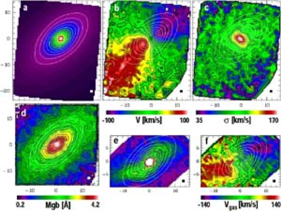
Figure 13: SAURON observations of the E6 galaxy NGC 3377. a) Reconstructed total intensity. b) Mean velocity $V$. c) Velocity dispersion $\sigma$. d) Stellar Mg$b$ index. e) Gaseous total intensity ([Oiii] $\lambda$5007). f) Gas velocity field. Isophotes of the reconstructed image are superimposed on each frame. The small square at the lower right corner of each frame gives the size of the lenslets ($0\hbox{$.\!\!^{\prime\prime}$}94\times 0\hbox{$.\!\!^{\prime\prime}$}94$), and the field shown is $30^{\prime\prime}\times 39^{\prime\prime}$. These maps are based on a $4\times 1800$ s exposure. No spatial binning has been applied at this stage. The stars show a striking rotating disk pattern with the spin axis misaligned about $10^{\circ}$ from the photometric minor axis, indicating the galaxy is triaxial. The gas also reveals strong non-axisymmetric structures and motions. The Mg$b$ isophotes follow the continuum light.

6 SAURON observations of NGC3377

The companion paper (Paper II) describes the first results of a systematic survey of nearby early-type galaxies with SAURON. Here, we illustrate the power and versatility of SAURON by presenting observations of the galaxy NGC 3377. This E6 galaxy in the Leo I group has a steep central luminosity profile (Faber et al. 1997), a total absolute magnitude $M_{B}=-19.24$, and has been probed for the kinematic signature of a massive central black hole from the ground (Kormendy et al. 1998).

We observed NGC 3377 with SAURON on February 17 1999, under photometric conditions, at a median seeing of 1$.\!\!^{\prime\prime}$5 (see Copin 2000). We exposed for a total of $4\times 1800$ s. Fig. 13 shows the resulting maps. The velocity field shows a regular pattern of rotation, but the rotation axis is misaligned by about $10^{\circ}$ from the photometric minor axis. This is the signature of a triaxial intrinsic shape. The Mbg isocontours seem to follow the continuum isophotes, but not the contours of constant dispersion. The ionised gas distribution and kinematics show strong departures from axisymmetry, this component exhibiting a spiral like morphology. This could be another manifestation of the triaxiality already probed via the stellar kinematics, and may be the signature of a bar-like system. This would not be too surprising since we expect anyway about two third of S0 galaxies to be (weakly or strongly) barred. This suggest that early-type systems with steep central luminosity profiles are not necessary axisymmetric. In this respect, it will be interesting to establish the mass of the central black hole.

The full analysis of the SAURON data for NGC 3377 will be presented elsewhere (Copin et al., in prep); it will include dynamical modeling which also incorporates OASIS observations of the central $2^{\prime\prime}\times 4^{\prime\prime}$ with a spatial resolution of 0$.\!\!^{\prime\prime}$6.

7 Concluding remarks

The number of integral-field spectrographs operating on 4–8 m class telescopes is increasing rapidly, and others are under construction or planned, including SINFONI for the VLT (Mengel et al. 2000) and IFMOS for the NGST (Le Fèvre et al. 2000). Much emphasis is being put on achieving the highest spatial resolution, by combining the ground-based spectrographs with adaptive optics, in order to be able to study e.g., galactic nuclei. SAURON was designed from the start to complement these instruments, for the specific purpose of providing the wide-field internal kinematics and line-strength distributions of nearby galaxies.

The plan to develop SAURON was formulated in the summer of 1995 and work commenced in late spring 1996. The instrument was completed in January 1999. This fast schedule was possible because SAURON is a special-purpose instrument with few modes, and because much use could be made of the expertise developed at Observatoire de Lyon through the building of TIGER and OASIS. While SAURON was constructed as a private instrument, plans are being developed to make it accessible to a wider community.

SAURON’s large field of view with 100% spatial coverage is unique, and will remain so for at least a few years. For comparison, INTEGRAL, which also operates on the WHT (Arribas et al. 1998), uses fibers and has a wider spectral coverage than SAURON. It has a mode with a $34^{\prime\prime}\times 29^{\prime\prime}$ field of view and $2\hbox{$.\!\!^{\prime\prime}$}7$ sampling, but the spatial coverage is incomplete and the throughput is relatively modest. VIMOS (on the VLT in 2001, see Le Fèvre et al. 1998) will have an integral-field spectrograph with spectral resolution relevant for galaxy kinematics and with a $27^{\prime\prime}\times 27^{\prime\prime}$ field sampled with $0\hbox{$.\!\!^{\prime\prime}$}67\times 0\hbox{$.\!\!^{\prime\prime}$}67$ pixels. The mode with a $54^{\prime\prime}\times 54^{\prime\prime}$ field of view has insufficient spectral resolution. SAURON’s $33^{\prime\prime}\times 41^{\prime\prime}$ field, together with its high throughput, make it the ideal instrument for studying the rich internal structure of nearby early-type galaxies.

It is a pleasure to thank the ING staff, in particular Rene Rutten and Tom Gregory, as well as Didier Boudon and Rene Godon for enthusiastic and competent support on La Palma. The very efficient SAURON optics were designed by Bernard Delabre and the software development benefitted from advice by Emmanuel and Arlette Pécontal. RLD gratefully acknowledges the award of a Research Fellowship from the Leverhulme Trust. The SAURON project is made possible through grants 614.13.003 and 781.74.203 from ASTRON/NWO and financial contributions from the Institut National des Sciences de l’Univers, the Université Claude Bernard Lyon I, the universities of Durham and Leiden, and PPARC grant ‘Extragalactic Astronomy & Cosmology at Durham 1998-2002’.

References

- [1] Arnold R.A., de Zeeuw P.T., Hunter C., 1994, MNRAS, 271, 924
- [2] Arribas S., Carter D., Cavaller L., del Burgo C., Edwards R., Fuentes F. J., Garcia A. A., Herreros J. M., Jones L. R., Mediavilla E., Pi M., Pollacco D., Rasilla J. L., Rees P. C., Sosa N. A., 1998, SPIE, 3355, 821
- [3] Arribas S., Mediavilla E., Garcia-Lorenzo B., del Burgo C., Fuensalida J.J., 1999, A&AS, 136, 189
- [4] Bacon R., Adam G., Baranne A., Courtes G., Dubet D., Dubois J.P., Emsellem E., Ferruit P., Georgelin Y., Monnet G., Pecontal E., Rousset A., Say F., 1995, A&AS, 113, 347
- [5] Bacon R., Emsellem E., Copin Y., Monnet G., 2000, in Imaging the Universe in Three Dimensions, eds W. van Breugel & J. Bland-Hawthorn, ASP Conf. Ser. 195, 173
- [6] Bak J., Statler T.S., 2000, AJ, 120, 110
- [7] Barnes J., 1994, in The Formation of Galaxies, Proc. Fifth Canary Winterschool of Astrophysics, eds C. Munoz-Tunon & F. Sanchez (Cambridge University Press), 399
- [8] Bender R., 1988, A&A, 202, L5
- [9] Bender R., 1990, A&A, 229, 441
- [10] Bender R., Nieto J.L., 1990, A&A, 239, 97
- [11] Binney J.J., 1976, MNRAS, 177, 19
- [12] Binney J.J., 1978, Comments Astrophys., 8, 27
- [13] Bureau M., Freeman K.C., 1999, AJ, 118, 126
- [14] Carollo C.M., de Zeeuw P.T., van der Marel R.P., Danziger I.J., Qian E.E., 1995, ApJ, 441, L25
- [15] Copin Y., 2000, PhD Thesis, ENS Lyon
- [16] Davies R.L., Birkinshaw M., 1988, ApJS, 68, 409
- [17] Davies R.L., Efstathiou G.P., Fall S.M., Illingworth G.D., Schechter P.L., 1983, ApJ, 266, 41
- [18] Davies R.L., Kuntschner H., Emsellem E., Bacon R., Bureau M., Carollo C.M., Copin Y., Miller B.W., Monnet G., Peletier R.F., Verolme E.K., de Zeeuw P.T., 2001, ApJL, in press
- [19] Emsellem E., Bacon R., Monnet G., Poulain P., 1996, A&A, 312, 777
- [20] Faber S. M., Tremaine S., Ajhar E. A., Byun Y. -I., Dressler A., Gebhardt K., Grillmair C., Kormendy J., Lauer T. R., Richstone D., 1997, AJ, 114, 1771
- [21] Franx M., Illingworth G.D., 1988, ApJ, 327, L55
- [22] Franx M., Illingworth G.D., Heckman T., 1989, AJ, 98, 538
- [23] Franx M., Illingworth G.D., de Zeeuw P.T., 1991, ApJ, 383, 112
- [24] Gerhard O.E., 1993, MNRAS, 265, 213
- [25] Gerhard O.E., Vietri M., Kent S.M., 1989, ApJ, 345, L33
- [26] Gerhard O.E., Jeske G., Saglia R.P., Bender R., 1998, MNRAS, 295, 197
- [27] Häfner R., Evans N.W., Dehnen W., Binney J.J., 2000, MNRAS, 314, 433
- [28] Horne K., 1986, PASP, 98, 609
- [29] Kent S.M., 1990, AJ, 100, 377
- [30] Kormendy J., Bender R., Evans A.S., Richstone D.O., 1998, AJ, 115, 1823
- [31] Kuijken K., Merrifield M.R., 1993, MNRAS, 264, 712
- [32] Kuntschner H., 2000, MNRAS, 315, 184
- [33] Le Fèvre O., Vettolani G.P., Maccagni D., Mancini D., Picat J.P., Mellier Y., Mazure A., Saisse M., Cuby J.G., Delabre B., Garilli B., Hill L., Prieto E., Arnold L., Conconi P., Cascone E., Mattaini E., Voet C., 1998, SPIE, 3355, 8
- [34] Le Fèvre O., Allington-Smith J., Prieto E., Bacon R., Content R., Cristiani S., Davies R.L., Delabre B., Ellis R.S., Monnet G., Pécontal E., Posselt W., Thatte N., de Zeeuw P.T., van der Werf P., 2000, in Imaging the Universe in Three Dimensions, eds W. van Breugel & J. Bland-Hawthorn, ASP Conf. Ser. 195, 431.
- [35] van der Marel R.P., Franx M., 1993, ApJ, 407, 525
- [36] Mengel S., Eisenhauer F., Tezca M., Thatte N., Röhrle C., Bickert K., Schreiber J., 2000, SPIE, 4005, 301
- [37] Merrifield M.R., Kuijken K., 1995, MNRAS, 274, 933
- [38] Robertson J.G., 1986, PASP, 98, 1220
- [39] Rose J., Akella R., Binegar S., Choo T.H., Heller-Boyer C., Hester T., Hyde P., Perrine R., Rose M.A., Steuerman K., 1995, ADASS, 4, 429
- [40] Stark A.A., 1977, ApJ, 213, 368
- [41] Statler T.S., 1991, ApJ, 382, L11
- [42] Statler T.S., 1994, ApJ, 425, 458
- [43] Statler T.S., Smecker-Hane T., 1999, AJ, 117, 839
- [44] Surma P., Bender R., 1995, A&A, 298, 405
- [45] Trager S.C., Worthey G., Faber S.M., Burstein D., Gonzalez J.J., 1998, ApJS, 116, 1
- [46] Weil M., Hernquist L., 1996, ApJ 460, 101
- [47] Woodgate B.E., et al., 1998, PASP, 110, 1183
- [48] Worthey G., Ottaviani D.L., 1997, ApJS, 111, 377
- [49] Worthey G., 1994, ApJS, 95, 107
- [50] de Zeeuw P.T., Franx M., 1991, ARA&A, 29, 239
- [51] de Zeeuw P.T., 1996, in Gravitational Dynamics, eds O. Lahav, E. Terlevich & R.J. Terlevich (Cambridge Univ. Press), 1
- [52] de Zeeuw P.T., Allington-Smith J.R., Bacon R., Bureau M., Carollo C.M., Copin Y., Davies R.L., Emsellem E., Kuntschner H., Miller B.W., Monnet G., Peletier R.F., Verolme E.K., 2000, ING Newsletter, 2, 11
- [53] de Zeeuw P.T., Bureau M., Emsellem E., Bacon R., Carollo C.M., Copin Y., Davies R.L., Kuntschner H., Miller B.W., Monnet G., Peletier R.F., Verolme E.K., 2001, MNRAS, submitted (Paper II).