Abstract

The results of analytical approximations and extensive calculations based on a path integral Monte Carlo (PIMC) scheme are presented. A new (direct) PIMC method allows for a correct determination of thermodynamic properties such as energy and equation of state of dense degenerate Coulomb systems. In this paper, we present results for dense partially ionized hydrogen at intermediate and high temperature. We give a quantitative comparison with the available results of alternative (restricted) PIMC simulations and with analytical expressions based on iterpolation formulas meeting the exact limits at low and high densities. Good agreement between the two simulations is found up to densities of the order of $10^{24}cm^{-3}$. The agreement with the analytical results is satisfactory up to densities in the range $10^{22}\dots 10^{23}cm^{-3}$.

1 Introduction

Correlated Fermi systems are of increasing interest in many fields, including plasmas, astrophysics, solids and nuclear matter, (see Kraeft et al. [1986]) for an overview. Among the topics of current interest are Fermi liquids, metallic hydrogen (see DaSilva et al. [1997]), plasma phase transition (see Schlanges et al. [1995]), bound states etc. In such many particle quantum systems, the Coulomb interaction is essential. There has been significant progress in recent years to study these systems theoretically, and especially numerically, (see e.g. Bonitz (Ed.) [2000], Zamalin et al. [1977], Filinov, A. V. et al. [2000]). A theoretical framework which is particularly well suited to describe thermodynamic properties in the region of strong coupling and degeneracy is the path integral quantum Monte Carlo (PIMC) method. There has been remarkable recent progress in applying these techniques to Fermi systems. However, these simulations are essentially hampered by the fermion sign problem. To overcome this difficulty, several strategies have been developed to simulate macroscopic Coulomb systems (see Militzer and Pollock [2000], Militzer and Ceperley [2000], and Militzer [2000]): the first is the restricted PIMC concept where additional assumptions on the density operator ${\hat{\rho}}$ are introduced which reduce the sum over permutations to even (positive) contributions only. This requires the knowledge of the nodes of the density matrix which is available only in a few special cases. However, for interacting macroscopic systems, these nodes are known only approximately, (see, e.g., Militzer and Pollock [2000] and Militzer and Ceperley [2000]), and the accuracy of the results is difficult to assess from within this scheme.

Recently, we have published a new path integral representation for the N-particle density operator (see Filinov, V. S., et al. [2000], Bonitz (Ed.) [2000], Filinov, V. S., et al. [2001]), which allows for direct Fermionic path integral Monte Carlo simulations of dense plasmas in a broad range of densities and temperatures. Using this concept we computed the pressure (equation of state, EOS), the energy, and the pair distribution functions of a dense partially ionized and dissociated electron–proten plasma (see Filinov, V. S., et al. [2000]). In this region no reliable data are available from other theories such as density functional theory or quantum statistics (see, e.g., Kraeft et al. [1986]), which would allow for an unambiguous test. Therefore, it is of high interest to perform quantitative comparisons of analytical results and independent numerical simulations, such as restricted and direct fermionic PIMC, which is the aim of this paper.

2 Path integral representation of thermodynamic quantities

We now briefly outline the idea of our direct PIMC scheme. All thermodynamic properties of a two-component plasma are defined by the partition function $Z$ which, for the case of $N_{e}$ electrons and $N_{p}$ protons, is given by

$$Z(N_{e},N_{p},V,\beta) = \frac{Q(N_{e},N_{p},\beta)}{N_{e}!N_{p}!},$$

$$\mbox{with}\qquad Q(N_{e},N_{p},\beta) = \sum_{\sigma}\int\limits_{V}dq\,dr\,\rho(q,r,\sigma;\beta),$$ (1)

where $\beta=1/k_{B}T$. The exact density matrix is, for a quantum system, in general, not known but can be constructed using a path integral representation (see Feynman and Hibbs [1965]),

$$\int\limits_{V}dR^{(0)}\sum_{\sigma}\rho(R^{(0)},\sigma;\beta) = \int\limits_{V}dR^{(0)}\dots dR^{(n)}\,\rho^{(1)}\cdot\rho^{(2)}\,\dots\rho^{(n)}$$ (2)

$$\times \sum_{\sigma}\sum_{P}(\pm 1)^{\kappa_{P}}\,{\cal S}(\sigma,{\hat{P}}\sigma^{\prime})\,{\hat{P}}\rho^{(n+1)},$$

where $\rho^{(i)}\equiv\rho\left(R^{(i-1)},R^{(i)};\Delta\beta\right)\equiv\langle R^{(i-1)}|e^{-\Delta\beta{\hat{H}}}|R^{(i)}\rangle$, whereas $\Delta\beta\equiv\beta/(n+1)$. ${\hat{H}}$ is the Hamilton operator, ${\hat{H}}={\hat{K}}+{\hat{U}}_{c}$, containing kinetic and potential energy contributions with ${\hat{U}}_{c}={\hat{U}}_{c}^{p}+{\hat{U}}_{c}^{e}+{\hat{U}}_{c}^{ep}$ being the sum of the Coulomb potentials between protons (p), electrons (e) and electrons and protons (ep). Further, $R^{(i)}=(q^{(i)},r^{(i)})\equiv(R_{p}^{(i)},R_{e}^{(i)})$, for $i=1,\dots n+1$, $R^{(0)}\equiv(q,r)\equiv(R_{p}^{(0)},R_{e}^{(0)})$. Also, $R^{(n+1)}\equiv R^{(0)}$ and $\sigma^{\prime}=\sigma$, i.e., the particles are represented by closed Fermionic loops with the coordinates (beads) $[R]\equiv[R^{(0)};R^{(1)};\dots;R^{(n)};R^{(n+1)}]$, where $r$ and $q$ denote the electron and proton coordinates, respectively. The spin gives rise to the spin part of the density matrix ${\cal S}$, whereas exchange effects are accounted for by the permutation operator ${\hat{P}}$, which acts on the electron coordinates and spin, and the sum over the permutations with parity $\kappa_{P}$. In the fermionic case (minus sign), the sum contains $N_{e}!/2$ positive and negative terms leading to the notorious sign problem. Due to the large mass difference of electrons and protons, the exchange of the latter is not included.

Recently, we have derived a new representation for the high–temperature density matrices $\rho^{(i)}$ in eq.(2) (see Filinov, V. S., et al. [2000]) which is well suited for direct PIMC simulations. A crucial point is that the electron–proton interaction can be described by an (effective) quantum pair potential $\Phi^{ep}$ (Kelbg–potential, see Kelbg [1964]). For details of the derivation see Filinov, V. S., et al. [2000]. Here, we present only the final result for the energy and for the EOS. Consider first the energy:

$$\beta E=\frac{3}{2}(N_{e}+N_{p})+\frac{1}{Q}\frac{1}{\,\lambda_{p}^{3N_{p}}\Delta\lambda_{e}^{3N_{e}}}\sum_{s=0}^{N_{e}}\int dq\,dr\,d\xi\,\rho_{s}(q,[r],\beta)\,\times$$

$$\Bigg{\{}\sum_{p<t}^{N_{p}}\frac{\beta e^{2}}{|q_{pt}|}+\sum_{l=0}^{n}\Bigg{[}\sum_{p<t}^{N_{e}}\frac{\Delta\beta e^{2}}{|r^{l}_{pt}|}+\sum_{p=1}^{N_{p}}\sum_{t=1}^{N_{e}}\Psi_{l}^{ep}\Bigg{]}$$

$$+\sum_{l=1}^{n}\Bigg{[}-\sum_{p<t}^{N_{e}}C^{l}_{pt}\frac{\Delta\beta e^{2}}{|r^{l}_{pt}|^{2}}+\sum_{p=1}^{N_{p}}\sum_{t=1}^{N_{e}}D^{l}_{pt}\frac{\partial\Delta\beta\Phi^{ep}}{\partial|x^{l}_{pt}|}\Bigg{]}$$

$$\,-\,\frac{1}{{\rm det}|\psi^{n,1}_{ab}|_{s}}\frac{\partial{\rm\,det}|\psi^{n,1}_{ab}|_{s}}{\partial\beta}\Bigg{\}},$$

$${\rm with}\quad C^{l}_{pt}=\frac{\langle r^{l}_{pt}|y^{l}_{pt}\rangle}{2|r^{l}_{pt}|},\qquad D^{l}_{pt}=\frac{\langle x^{l}_{pt}|y^{l}_{p}\rangle}{2|x^{l}_{pt}|},\quad$$ (3)

and $\Psi_{l}^{ep}\equiv\Delta\beta\partial[\beta^{\prime}\Phi^{ep}(|x^{l}_{pt}|,\beta^{\prime})]/\partial\beta^{\prime}|_{\beta^{\prime}=\Delta\beta}$ contains the electron-proton Kelbg potential $\Phi^{ep}$. Here, $\langle\dots|\dots\rangle$ denotes the scalar product, and $q_{pt}$, $r_{pt}$ and $x_{pt}$ are differences of two coordinate vectors: $q_{pt}\equiv q_{p}-q_{t}$, $r_{pt}\equiv r_{p}-r_{t}$, $x_{pt}\equiv r_{p}-q_{t}$, $r^{l}_{pt}=r_{pt}+y_{pt}^{l}$, $x^{l}_{pt}\equiv x_{pt}+y^{l}_{p}$ and $y^{l}_{pt}\equiv y^{l}_{p}-y^{l}_{t}$, with $y_{a}^{n}=\Delta\lambda_{e}\sum_{k=1}^{n}\xi^{(k)}_{a}$ and $\Delta\lambda_{a}^{2}=2\pi\hbar^{2}\Delta\beta/m_{a}$. We introduced dimensionless distances between neighboring vertices on the loop, $\xi^{(1)},\dots\xi^{(n)}$, thus, explicitly, $[r]\equiv[r;y_{e}^{(1)};y_{e}^{(2)};\dots]$.

The density matrix $\rho_{s}$ is given by

$$\rho_{s}(q,[r],\beta)=C^{s}_{N_{e}}\,e^{-\beta U(q,[r],\beta)}\prod\limits_{l=1}^{n}\prod\limits_{p=1}^{N_{e}}\phi^{l}_{pp}{\rm det}\,|\psi^{n,1}_{ab}|_{s},$$ (4)

where $U(q,[r],\beta)=U_{c}^{p}(q)+\{U^{e}([r],\Delta\beta)+U^{ep}(q,[r],\Delta\beta)\}/(n+1)$ and $\phi^{l}_{pp}\equiv\exp[-\pi|\xi^{(l)}_{p}|^{2}]$. We underline that the density matrix (4) does not contain an explicit sum over the permutations and thus no sum of terms with alternating sign. Instead, the whole exchange problem is contained in a single exchange matrix given by

$$||\psi^{n,1}_{ab}||_{s}\equiv||e^{-\frac{\pi}{\Delta\lambda_{e}^{2}}\left|(r_{a}-r_{b})+y_{a}^{n}\right|^{2}}||_{s}.$$ (5)

As a result of the spin summation, the matrix carries a subscript $s$ denoting the number of electrons having the same spin projection. For more detail, (see Filinov, V. S., et al. [2000], Bonitz (Ed.) [2000]). In a similar way, we obtain the result for the equation of state,

$$\frac{\beta pV}{N_{e}+N_{p}}=1+\frac{1}{N_{e}+N_{p}}\frac{(3Q)^{-1}}{\,\lambda_{p}^{3N_{p}}\Delta\lambda_{e}^{3N_{e}}}\sum_{s=0}^{N_{e}}\int dq\,dr\,d\xi\,\rho_{s}(q,[r],\beta)\times$$

$$\Bigg{\{}\sum_{p<t}^{N_{p}}\frac{\beta e^{2}}{|q_{pt}|}+\sum_{p<t}^{N_{e}}\frac{\Delta\beta e^{2}}{|r_{pt}|}-\sum_{p=1}^{N_{p}}\sum_{t=1}^{N_{e}}|x_{pt}|\frac{\partial\Delta\beta\Phi^{ep}}{\partial|x_{pt}|}$$

$$+\sum_{l=1}^{n}\left[\sum_{p<t}^{N_{e}}A^{l}_{pt}\frac{\Delta\beta e^{2}}{|r^{l}_{pt}|^{2}}-\sum_{p=1}^{N_{p}}\sum_{t=1}^{N_{e}}B^{l}_{pt}\frac{\partial\Delta\beta\Phi^{ep}}{\partial|x^{l}_{pt}|}\right]$$

$$\,+\,\frac{\alpha}{{\rm det}|\psi^{n,1}_{ab}|_{s}}\frac{\partial{\rm\,det}|\psi^{n,1}_{ab}|_{s}}{\partial\alpha}\Bigg{\}},$$

$${\rm with}\quad A^{l}_{pt}=\frac{\langle r^{l}_{pt}|r_{pt}\rangle}{|r^{l}_{pt}|},\qquad B^{l}_{pt}=\frac{\langle x^{l}_{pt}|x_{pt}\rangle}{|x^{l}_{pt}|}.\quad$$ (6)

3 Analytical approximations for the thermodynamic functions of dense plasmas

To describe dense plasmas, it is necessary to have thermodynamic functions valid at arbitrary degeneracy. Here, we restrict ourselves to the Hartree–Fock (HF) and the Montroll–Ward (MW) contributions. This approximation is appropriate at temperatures high enough such that the Coulomb interaction is weak and the possibility of the formation of bound states is excluded. HF and MW contributions have been computed numerically (see Kraeft et al. [1986]). The analytical evaluation of the MW contribution is possible in limiting situations only, namely in the low and very high density cases. In the intermediate region Padé formulae can be used to interpolate between the limiting cases. In between, the formulae are fitted to numerical data; (see Ebeling et al. [1981] , Haronska et al. [1987] and Ebeling and Richert [1985]). We give the excess free energy and the interaction part of the chemical potential of the electron gas,

$$f^{P}=\frac{f_{D}-\frac{1}{4}(\pi\beta)^{-1/2}{\bar{n}}+8{\bar{n}}^{2}f_{GB}}{1+8ln\left[1+\frac{3}{64\sqrt{2}}(\pi\beta)^{1/4}{\bar{n}}^{1/2}\right]+8{\bar{n}}^{2}}\,,$$ (7)

and

$$\mu^{P}=\frac{\mu_{D}-\frac{1}{2}(\pi\beta)^{-1/2}{\bar{n}}+8{\bar{n}}^{2}\mu_{GB}}{1+8ln\left[1+\frac{1}{16\sqrt{2}}(\pi\beta)^{1/4}{\bar{n}}^{1/2}\right]+8{\bar{n}}^{2}}\,.$$ (8)

In (7,8) Heaviside units $\hbar=\frac{e^{2}}{2}=2m_{e}=1$ and the dimensionless density ${\bar{n}}=n\Lambda^{3}$ were used.

Figure 1: Energy and pressure isotherms for $50,000K$ (solid line). Solid line with circles– Hartree Fock (HF) and Montroll–Ward (MW) approximation. Reference data: triangle – RPIMC (see Militzer et al.), square – DPIMC.

In formulae (7,8), the correct low density behaviour (Debye limiting law) is guaranteed by choosing $f_{D}=-(2/3)(\pi\beta)^{-1/4}{\bar{n}}^{1/2}$ and $\mu_{D}=-(\pi\beta)^{-1/4}{\bar{n}}^{1/2}\,.$ The correct high degeneracy limit is recovered by using the (slightly modified) Gell-Mann Brueckner approximations (including Hartree–Fock) for the free energy and for the chemical potential

$$f_{GB}=-\frac{0.9163}{r_{s}}-0.08883{\rm ln}\left[1+\frac{4.9262}{r_{s}^{0.7}}\right]\approx-\frac{0.9163}{r_{s}}+0.0622{\rm ln}r_{s}\,,$$ (9)

$$\mu_{GB}=-\frac{1.2217}{r_{s}}-0.08883{\rm ln}\left[1+\frac{6.2208}{r_{s}^{0.7}}\right]\approx-\frac{1.2217}{r_{s}}+0.0622{\rm ln}r_{s}\,.$$ (10)

The free energy is now equal to the internal energy at $T=0$ and reads, according to Carr and Maradudin,

$$\frac{U}{N}=\frac{2.21}{r_{s}^{2}}-\frac{0.916}{r_{s}}+0.0622{\rm ln}r_{s}-0.096+0.018r_{s}{\rm ln}r_{s}+\cdots\,.$$

The Brueckner parameter $r_{s}$ is given by $r_{s}^{3}=3/(4\pi n)$. While the Hartree Fock term, i.e., the $1/r_{s}$ term in (9,10), was retained unaffected, the additional terms in these equations and in formulae (7,8) were modified, or fitted, respectively, such that (7,8) meet the numerical data in between, where the analytical limiting formulae are not applicable.

Figure 2: Energy and pressure isotherms for $100,000K$ (solid line with circles). Solid line with small squares – Hartree Fock (HF) and Montroll–Ward (MW) approximation. Reference data: triangle – RPIMC (see Militzer et al. [2000]), large square – DPIMC.

Consider now the proton contributions. In the low density regime, the proton formulae are practically the same as for the electrons, whereas in the high density limit we adjust the formulae to (classical) Monte–Carlo (MC) data. We have for the free energy density and for the chemical potential

$$-\frac{f_{p}}{k_{B}Tn_{p}}=\frac{(-f_{p}^{\rm int}/k_{B}Tn_{p})_{D}[1-a{\tilde{n}}_{p}^{2/3}(f_{p}^{\rm int}/k_{B}Tn_{p})_{MC}]}{1-a{\tilde{n}}_{p}^{1/2}[{\tilde{n}}_{p}^{1/2}/(\frac{f_{p}^{\rm int}}{k_{B}Tn_{P}})_{D}+{\tilde{n}}_{p}^{1/6}(\frac{f_{p}^{\rm int}}{k_{B}Tn_{p}})_{D}]}\,$$ (11)

$$-\frac{\mu_{p}}{k_{B}T}=\frac{(-\mu_{p}^{\rm int}/k_{B}T)_{D}[1-2a{\tilde{n}}_{p}^{2/3}(\mu_{p}^{\rm int}/k_{B}Tn_{p})_{MC}]}{1-2a{\tilde{n}}_{p}^{1/2}[{\tilde{n}}_{p}^{1/2}/(\frac{\mu_{p}^{\rm int}}{k_{B}T})_{D}+{\tilde{n}}_{p}^{1/6}(\frac{\mu_{p}^{\rm int}}{k_{B}T})_{D}]}\,.$$ (12)

We used the abbreviation $a$ which depends only on temperature

$$a=\sqrt{\pi^{3}k_{B}T}\Big{\{}\frac{1}{2}\Big{[}1+\sqrt{\frac{k_{B}T}{4\pi}}{\rm exp}\Big{(}\frac{\sqrt{\pi}/2}{{\rm ln}{(4/k_{B}T)^{1/6}}-2\sqrt{k_{B}T}}\Big{)}\Big{]}-0.29931\Big{\}}\,.$$ (13)

For the protons, we introduce the dimensionless density to be used in the plasma parameter $\Gamma$, namely ${\tilde{n}}_{p}=\frac{8}{(k_{B}T)^{3}}n_{p}$, $\Gamma=\Big{(}\frac{4}{3}\pi{\tilde{n}}_{p}\Big{)}^{1/3}\,$. The Debye approximations (i.e., the low density case) for free energy density and chemical potential read $(-f_{p}^{\rm int}/k_{B}Tn_{p})_{D}=2.1605{\tilde{n}}_{p}^{1/2}\,$ and $(-\mu_{p}^{\rm int}/k_{B}T)_{D}=\frac{3}{2}2.1605{\tilde{n}}_{p}^{1/2}\,$. In the high density region, we use a fit to (classical OCP) Monte–Carlo data.

For the free energy we write

$$(f_{p}^{\rm int}/k_{B}Tn_{p})_{MC}=-0.8946\Gamma+3.266\Gamma^{1/4}-0.5012\ln\Gamma-2.809$$

$$-\frac{r_{s}{\tilde{n}}_{p}^{1/3}}{1+r_{s}^{2}}\Big{[}0.0933+1.0941{\tilde{n}}_{p}^{-1/4}-0.343{\tilde{n}}_{p}^{-1/3}\Big{]}\,,$$ (14)

and for the chemical potential

$$(\mu_{p}^{\rm int}/k_{B}T)_{MC}=-1.1928\Gamma+3.5382\Gamma^{1/4}-0.5012\ln\Gamma-2.9761$$

$$-\frac{r_{s}{\tilde{n}}_{p}^{1/3}}{1+r_{s}^{2}}\Big{[}0.0933+0.8206{\tilde{n}}_{p}^{-1/4}-0.2287{\tilde{n}}_{p}^{-1/3}\Big{]}\,.$$ (15)

The correlation part of the pressure for an $H$–plasma is then given by

$$p^{\rm corr}=p^{\rm corr}_{e}+p^{\rm corr}_{p}=n_{e}\mu_{e}+n_{p}\mu_{p}-f_{e}-f_{p}\,.$$ (16)

The contributions are determined by (7,8) and (11,12). The ideal pressure is given by Fermi integrals $I_{\nu}(\alpha)$

$$p^{\rm id}=k_{B}T\sum_{a}\frac{2s_{a}+1}{\Lambda_{a}^{3}}I_{3/2}(\alpha_{a})\,\,,\,\,\,\alpha_{a}=\mu_{a}/(k_{B}T)\,.$$

The internal energy may be constructed from the excess free energy $f=\frac{F}{V}$ given above in addition to the ideal part according to $U=F-T\frac{\partial F}{\partial T}\big{|}_{V={\rm const}}$ , where the ideal free energy is given by

$$F^{\rm id}=k_{B}TV\sum_{a}\frac{2s_{a}+1}{\Lambda_{a}^{3}}\left\{\alpha_{a}I_{1/2}(\alpha_{a})-I_{3/2}(\alpha_{a})\right\}\,.$$

At very high degeneracy, the free energy is equal to the internal energy.

4 Hydrogen isotherms

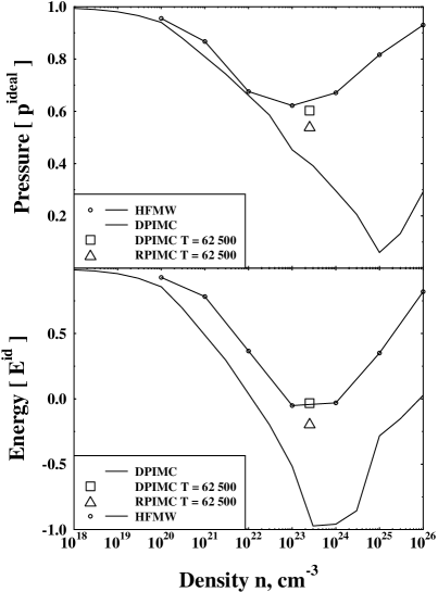
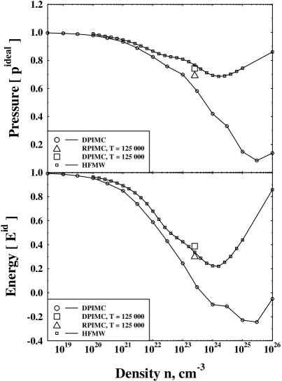
In this section we present results for the thermodynamic functions of dense hydrogen versus density at constant temperature. The PIMC simulations have been performed as explained in Filinov, V. S., et al. [2000], and Filinov V. S., et al. [2001]. Figures 1-3 show the simulation results together with the Padé results for three hydrogen isotherms $T=50,000$; $100,000$; and $125,000K$. In all figures the agreement between numerical and analytical data is good for temperatures and densities, where the coupling parameter $\Gamma$ is smaller than or equal to unity. Reference points related to RPIMC and DPIMC calculations in Fig. 1 correspond to data available for the temperature $T=62,500K$.

Figure 3: Energy and pressure isotherms for $125,000K$ (lower curves, solid line with larger or without circles). Solid line with smaller circles – Hartree Fock (HF) and Montroll–Ward (MW) approximation for $125000K$. Reference data: triangles – RPIMC (see Militzer et al. [2000]).

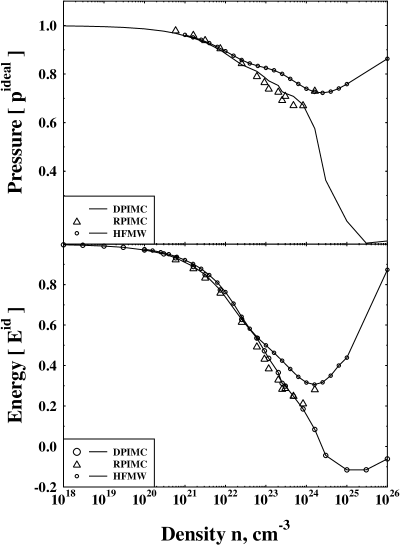
At low densities, pressure and energy are close to those of an ideal plasma. Increasing the density above $10^{19}cm^{-3}$, Coulomb interaction becomes important leading to a decrease of pressure and energy. Differences between analytical and numerical calculations in Fig. 1 are observed for densities above $10^{22}$ $cm^{-3}$ where the coupling parameter $\Gamma$ exceeds unity. At temperatures of $100,000$ and $125,000K$, differences are observed for $n$ above $5\times 10^{22}cm^{-3}$. The degeneracy parameter $n_{e}\lambda^{3}$ reaches here values of $0.4$. At higher densities (around $10^{24}cm^{-3}$) the degeneracy $n_{e}\lambda^{3}$ becomes larger than unity, and the interaction parts of pressure and energy decrease as compared to the respective ideal contributions, which leads to an increase of pressure and energy. At lower temperatures, this tendency is accompanied by the vanishing of bound states, i.e., a transition from a partially ionized plasma to a metal–like state. This tendency is correctly reproduced by all methods, however the density values of this increase vary. In Fig. 3 we compare our results with data from RPIMC simulations (see Militzer et al [2000]). Obviously, the agreement is very good up to densities below $10^{24}cm^{-3}$.

5 Discussion

This work is devoted to a Quantum Monte Carlo study of a correlated proton-electron system with degenerate electrons. We compared our direct PIMC simulations with independent restricted PIMC results of Militzer and Ceperley and analytical formulae for isotherms corresponding to $T=50,000$; $100,000$; and $125,000K$. The values of $\Gamma$ and $n_{e}\Lambda_{e}^{3}$ are varying in a wide range of values. This region is of particular interest as here pressure and temperature ionization occur and, therefore, an accurate and consistent treatment of scattering and bound states is crucial. We found that the results agree sufficiently well for coupling parameters smaller or equal to unity. This is remarkable because analytical formulae, the DPIMC and RPIMC simulations are completely independent and use essentially different approximations. We, therefore, expect that these results for hydrogen are reliable which is the main result of the present paper. We hope that our simulation results allow us to derive and test improved analytical approximations in the future.

6 Acknowledgements

We acknowledge support by the Deutsche Forschungsgemeinschaft (Sonderfor-
schungsbereich 198: M.B., D.K., and W.D.K; Mercator-Programm: V.S.F.). Our thanks are due to W. Ebeling and M. Schlanges for stimulating discussions.

References

• [1986] Kraeft, W.D., Kremp, D., Ebeling, W., Röpke, G.: Quantum Statistics of Charged Particle Systems, Akademie-Verlag Berlin and Plenum New York 1986
• [1997] Da Silva, I.B. et al.,: Phys. Rev. Lett. 78 (1997) 783
• [1995] Schlanges, M., Bonitz, M., Tschtschjan, A.: Contrib. Plasma Phys. 35 (1995)109
• [2000] Bonitz, M., (Ed.): Progress in Nonequlibrium Green’s functions, World Scientific, Singapore 2000
• [1977] Zamalin, V.M., Norman, G. E., Filinov, V. S.: The Monte Carlo Method in Statistical Thermodynamics, Nauka, Moscow 1977 (in Russian).
• [2000] Filinov, A. V., Lozovik, Yu. E., Bonitz, M.: phys. stat. sol. (b) 221 (2000) 231; Filinov, A. V., Bonitz, M., Lozovik, Yu. E.: Phys. Rev. Lett. (2001), arXiv:cond-mat/0012265
• [2000] Militzer, B., Pollock, E.: Phys. Rev. E 61 (2000) 3470
• [2000] Militzer, B., Ceperley, D.: Phys. Rev. Lett. 85 (2000) 1890
• [2000] Militzer, B., PhD-Thesis, University of Illinois (2000)
• [2000] Filinov, V. S., Bonitz, M., Fortov, V. E.: JETP Letters, 72 (2000) 245; Filinov, V. S., Fortov, V. E., Bonitz, M., Kremp, D.: Phys. Lett. A 274 (2000) 228
• [2001] Filinov, V. S., Bonitz, M., Ebeling, W., Fortov, V. E.: Plasma Phys. Contr. Fusion (2001)
• [1965] Feynman, R. P., Hibbs, A. R.: Quantum mechanics and path integrals, 1965, McGraw-Hill, New York.
• [1964] Kelbg, G.: Ann. Physik, 12 (1963) 219; 13 (1964) 354; 14 (1964) 394
• [1981] Ebeling, W., Richert, W., Kraeft, W. D., Stolzmann, W.: phys.stat.sol.(b) 104 (1981) 193
• [1987] Haronska, P., Kremp, D., Schlanges, M: Wiss. Z. Univ. Rostock, MN Reihe 36 (1987) 98
• [1985] Ebeling, W., Richert, W.: Phys. Lett. A 108 (1985) 80; phys. stat sol. (b) 128 (1985) 67