A one-dimensional toy model of globular clusters

Abstract

We introduce a one-dimensional toy model of globular clusters. The model is a version of the well-known gravitational sheets system, where we take additionally into account mass and energy loss by evaporation of stars at the boundaries. Numerical integration by the “exact” event-driven dynamics is performed, for initial uniform density and Gaussian random velocities. Two distinct quasi-stationary asymptotic regimes are attained, depending on the initial energy of the system. We guess the forms of the density and velocity profiles which fit numerical data extremely well and allow to perform an independent calculation of the self-consistent gravitational potential. Some power-laws for the asymptotic number of stars and for the collision times are suggested.

1	Department of Numerical Analysis and Computer Science, KTH,
	S-100 44 Stockholm, Sweden
2	Dipartimento di Fisica, Universitá di Roma “La Sapienza”,
	Piazzale Aldo Moro, 2 - I-00185 Roma, Italy
3	Dipartimento di Energetica “Sergio Stecco”, Universitá
	di Firenze, INFM and INFN, Via S. Marta, 3 - I-50139 Firenze, Italy

PACS numbers: 05.45.-a; 05.45.Pq; 98.10.+z; 98.20.Jp.

1 Introduction

Globular clusters are gravitationally bound concentrations of large numbers of stars, spherically distributed in space. They orbit around a galaxy spending most of the time in the galactic halo [1]. The most important elements governing globular clusters structure are two-body relaxation and truncation due to tidal forces. Different dynamical models considering these specific phenomena, have been investigated both analytically [1, 2, 3, 4] and numerically [5, 6, 7]. For an extended discussion, see [8] and Refs. therein.

Dynamical evolution causes stars to escape as an effect of the gravitational interaction with the nearby galaxies. This evaporation process drives the cluster towards a configuration with a high density core and the velocity dispersion of stars in the bulk can increase without limit. This phenomenon is known as gravothermal catastrophe and its study goes back to Antonov [9] and to Lynden-Bell and Wood [10].

Referring to the pioneering work of Chandrasekhar [1], it is possible to calculate the perturbations induced by stellar encounters on star motion. This is done by means of a diffusion model, which allows to derive a quantitative description of changes of star velocities in terms of single encounters. Considering weak encounters, i.e. solving the diffusion model in the Fokker-Planck approximation, King [4] found the following expression for the velocity profile

$$\left\{\begin{array}[]{ll}f_{0}(v)=A\left(\exp\left(\frac{-v^{2}}{2\sigma^{2}}\right)-\exp\left(\frac{-v_{c}^{2}}{2\sigma^{2}}\right)\right)&\mbox{for $v\leq v_{c}$}\\ \\ f_{0}=0&\mbox{for $v>v_{c}$,}\end{array}\right\}$$ (1)

where $v_{c}$ is a cutoff velocity of the stars, $\sigma$ is the one-dimensional velocity dispersion and $A$ a normalization constant. King’s models have been shown to be in agreement with the observed brightness surface profiles of globular clusters [4]. Further developments of King’s model [8] consider the same functional form (truncated Gaussian) applied to the gravitational energy, and hence propose a general form for the distribution function $f({\bf x},{\bf v})$. We will not consider here these extensions.

In this paper we discuss a simplified one-dimensional $N$-body model which reproduces King’s distribution. We let the particles, all of equal mass $m$, interact through the one-dimensional gravitational potential $V=2\pi Gm^{2}|x|$, where $G$ is the gravitational constant. Bearing in mind the comparison with globular clusters, we imitate the effect of galactic tidal forces by introducing a finite cut-off in positions. Thus, the evaporation of stars from the system is the only “dissipative” effect we consider. This is enough to drive the system towards an asymptotic non stationary regime, which we analyze in detail, and which reveals striking similarity with King’s model.

The main difference between the simplified one-dimensional model considered here and a more realistic three-dimensional one, is the lack of any singularity of the potential at the origin. The presence of a finite lower bound for the $1D$ potential makes less energy available to support the evaporation process as the system cools down. In the $3D$ case an infinite amount of energy can indeed be extracted from the singular pair-wise gravitational interaction, which is the main origin of the gravothermal catastrophe. This is the reason why the model we discuss cannot reproduce the core collapse corresponding to the gravothermal catastrophe.

In the next Section we present the model and the results concerning velocity distribution and density profiles. Section 3 is devoted to the discussion of power-laws for the number of particles in the cluster. Finally, in Section 4 we draw some conclusions.

2 One-dimensional model

Let us consider a one-dimensional classical Newtonian self-gravitating system of $N$ particles with equal mass $m$, with Hamiltonian [11]

$$H=\frac{1}{2}m\sum_{i}^{N}v^{2}_{i}+2\pi Gm^{2}\sum_{j<i}|x_{i}-x_{j}|~{},$$ (2)

where $x_{i}$ is the position and $v_{i}$ the velocity of $i$-th star. $G$ is the universal gravitational constant. We choose in the following $m=1$ and $2\pi G=1$. This system has been recently the subject of intensive investigations [12]. Particle accelerations are constant inbetween two collisions and are proportional to the net difference of particles respectively on the right and on the left. When a collision occurs particles cross each other, or, equivalently, collisions are elastic. This particle approach is known to corresponds in the continuum limit ($N\to\infty$) to the Vlasov-Poisson equations for the distribution function $f(x,v)$

$$\frac{\partial f}{\partial t}+v\frac{\partial f}{\partial x}-\frac{\partial V}{\partial x}\frac{\partial f}{\partial v}=0$$

$$\frac{\partial^{2}V}{\partial x^{2}}=4\pi Gm\int f(x,v)dv~{},$$ (3)

where $V(x)$ is the self-consistent gravitational potential.

We add the following features to the model

• Particles are confined in a box of size $L$, i.e. $x_{i}\in[-L/2,L/2]$

• The effect of tidal forces induced by the parent galaxy is imitated by requiring that each time a particle reaches the boundary of the box with a finite velocity, it drops out of the system, which therefore experiences a mass and energy loss (“evaporation”). This last feature implies that system (3) is solved with absorbing boundary conditions.

The numerical implementation is based on an “event-driven” scheme, first introduced in plasma physics [13], which is adapted to the present case as follows. The algorithm looks for the particles which collide the first and for the time when the event occurs, $t_{coll}$. Then it computes the first “evaporation time”, $t_{evap}$, and makes the system evolve until the minimum, $t_{min}$, between the collision and the evaporation time is reached. Once the system experiences evaporation, the total mass is reduced and the escaping particle stops interacting with the residual bulk. By rescaling the position and the velocity of each particle, i.e. introducing a local dissipation, we maintain the position of the center of mass fixed and its velocity to zero. This means we simply translate velocity and position of the remaining particles to keep the system centered in position and momentum space. A particle can escape from the system as a result of this rescaling: this possibility is taken into account even if it is has a low probability.

Evaporation is a singular event, which, in fact, marks the transition between two self-gravitating system having a different number of particles and energy. We remark that the integration scheme is “exact”. Time $t$ elapsed from the initial configuration is obtained by summing all values of $t_{min}$ up to the last event.

In all numerical experiments, $N(0)$ particles are initially uniformly distributed in the box and the initial velocities are Gaussian i.i.d random variables, with the temperature $T_{0}$ given by twice the average kinetic energy.

In Fig. 1 we show the time evolution of the number of particles $N(t)$ which remain inside the box up to time $t$. After an abrupt decrease of $N(t)$, which strongly depends on the initial condition, the system reaches a state where rare evaporations are present, making $N(t)$ decrease much slowlier. Our numerical experiments show that such a quasi-stationary state lives indefinitely, although we cannot exclude that, finally, $N(t)$ relaxes to an asymptotic value $N_{as}$. As the best approximation for this value, we take the one the system reaches in the longest computer runs.

Given $L$, for large enough $T_{0}$ the system approaches a state characterized by a single cluster, which adapts itself to the size of the box. In Fig. 2 we show the phase-space portrait for a system in its late stage evolution, when the most energetic particles have dropped out from the box and the system has relaxed to an asymptotic plateau, as the ones reported in Fig. 1. The particles are almost uniformly distributed within a bounded region of the phase plane. Both this fact and the shape of the contour suggest a possible connection with the so called water-bag (WB) distribution [11, 14]. This is a stationary solution of the Vlasov-Poisson system (3), $f^{WB}(x,v)$, which is constant in a simply connected domain $\Omega$ of the phase-plane and strictly zero outside.

Adopting the notation of Ref. [11], we call respectively $x_{s}$ and $v_{s}$ the maximum position and velocity of the WB. The potential $V(x)$ for such a distribution is then implicitly specified by the following integral equation

$$x=\frac{\epsilon^{\frac{3}{4}}}{N_{as}}\int^{V(x)}_{0}\left[\epsilon^{\frac{3}{2}}-(\epsilon-\zeta)^{\frac{3}{2}}\right]^{-\frac{1}{2}}d\zeta~{}.$$ (4)

The maximal energy of the water-bag, $\epsilon$, is such that, if we express $f(x,v)$ in terms of the energy $u=v^{2}/2+V(x)$, $f(x,v)=F(u)=0$ if $u>\epsilon$. The energy $\epsilon$ is related to $x_{s}$ and $v_{s}$ by $\epsilon=v_{s}^{2}/2$, $V(x_{s})=\epsilon$ and the zero energy level is fixed by requiring that $V(0)=0$. The density profile, $\rho^{WB}(x)$, is expressed as function of the potential

$$\rho^{WB}(x)=\frac{3N_{as}^{2}}{8\epsilon^{3/2}}(\epsilon-V)^{1/2}~{}.$$ (5)

Since the distribution function $f(x,v)$ is constant over $\Omega$, it follows immediately

$$\rho^{WB}(x)=\int^{v^{+}(x)}_{-v^{+}(x)}f(x,v)dv=2cv^{+}(x)$$ (6)

where $v^{+}(x)$ represents the profile of the upper branch of the WB contour, which we assumed to be symmetric, and $c=3N_{as}^{2}/(16\sqrt{2}\epsilon^{3/2})$. Using Eq. (5), this implies

$$v^{+}(x)=\sqrt{2(\epsilon-V)}~{}.$$ (7)

To compute the velocity contour $v^{+}(x)$, we need to know $V(x)$, which we do by solving Eq. (4) by an adaptive recursive Newton-Cotes 8 panel rule with tolerance $10^{-7}$. This velocity contour is drawn in Fig. 2 and, as predicted, encloses all phase points. In deriving $V(x)$ we have taken the value $v_{s}$ from the cluster phase plot; this is the only phenomenological input in this calculation and the agreement with the data has to be considered quite satisfactory.

Moreover, we can compare the theoretically derived potential $V(x)$ with the one computed directly from the asymptotic positions

$$V(x_{i})=\sum_{j}|x_{i}-x_{j}|~{}.$$ (8)

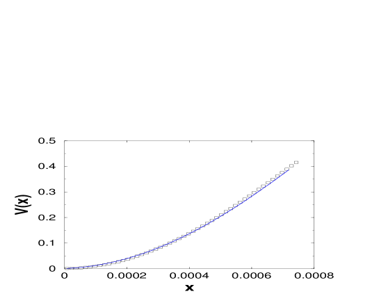
Figure 3: Gravitational potential calculated numerically using Eq. (8) (squares) and analytically by solving the integral equation (4) with $v_{s}=0.88$ (full line). Only the region of positive $x$ is drawn, in arbitrary units.

We need, of course, to perform a vertical shift to fix the zero in the origin. The result of formula (8) is reported in Fig. 3 together with the theoretically derived potential. The agreement is really good. We are thus led to conclude that our asymptotic state is well described by a water-bag. However, this latter is a stationary solution of the self-gravitating 1D system, while in our simulations we continue to observe some particle evaporations even at very long times. This is why we have called our asymptotic state quasi-stationary and its description in terms of a water-bag distribution can only be approximate.

An alternative treatment of the asymptotic state is based on King’s formula (1). In this case one does not try to reproduce the full distribution function, but just its projections along the $x$ and $v$ axis: $\rho(x)=\int fdv$ and $f_{0}(v)=\int fdx$. Following the standard derivation of the equilibrium isothermal distribution [15], we are led to introduce an analytical ansätz for the density profile

$$\left\{\begin{array}[]{ll}\rho(x)=A({cosh^{-2}(Bx)}-{cosh^{-2}(B\frac{L}{2})})&\mbox{for $|x|<\frac{L}{2}$}\\ \\ \\ \rho(x)=0&\mbox{for $|x|>\frac{L}{2}$~{},}\end{array}\right\}$$ (9)

where the normalization $A$ is fixed by $\int_{-L/2}^{L/2}\rho(x)dx=N_{as}$. For the velocities we take King’s distribution, specified in Eq. (1). Assuming $\rho(x)$ as in Eq. (9) we can derive a close analytical expression for the potential. For a one-dimensional system, the following relation holds in the continuum limit

$$V(x)=\int^{\frac{L}{2}}_{-\frac{L}{2}}|y-x|\rho(y)dy~{}.$$ (10)

Inserting Eq. (9) into Eq. (10) and performing the integral, we get

$$V(x)=\\ V_{0}\left[\frac{L}{B}\tanh(B\frac{L}{2})-(x^{2}+\frac{L^{2}}{4})\cosh^{-2}(B\frac{L}{2})+\\ \\ \frac{2}{B^{2}}\ln(\frac{\cosh(Bx)}{\cosh(B\frac{L}{2})})\right]~{},$$ (11)

with

$$V_{0}=\frac{N}{\frac{2}{B}\tanh(B\frac{L}{2})-L\cosh^{-2}(B\frac{L}{2})}~{}.$$ (12)

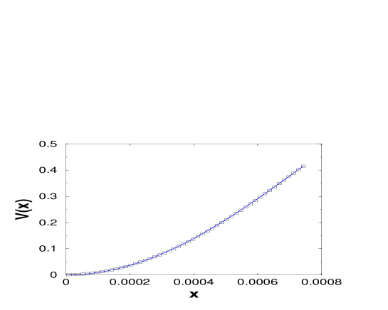
Figure 4: Gravitational potential calculated numerically using Eq. (8) (squares) and by a numerical fit which uses Eq. (11) (full line), where $B=731.2$ is the only free parameter.

$V(x)$ is quadratic for small $x$. To verify the reliability of our guess we re-analyze the data previously discussed in connection with the water-bag distribution. In Fig. 4 we plot the potential calculated numerically from Eq. (8) together with a one-parameter fit, using Eq. (11). Again the agreement with the data is very good and even apparently superior to the one obtained using the WB picture. This is simply due to the fact that here we perform a one parameter fit, while, in the previous discussion, $v_{s}$ was arbitrarily deduced from the phase space analysis. As a cross-check, we introduce in Eq. (9) the coefficient $B$ determined from the fit of the potential. The resulting density profile is plotted in Fig. 5 and it agrees with the normalized histogram of particles position. Finally, an histogram of the velocity is represented in Fig. 6. The reverse-cup shape due to the cut-off of the tails is evident. The solid line in Fig. 6 is a numerical fit which uses the expression of Eq. (1) with $v_{c}$ and $\sigma$ as free parameters.

As a side remark we observe that, coherently with the observed form of the potential, each particle oscillates almost harmonically inside the box. This can be seen by looking at the asymptotic orbit of a single particle (Fig. 7). The slight diffusion of the orbit is the signature of the interaction with the other particles, which induces a weak chaoticity.

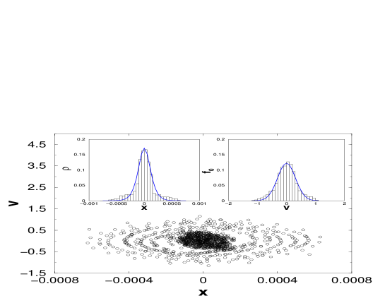
Figure 8: Phase-space plot for a system of $N(0)=1500$ particles after $30\times 10^{6}$ collisions. Here $T_{0}=0.02$, $L=0.0015$ and $N_{as}=1167$. Left insert: normalized histogram of positions. The solid line is a fit which uses Eq. (9) where $B=6845.7$. Right insert: normalized histogram of velocities. The solid line is the fit obtained using Eq. (1) with $\sigma=0.3$, $v_{c}=1.9$. All quantities are expressed in arbitrary units.

A further aspect that we have tested is the dependence of the dynamics on the initial temperature, $T_{0}$. Indeed, for small values of $T_{0}$, the system shows a pronounced collapse, which leads to a massive central core, as it is clearly displayed in the main plot of Fig. 8. This phase-space distribution significantly differs from the one in Fig. 2 and cannot be represented by a water-bag. The histograms of positions and velocities are computed and plotted in the right and left inserts, respectively. Both the density and the velocity profiles are very well reproduced by a numerical fit based on our ansätz (9) and on King’s distribution (1).

In conclusion, the ansätz we have introduced shows a good agreement with numerical data for all values of $T_{0}$ we have simulated, while the water-bag distribution fails to reproduce the velocity and density profiles at very low initial temperature. However, in the high temperature range, the water-bag treatment is superior, because it leads to an accurate description of the full distribution $f(x,v)$.

3 Scaling laws

In this Section we discuss some numerically found scaling laws which do not have presently a theoretical justification but which are an important signature of the presence of a finite box.

We follow the system until it reaches the asymptotic state. Being $N_{coll}$ the number of collisions, we define the “average collision time”, $\tau=\frac{t}{N_{coll}}$.

In the main plot of Fig 9 we represent $N_{as}$ as a function of $\tau$. Each point refers to a different value of the initial temperature $T_{0}$, varying form $0.2$ to $7$, while $N_{coll}$ is maintained constant for each realization. The initial temperature controls the rate of evaporation at a very early stage of the evolution. Larger values of $T_{0}$, produce higher mass loss, inducing the system to relax to a quasi-stationary state characterized by less residual particles $N_{as}$ (see Fig. 1). This process has consequences at the dynamical level, determining a larger mean free path and consequently a larger value of $\tau$. The curve in Fig 9 is consistent with this qualitative picture, showing a power-law decay with exponents $a=-0.4$ which is valid over more than two decades. In the insert of Fig. 9, we plot $\tau$ vs. $T_{0}$.

We have also checked the dependence on $N$ of the collision time $t_{coll}$, defined as an average of all the collision times corresponding to each fixed value of $N$, i.e. inbetween two successive evaporations. In Fig. 10 we plot the results of different numerical experiments where we vary the initial temperature $T_{0}$. The dependence of $t_{coll}$ on $N$ is again a power-law with exponent $b=-2.5$. Note that $b\sim 1/a$, hence Fig. 9 can be thought as a macroscopic averaged image of the microscopic properties shown in Fig. 10.

4 Conclusions

We have introduced a one-dimensional toy model of globular clusters with an emphasis on the evaporation process. With this in mind, we have discussed the effect of introducing a finite size box in a classical one dimensional self-gravitating medium. The dynamics of the system has been investigated for a special class of initial conditions. We pointed out the appearance of two distinct, non stationary, asymptotic regimes which occur depending on the temperature of the initial realization. For small values of $T_{0}$, similarities with the isothermal solution are found while for larger temperatures the density and velocity profiles are well reproduced also assuming a water-bag distribution.

We propose a form of the density profile, with a cut-off in the tails, which fits well numerical data in all the explored regimes, allowing to derive a close analytical expression of the gravitational potential. Moreover, a King-like velocity profile is shown to be in good agreement with numerical data. The asymptotic truncated profiles are thus a direct consequence of the evaporation from the finite box.

Finally we have also given numerical evidence of some scaling laws, which remain to be theoretically explained, but which are strongly related to the escaping process.

In the future, we plan to extend this study to the system of concentric spherical mass shells [2] by introducing an external absorbing boundary in the configuration space as done here.

Acknowledgements We thank an anonymous referee for his helpful comments, which led to a substantial improvement of this paper. We acknowledge useful discussions with E. Aurell, M.C. Firpo, M. Henon and A. Noullez. This work is part of the MURST-COFIN00 grant on Chaos and localization in quantum and classical mechanics. D.F. warmly acknowledges the research group Dynamics of Complex Systems in Florence for the kind hospitality.

Figure 1: Plots of $N$ vs. $time$ for increasing initial temperatures, with $N(0)=400$. Temperature and time are expressed in arbitrary units.

Figure 2: Phase-space plot for a system of $N(0)=1500$ particles after $30\times 10^{6}$ collisions. Here $T_{0}=0.4$, $L=0.0015$ and $N_{as}=886$. The quantities $x$ and $v$ are expressed in arbitrary units. The full line which contains all the points is the theoretical prediction (7)

Figure 5: Normalized histogram of positions as derived from the phase-space plot in Fig. 2. The solid line is Eq. (9), with $B=731.2$ as previously. Position $x$ is expressed in arbitrary units.

Figure 6: Normalized histogram of velocities as derived from the phase-space plot in Fig. 2. The solid line is the fit obtained using Eq. (1) with $\sigma=0.87,v_{c}=0.98$. Velocity $v$ is expressed in arbitrary units.

Figure 7: Asymptotic orbit of a single particle for $N(0)=600$, $L=0.0035$. Positions and velocities are expressed in arbitrary units.

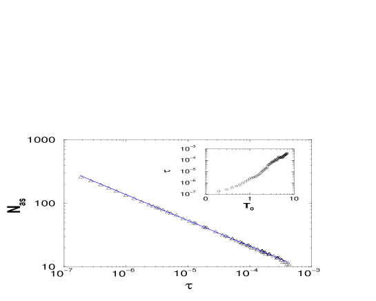
Figure 9: $N_{as}$ vs. $\tau$ in log-log scale. Here $\tau$ is defined as the ratio $\frac{t}{N_{coll}}$. Each point refers to a different $T_{0}$ while $N_{coll}$ is fixed. The solid line represents a power-law fit with the slope $a=-0.4$. In the upper right corner insert $\tau$ vs. $T_{0}$ is represented in a log-log scale. The quantities $T_{0}$ and $\tau$ are expressed in arbitrary units.

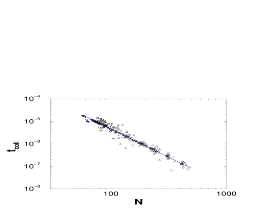
Figure 10: $t_{coll}$ vs. $N$ in log-log scale for $N(0)=600$ $L=0.0035$. Different symbols refer to different initial values of the temperature $T_{0}$. $t_{coll}$ is expressed in arbitrary units.

References

- [1] Chandrasekhar S., Astroph. J., 97, 263 (1943) and Astroph. J., 98, 54 (1943); Chandrasekhar S., An introduction to the study of stellar structure, University of Chicago Press, Chicago (1943).
- [2] Henon M., Ann. Astrophys., 27, 82 (1964); Bull. Astron., 3, 241 (1968).
- [3] Inagaki, S., Lynden-Bell, D., Mon. Not. R. Astr. Soc., 205, 913 (1983); Mon. Not. R. Astr. Soc., 244, 254 (1990);
- [4] King I., Astron. J., 67, 471 (1962); Astron. J., 70, 376 (1965); Astron. J., 71, 471 (1966).
- [5] Cohn H., Astroph. J., 242, 765 (1980).
- [6] Inagaki, S., Wiyanto, P., Publications of the Astronomical Society of Japan , 36, 391 (1984); Inagaki, S., Publications of the Astronomical Society of Japan, 38, 853 (1986); Inagaki, S., Saslaw, W. C., Astroph. J., 292, 339 (1985).
- [7] Miller B.N., Youngkins P., Phys. Rev. Lett., 81 4794 (1998).
- [8] Meylan G., Heggie D., Astron. Astrophys. Rev., 8, 1 (1997).
- [9] Antonov V.A., Vest Leningrad Univ., 7, 135 (1962).
- [10] Lynden-Bell D., Wood, R., Month. Not. Roy. Astr. Soc., 138, 495 (1968).
- [11] Hohl F. and Feix M.R., Astrophys. J., 147, 1164 (1967).
- [12] Reidl C.J., Miller B.N., Phys. Rev. A, 46, 837 (1992); Phys. Rev. E, 48, 4250 (1993); Tsuchiya T., Konishi T., Gouda N., Phys. Rev. E, 50, 2607 (1994);Tsuchiya T., Gouda N., Konishi T., Phys. Rev. E, 53, 2210 (1996); Milanovic Lj., Posch H.A., Thirring W., Phys. Rev. E, 57, 2763 (1998).
- [13] Eldridge O.C. and Feix M.,The Physics of Fluids, 5, 1076 (1962).
- [14] De Packh D.C., J. Electr. Contr., 13, 417 (1962).
- [15] Rybicki G.B., Astrophys. Space Sci., 14, 56 (1971)