Application of a relativistic accretion disc model to X-ray spectra of LMC X-1 and GRO J1655–40

Abstract

We present a general relativistic accretion disc model and its application to the soft-state X-ray spectra of black hole binaries. The model assumes a flat, optically thick disc around a rotating Kerr black hole. The disc locally radiates away the dissipated energy as a blackbody. Special and general relativistic effects influencing photons emitted by the disc are taken into account. The emerging spectrum, as seen by a distant observer, is parametrized by the black hole mass and spin, the accretion rate, the disc inclination angle and the inner disc radius.

We fit the ASCA soft state X-ray spectra of LMC X-1 and GRO J1655–40 by this model. We find that having additional limits on the black hole mass and inclination angle from optical/UV observations, we can constrain the black hole spin from X-ray data. In LMC X-1 the constrain is weak, we can only rule out the maximally rotating black hole. In GRO J1655–40 we can limit the spin much better, and we find $0.68\leq a\leq 0.88$. Accretion discs in both sources are radiation pressure dominated. We don’t find Compton reflection features in the spectra of any of these objects.

1 Introduction

Black hole binaries (BHB) are generally observed in one of the two spectral states, as determined by their X-ray/$\gamma$-ray energy spectra. In the hard state most of energy is radiated above $\sim$ 10 keV. The spectrum is dominated by a power law with the photon spectral index $\Gamma<2.0$ and a high-energy cutoff above 100 keV (Grove et al. 1998). A common interpretation of this emission is in terms of Comptonization of soft seed photons by thermal, hot, optically-thin electron plasma. Cyg X-1 (Gierliński et al. 1997) and GX339–4 (Zdziarski et al. 1998) are typical examples of the hard state BHB. In the soft state most of the energy is radiated in the soft X-rays, below $\sim$ 10 keV. This energy range is dominated by a blackbody-like component with characteristic temperature $\sim$ 1 keV. This component is usually attributed to the thermal emission of a cold, optically-thick accretion disc, extending down to the marginally stable orbit (Shakura & Sunyaev 1973). The disc spectrum is often accompanied by a high-energy tail, which can be described as a power law with a typical photon spectral index $\Gamma\sim 2.0$–$2.5$, extending into $\gamma$-rays without apparent break or cutoff (Grove et al. 1998). LMC X-1 (Schlegel et al. 1994), LMC X-3 (Ebisawa et al. 1993), GS 1124–68 just after the outburst (Ebisawa et al. 1994) or Cyg X-1 between May and August 1996 (Gierliński et al. 1999) are the examples of the soft state BHB.

At first approximation the soft component in the soft state can be described by a multicolour disc model (hereafter MCD; Mitsuda et al. 1984), which spectrum is a sum of blackbodies with radial temperature distribution $T(r)\propto r^{-3/4}$. This model has been commonly used for spectral fitting by many authors. Though MCD model approximates the disc spectral shape well, it ignores the inner torque-free boundary condition and parameters derived through it are incorrect. An improvement of the MCD model is a multicolour disc model in the pseudo-Newtonian potential (Gierliński et al. 1999), taking properly into account the boundary condition.

In vicinity of the black hole relativistic effects become important. The effects of relativity on the emerging disc spectrum have been studied by Cunningham (1975), Laor, Netzer & Piran (1990), Asaoka (1989), Hanawa (1989), Fu & Taam (1990), Yamada et al. (1994) and others. Hanawa (1989) calculated disc spectra around a non-rotating black hole, creating a fast-computing model that have been used for spectral fitting several times (e.g. Ebisawa, Mitsuda & Hanawa 1991; Makishima et al. 2000). However, this model is limited to Schwarzschild metric only and effects of light bending have been neglected. More advanced model was developed by Laor et al. (1990), who studied accretion discs around rotating black hole, taking into account both relativistic effects affecting radiation and vertical structure of the disc. Laor (1990) applied this model to the AGN spectra.

In this paper we show an application of the general relativistic (hereafter GR) disc model to the soft state X-ray spectra of BHB. We focus on estimating the black hole spin. The model thoroughly treats relativistic effects in the deep gravitational potential of the black hole. In Section 2 we give description of the model and show examples of the model spectra. Then, we fit the X-ray spectral data of LMC X-1 (Section 3.1) and GRO J1655–40 (Section 3.2) with the GR model. In Section 4 we discuss the obtained results.

2 Model description

We consider an accretion disc around a black hole (e.g. Page & Thorne 1974). The model is based upon certain assumptions. We assume that the disc rotates in the equatorial plane around the Kerr black hole; that it is in a steady state; that it is axially symmetric; that it is flat and geometrically thin; that it is optically thick; that it locally radiates away the dissipated gravitational energy as a blackbody; that there is no emission below the marginally stable orbit.

A black hole is characterized by its mass, $M$, and angular momentum, $J$. We use dimensionless spin $a\equiv Jc/GM^{2}$, where $0\leq a\leq 1$ and $a=0$ corresponds to the non-rotating (Schwarzschild) black hole. In accreting systems the radiation emitted by the disc produces a counteracting torque and the black hole cannot be spun-up beyond $a=0.998$ (Thorne 1974). Therefore we do not exceed this value in our model and refer to it as to the maximally rotating black hole. The efficiency of accretion, $\eta$, varies from $\eta\approx 0.057$ for the non-rotating black hole to $\eta\approx 0.32$ for $a=0.998$.

The spectrum of the disc, $F_{\nu}$, seen at infinity is computed by means of a photon transfer function, $\cal T$, which describes travel of photons from the point of origin to the distant observer. The photon of frequency $\nu_{e}$ is emitted at radius $r_{e}$, at cosine angle $\mu_{e}\equiv\cos\theta_{e}$ and then perceived at frequency $\nu_{o}$ by the observer at cosine angle $\mu_{o}\equiv\cos i$. The observed flux is

$$F_{\nu_{o}}(\mu_{o})=\left(R_{g}\over D\right)^{2}\nu_{o}\!\int\!\!{\rm d}g_{\rm eff}\!\!\int\!\!{\rm d}r_{e}\!\!\int\!\!{\rm d}\mu_{e}\,$$

$$~{}~{}~{}~{}\times r\,{\cal T}(a,r_{e},\mu_{e},g_{\rm eff},\mu_{o})\,N(r_{e},\mu_{e},{\nu_{o}\over g_{\rm eff}}).$$ (1)

Subscript ‘$e$’ denotes quantities measured in the local frame co-moving with the disc and subscript ‘$o$’ denotes quantities measured by the observer at infinity. $N(r_{e},\mu_{e},{\nu_{o}\over g_{\rm eff}})\equiv N_{\nu_{e}}(r_{e},\mu_{e})$ is the specific photon number intensity of the disc emission, $g_{\rm eff}\equiv\nu_{o}/\nu_{e}$ is the effective redshift of the photon, $D$ is the distance to the source and $R_{g}\equiv GM/c^{2}$ is the gravitational radius. Numerical constants are included in the transfer function.

The transfer function treats the special and general relativistic effects affecting the spectrum. It takes into account the Doppler energy shift from the fast moving matter in the disc, the gravitational shift and the light bending near the massive object. It includes integration over the azimuthal angle $\phi_{e}$. Each element of the transfer function, ${\cal T}(a,r_{e},\mu_{e},g_{\rm eff},\mu_{o})$, was computed by summing all photon trajectories for all angles $\phi_{e}$, at given ($r_{e}$, $\mu_{e}$), for which required ($g_{\rm eff}$, $\mu_{o}$) were obtained. The details of the transfer function computation are given in Appendix A. A similar approach to computing the black hole disc spectra has been applied, e.g., by Laor et al. (1990) and Asaoka (1989). Note that our construction of $\cal T$ is slightly different than that of Cunningham (1975), as the latter one involves the relation of the specific intensities at the emitter and the observer, respectively, given by Liouville’s theorem, while our model is based on counting individual photons.

The local gravitational energy release per unit area of the disc, per unit time is (Page & Thorne 1974)

$$Q(x)={3\dot{M}_{\rm d}c^{6}\over 8\pi G^{2}M^{2}}\,{1\over x^{4}(x^{3}-3x+2a)}\left[x-x_{0}-{3\over 2}a\ln\left({x\over x_{0}}\right)\right.$$ (2)

$$-{3(x_{1}-a)^{2}\over x_{1}(x_{1}-x_{2})(x_{1}-x_{3})}\ln\left({x-x_{1}\over x_{0}-x_{1}}\right)$$

$$-{3(x_{2}-a)^{2}\over x_{2}(x_{2}-x_{1})(x_{2}-x_{3})}\ln\left({x-x_{2}\over x_{0}-x_{2}}\right)$$

$$\left.-{3(x_{3}-a)^{2}\over x_{3}(x_{3}-x_{1})(x_{3}-x_{2})}\ln\left({x-x_{3}\over x_{0}-x_{3}}\right)\right],$$

where $x=r_{e}^{1/2}$, $x_{0}=r_{\rm ms}^{1/2}$, $x_{1}=2\cos({1\over 3}\arccos a-\pi/3)$, $x_{2}=2\cos({1\over 3}\arccos a+\pi/3)$ and $x_{3}=-2\cos({1\over 3}\arccos a)$.

$$r_{\rm ms}=3+A_{2}-{\rm sign}\,a\,\left[(3-A_{1})(3+A_{1}+2A_{2})\right]^{1/2}$$ (3)

is the marginally stable orbit radius, where $A_{1}=1+(1-a^{2})^{1/3}[(1+a)^{1/3}+(1-a)^{1/3}]$ and $A_{2}=(3a^{2}+A_{1}^{2})^{1/2}$. Both $r_{e}$ and $r_{\rm ms}$ are expressed in units of $R_{g}$.

The photon number intensity, $N_{\nu_{e}}$, can be derived from the energy release rate, $Q$. However, the relation between these two quantities is not simply $Q(r_{e})=\int h\nu_{e}N_{\nu_{e}}(r_{e},\mu_{e}){\rm d}\nu_{e}{\rm d}\mu_{e}$, as assumed in previous similar calculations (e.g., Laor et al. 1990). The photon number intensity which is used in equation (1), is defined in terms of the distant observer coordinate frame. On the other hand, $Q$ is defined as the energy dissipated per unit proper time per unit proper area, as measured by the observer orbiting with the disc. The corresponding dissipation rate measured by the distant observer will be affected by kinematic and gravitational time dilation and length contraction. We emphasize that these effects are not included in the calculation of the single photon trajectory, and are treated separately when applying the transfer function formalism.

In Appendix B we derive transformation of the time and the disc surface area between the disc rest frame and the frame of the distant observer:

$${\rm d}t^{\prime}=\beta_{t}{\rm d}t,~{}~{}~{}~{}~{}~{}~{}~{}~{}~{}~{}{\rm d}r^{\prime}{\rm d}\phi^{\prime}=\beta_{S}{\rm d}r{\rm d}\phi,$$ (4)

where $(t,r,\phi)$ and $(t^{\prime},r^{\prime},\phi^{\prime})$ are the coordinates of the reference frame of the distant observer and the disc, respectively.

In order to find a locally emitted spectrum we would need to compute the vertical structure of the disc. However, this problem did not find a satisfactory general solution yet. Instead, we simply assume that each point of the disc radiates like a blackbody and introduce two corrections. First, we note that the Thomson scattering dominates over absorption in the inner part of the disc and the local spectrum is affected by Comptonization. At a given radius, $r_{e}$, we approximate the spectrum by a diluted blackbody,

$$B_{\nu_{e}}^{\rm db}={1\over f_{\rm col}^{4}}B_{\nu_{e}}(f_{\rm col}T_{\rm eff}),$$ (5)

where $B_{\nu_{e}}$ is the Planck function, $f_{\rm col}=T_{\rm col}/T_{\rm eff}$ is the spectral hardening factor, $T_{\rm col}$ is locally observed colour temperature and $T_{\rm eff}$ is the effective temperature, related to the locally dissipated energy, $Q$, as $\sigma T_{\rm eff}^{4}=Q$. Following Shimura & Takahara (1995) we use $f_{\rm col}=1.7$.

The second correction concerns angular distribution of local emission. We assume a linear limb darkening in form:

$$I_{\nu_{e}}(\mu_{e})=I_{0}{1+\delta\mu_{e}\over 1+\delta}B_{\nu_{e}}^{\rm db},$$ (6)

where $\delta=2.06$ in classical electron scattering limit (e.g. Phillip & Mészáros 1986). $I_{\nu_{e}}$ is the specific intensity in the local frame, co-rotating with the disc. Factor $I_{0}$ is found from the requirement of energy conservation. Namely, the power emitted by a limb-darkened surface element d$A$, $2\pi\int_{0}^{1}I_{\nu_{e}}(\mu_{e})\mu_{e}$d$\mu_{e}$d$A$, should be equal to the power emitted by the same surface element without limb darkening, $\pi B_{\nu_{e}}^{\rm db}\,$d$A$. From this we find

$$I_{0}=3{1+\delta\over 3+2\delta},$$ (7)

and

$$I_{\nu_{e}}(\mu_{e})=3{1+\delta\mu_{e}\over 3+2\delta}B_{\nu_{e}}^{\rm db}.$$ (8)

Then, the specific photon number intensity of the disc, measured by the distant observer, is given by

$$N_{\nu_{e}}(\mu_{e})=\beta_{S}\beta_{t}{I_{\nu_{e}}(\mu_{e})\over h\nu_{e}}.$$ (9)

Figure 1: Spectra from the GR disc model for $a$ = 0, 0.25, 0.5, 0.75 and 0.998 (from the bottom to the top). The disc extends from the marginally stable orbit to $r_{\rm out}=10^{4}$. The spectra were computed for a 10M_⊙ black hole at 1 kpc, with accretion rate $\dot{M}_{\rm d}=10^{18}$ g s^-1, disc inclination angle $i=45^{\circ}$, $f_{\rm col}$ = 1.7 and $\delta$ = 2.06.

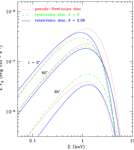
Figure 2: Comparison of the GR and PN disc models for different inclination angles. For both discs $r_{\rm in}=6$. The spectra were computed for a non-rotating 10M_⊙ black hole at 1 kpc, with accretion rate $\dot{M}_{\rm d}=10^{18}$ g s^-1, $f_{\rm col}$ = 1.7. The effect of the limb darkening in the relativistic disc is also shown.

There is, however, one effect that we have not taken into account. Due to gravitational focusing some of the emitted photons return to the disc, where they are reprocessed or scattered. Since the returning photons alter the locally emitted spectrum recurrently, taking them into account would require enormous computing time and would make spectral fitting practically impossible. In our model returning photons are lost, so the disc luminosity and temperature are underestimated for the spin close to maximum. This effect was studied by Cunningham (1976). He found that returning radiation is negligible for $a<0.9$. The difference between the actual locally generated flux and that in the absence of returning radiation is only a few per cent over most of the inner disc for the maximally rotating black hole. At lower spins, the effect is much less pronounced. In this paper we compute the GR disc spectra for $a$ = 0, 0.25, 0.5, 0.75 and 0.998. Though the $a=0.998$ model underestimates temperature and luminosity, the interpolation between the models would give accurate results for $a<0.9$, and slightly overestimated spin measurement otherwise.

Figure 1 shows the GR disc spectra for different values of the black hole spin. We clearly see how the accretion efficiency grows with increasing spin, when energy is dissipated deeper in the gravitational potential. On Figure 2 we compare spectra of the GR model (with $a=0$) and the pseudo-Newtonian (PN) model (Gierliński et al. 1999). The PN model approximates temperature distribution with good accuracy, but effects of Doppler and gravitational shifts, light bending and focusing are neglected and light propagates through flat space. With increasing inclination angle both energy of the peak and normalization of the relativistic disc spectrum (dashed curve) increase in compare to the PN disc spectrum (dotted curve), mostly due to Doppler shifts and increase of the apparent disc area. A similar effect was found by Fu & Taam (1990). On the same figure we also show the effect of the limb darkening (solid curve), enhancing the spectrum for lower and diminishing it for higher inclination angles. Next, we check how the parameters obtained with the PN model relate to these from the GR model. To do this, we created fake ASCA spectra using the GR model with the following parameters: $M=10$M_⊙, $a=0$, $\dot{M}_{\rm d}=10^{18}$ g s^-1, $D$ = 1 kpc, $r_{\rm in}=6$, $r_{\rm out}=10^{4}$, $f_{\rm col}=1.7$. The spectra were computed for $\delta=0$ and 2.06, for several inclination angles. Then, we fitted the PN disc model to the spectra finding the black hole mass and the accretion rate. The results are presented on Figure 3. If the limb darkening is taken into account in the generated data, the accretion rate obtained with the PN model is underestimated by factor $\sim$ 0.8, almost independently of the inclination angle. The mass estimation is exact at inclination $i\approx 45^{\circ}$, underestimated for higher and overestimated for lower inclination angles. We stress that these fits were performed for a non-rotating black hole only.

Zhang, Cui and Chen (1997a) investigated accretion onto a rotating black hole in an approximate way. They used the MCD model and applied GR corrections due to fractional change in the colour temperature and due to change in the integrated flux. As a result, they were able to constrain the black hole spin of a few BHB, including GRO J1655–40, which we will analyze in details in Section 3.2. For comparison, we have applied their method to the spectra created by our GR model. The result depends on the GR corrections applied. Since Zhang et al. (1997) tabulated these corrections for $a$ = 0 and 0.998 only, the discrepancies are largest for $a\sim 0.5$. In particular, for spectra generated by the GR model with $a$ = 0.998, 0.75 and 0.5, the approximate treatment yields $a$ = 0.95, 0.58 and 0.24, respectively. We however note, that with GR corrections calculated precisely for all spin and inclination angle values the approximate method can provide with reasonably accurate results.

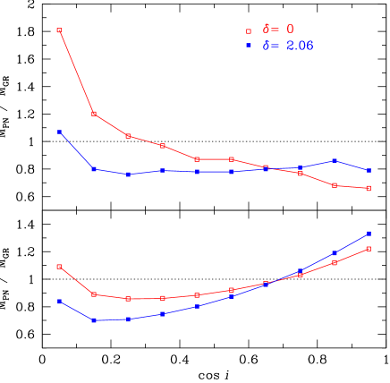
Figure 3: Fits of the pseudo-Newtonian disc model to the fake spectra generated from the GR model. The data were created for a non-rotating 10M_⊙ black hole with $\dot{M}_{\rm d}=10^{18}$ g s^-1 with (filled squares) and without (empty squares) limb darkening.

The relativistic disc model parameters are: the black hole mass, $M$, and its spin, $a$, the inner and outer disc radii, $r_{\rm in}$ and $r_{\rm out}$, respectively (in units of $R_{g}$), the accretion rate, $\dot{M}_{\rm d}$ and the inclination angle, $i$. Subscript ‘d’ denotes the accretion rate in the disc only, excluding all possible energy dissipation outside the disc. In our fits we always keep $r_{\rm out}=10^{4}$, so the model has at most 5 free parameters.

We underline that the overall model spectral shape does not change significantly, when these parameters vary. At first approximation, there are only two quantities fixing the spectrum: the energy of the peak in the spectrum (or the temperature) and the total flux (normalization). They translate into five model parameters, therefore only two out of them can be established uniquely. In most of our fits we fix $i$, $a$ and $r_{\rm in}$, leaving $M$ and $\dot{M}_{\rm d}$ as free parameters. As we show later, the inner disc radius as a free parameter can be also constrained to some extent.

However, the model, though unable to establish all parameters simultaneously, yields tight correlations between them. In particular, for a given spectrum and $r_{\rm in}=r_{\rm ms}$, as $a$ increases, $\dot{M}_{\rm d}$ decreases (to compensate the increased accretion efficiency) but $M$ increases (to keep the absolute inner disc radius $R_{\rm in}\propto r_{\rm in}M$ when $r_{\rm in}$ decreases). For a given spectrum and $a$ fixed, as $r_{\rm in}$ increases, $\dot{M}_{\rm d}$ increases but $M$ decreases. Having any additional restrictions for black hole mass and inclination angle we can hope to estimate the black hole spin.

3 Application to the data

For spectral fits, we use xspec v10 (Arnaud 1996). The confidence range of each model parameter is given for a 90 per cent confidence interval, i.e., $\Delta\chi^{2}=2.7$ (e.g. Press et al. 1992).

The X-ray spectra of both sources can be decomposed into two components: a soft, thermal emission peaking around a few keV and a high-energy tail. We interpret them in terms of an optically thick cold accretion disc and optically thin hot plasma. Therefore we fit the data by a model consisting of the GR disc and a high-energy tail, which we model either by a power law or by thermal Comptonization (see below). The model spectra are absorbed by the interstellar medium with a column density $N_{\rm H}$, for which we use the opacities of Bałucińska-Church & McCammon (1992) and the abundances of Anders & Grevesse (1989).

While constructing the disc model, we have tabulated the transfer function, $\cal T$, for five values of the black hole spin: $a$ = 0, 0.25, 0.5, 0.75 and 0.998. Since the radius of the marginally stable orbit, which is the lower limit of $r_{\rm in}$, is a function of $a$, we cannot interpolate between transfer functions tabulated for different values of $a$, when $r_{\rm in}$ is close to $r_{\rm ms}$. Therefore, we fit the data only for these five fixed values of $a$. In all the fits we keep the spectral hardening factor, $f_{\rm col}=1.7$ and the limb darkening factor $\delta$ = 2.06.

3.1 LMC X-1

3.1.1 Source properties

LMC X-1 is a luminous X-ray source in the Large Magellanic Cloud. It had been a long-standing controversy about the optical counterpart of the X-ray source, since the position of LMC X-1 established by Einstein was between two stars separated by only 6”. Cowley et al. (1995) improved the position of LMC X-1 from ROSAT-HRI observations and confirmed that the optical counterpart is a peculiar O7 III Star #32 with visual magnitude $V\sim 14.8$. Using optical spectroscopy Hutchings et al. (1987) showed that Star #32 is in a binary system with orbital period of 4.2288 days.

They found the mass function, $f_{M}=0.14\pm 0.05$M_⊙, and the lower limit for the mass of the compact object, $M>4$M_⊙, which makes LMC X-1 a good candidate for the stellar-mass black hole. The inclination angle of the binary is constrained by the lack of X-ray eclipses to be $i<63^{\circ}.5$. The mass ratio, $q\equiv M_{\ast}/M$ is greater than 2, which, together with the mass function yields

$$M\sin^{3}i>0.8{\rm M}_{\odot}.$$ (10)

The upper limit for the companion star is 25M_⊙, therefore $M<12.5$M_⊙ and $i>24^{\circ}$.

The distance to the Large Magellanic Cloud (LMC) is uncertain. It is usually published in terms of the distance modulus, $m-{\cal M}=5\log D_{\rm pc}-5$, where $m$ and ${\cal M}$ are apparent and absolute visual magnitudes and $D_{\rm pc}$ is the distance expressed in parsecs. Different determinations of the distance modulus result in conflicting results, from $18.065\pm 0.12$ (Stanek, Zaritsky & Harris 1998) to $18.7\pm 0.1$ (Feast & Catchpole 1997). This corresponds to the span in distance from 38.8 kpc to 57.5 kpc. Since the compact object mass determined from the disc observations depends linearly on $D$, this will significantly increase the uncertainty of mass determination.

The X-ray spectrum of LMC X-1 resembles the soft state spectrum of Cyg X-1 (Gierliński et al. 1999). At first approximation it can be represented by a blackbody with temperature $\sim 0.7$ keV and a high-energy power-law tail beyond the blackbody (e.g. Ebisawa, Mitsuda & Inoue 1989; Schlegel et al. 1994; Treves at al. 2000; Schmidtke, Ponder & Cowley 1999; Nowak et al. 2001). No transition to the hard state has been ever observed.

3.1.2 Spectral fits

LMC X-1 was observed by ASCA on April 2–3, 1995. We have extracted the SIS spectrum with the net exposure time of 23.6 ks. In our fits we use the 0.7–10 keV spectrum, except the channels between 1.8–2.2 keV, which are strongly affected by the instrumental gold feature. Since we are interested in the shape of the disc continuum, this small gap in energy channels will not affect our results.

Both the distance to LMC X-1, $D$, and the inclination angle of the system, $i$, are uncertain. In most of our fits we use $D=50$ kpc and $i=50^{\circ}$, but we also check our results within the acceptable range of $38.8$ kpc $<D<57.5$ kpc and $24^{\circ}<i<63^{\circ}.5$. We do not impose any constraints on the black hole mass, $M$, during the fits, but check its consistency with the limits obtained from the optical observations, $4.0$M${}_{\odot}\leq M\leq 12.5$M_⊙, a posteriori.

For the high-energy tail beyond the disc spectrum we chose a thermal Comptonization model (Zdziarski, Johnson & Magdziarz 1996). This model is fast and has few parameters, which makes it easy to use. We would like to stress that one important difference between the Comptonization model and a power law is the low-energy cutoff. The cutoff should be present in the Comptonized spectrum around the maximum disc temperature if the seed photons come from the disc. The soft power law, extending down towards lower energies without cutoff, may significantly affect measurements of the disc parameters.

Figure 4: The ASCA/SIS observation of LMC X-1 and a model with a non-rotating black hole (upper panel; see Table 1). The model (solid curve) is decomposed into the GR disc (dotted curve) and thermal Comptonization (dashed curve). The lower panel shows the data–model residuals divided by errors.

The Comptonization model has the following parameters: the electron temperature, $kT_{e}$, the asymptotic power-law photon spectral index, $\Gamma$, and the seed photons temperature, $kT_{\rm s}$. We have found that the electron temperature has a negligible effect on the fit results, so we keep it at 50 keV during our fits. We note, that due to lack of the data above 10 keV we cannot constrain plasma parameters, and we treat the Comptonization model only as a phenomenological component supplementary to the disc model. It is not our intention to study the hot plasma properties in this paper.

Table 1: Fit results of the GR disc plus thermal Comptonization model to LMC X-1 ASCA/SIS data for five different values of the black hole spin. The inclination angle is $i=50^{\circ}$ and the distance to the source $D$ = 50 kpc. The disc extends from $r_{\rm in}=r_{\rm ms}$ to $r_{\rm out}=10^{4}$. The disc and Comptonization models are described in Sections 2 and 3.1.2, respectively. $\dot{M}_{\rm d}$ denotes accretion rate in the disc (excluding power dissipated in the hot phase).

$a$	0.00	0.25	0.50	0.75	0.998
$N_{\rm H}$ ($10^{21}$ cm-2)	$5.35_{-0.19}^{+0.15}$	$5.33_{-0.18}^{+0.16}$	$5.34_{-0.19}^{+0.15}$	$5.35_{-0.19}^{+0.16}$	$5.41_{-0.20}^{+0.16}$
$\Gamma$	$3.29_{-0.50}^{+0.37}$	$3.30_{-0.44}^{+0.38}$	$3.36_{-0.39}^{+0.35}$	$3.43_{-0.34}^{+0.31}$	$3.48_{-0.22}^{+0.28}$
$kT_{\rm s}$ (keV)	$0.53_{-0.07}^{+0.04}$	$0.52_{-0.06}^{+0.05}$	$0.52_{-0.05}^{+0.04}$	$0.51_{-0.04}^{+0.05}$	$0.51_{-0.04}^{+0.03}$
$M$ (M⊙)	$9.7_{-1.6}^{+1.5}$	$11.3_{-1.7}^{+2.1}$	$14.2_{-2.3}^{+2.7}$	$20.0_{-3.4}^{+3.8}$	$45_{-8}^{+9}$
$\dot{M}_{\rm d}$ ($10^{18}$ g s-1)	$3.7_{-0.8}^{+0.8}$	$3.1_{-0.7}^{+0.7}$	$2.5_{-0.5}^{+0.5}$	$1.9_{-0.4}^{+0.4}$	$1.0_{-0.19}^{+0.12}$
$\chi^{2}$/126 d.o.f.	155.1	155.5	155.7	155.7	155.8

We fit the data by a model consisting of the GR disc, Comptonization and interstellar absorption. First, we assume that the disc extends down to the marginally stable orbit, $r_{\rm in}=r_{\rm ms}$. The fit results are presented in Table 1. We notice that goodness of the fit does not change with the black hole spin. However, the best fitting mass varies between $\sim$ 10M_⊙ for the non-rotating black hole to $\sim$ 40M_⊙ for the maximally rotating black hole. As we see, only the fits with $a\la 0.5$ are consistent with the upper mass limit, $M<12.5$M_⊙ (Section 3.1).

In order to better estimate the black hole spin we fit the data in a wide range of inclination angles and compute 90 per cent confidence contours for inclination-mass relation. The results are presented on Figure 5. We find the fits with $a$ = 0, 0.25, 0.5 and 0.75 consistent with limits on the mass and the inclination angle (shaded area), and only $a=0.998$ contour lies outside the acceptable area. Even if we take into account the significant uncertainty in the LMC X-1 distance estimation, this contour is still outside the limits. Thus, though we cannot precisely find the upper limit for the black hole spin, we conclude that the spin close to maximal is ruled-out. We stress, however, that this holds only when the disc extends down to the marginally stable orbit.

Figure 5: Black hole mass versus cosine inclination angle for LMC X-1. Curves represent 90 per cent confidence contours for fits of the GR disc plus thermal Comptonization model. Distance of $D$ = 50 kpc has been assumed. Numbers on contour lines denote black hole spin. The shaded area corresponds to mass and inclination angle constraints from optical observations (Section 3.1.1).

If we allow for free $r_{\rm in}>r_{\rm ms}$ we cannot limit the black hole spin. In case of a non-rotating black hole the spectral fits do not constrain the inner disc radius. The best-fitting value is $r_{\rm in}\approx 100$, but with the fit improvement by $\Delta\chi^{2}=1.9$ only in compare to the disc extending down to $r_{\rm ms}$. This value of $r_{\rm in}$, however, would require a very small mass of the compact object, $M\approx 1.5$M_⊙ and a super-Eddington accretion rate, $\dot{M}_{\rm d}\approx 80L_{\rm Edd}c^{-2}$. From the lower mass limit, $M>4$M_⊙, we find the upper limit on the inner disc radius, $r_{\rm in}\la 30$. Since at this radius the black hole spin is not relevant, this limit holds for any spin, and we find no constraints on $a$ this time.

Within the acceptable range of $M$, $a$, $D$ and $i$ the best-fitting relative accretion rate in the disc, $\dot{m}_{\rm d}\equiv\dot{M}_{\rm d}c^{2}/L_{\rm Edd}$, lies between $\sim$ 1 and $\sim$ 5. In terms of the radiated power it corresponds to a fraction $\eta\dot{m}_{\rm d}\sim$ 0.06–0.3 of the Eddington luminosity, where $\eta$ is the accretion efficiency at a given spin. The total accretion rate, including the hard tail luminosity, is $\eta\dot{m}\sim$ 0.1–0.5. The unabsorbed bolometric luminosity of LMC X-1, inferred from the model, is (2.5–3.7)$\times 10^{38}$ erg s^-1 ($3.2\times 10^{38}$ erg s^-1 at $D$ = 50 kpc), from which $\sim 0.6$ is in the disc and the rest in the tail.

The parameters of the Comptonizing tail are worth a word of comment. As it can be seen from Table 1, a photon spectral index we found, $\Gamma\sim$ 3.3–3.5, appears to be significantly softer, than typical values of 2.1–2.4 reported by Ebisawa et al. (1989) and Schlegel et al. (1994). However, the discrepancy emerges from the different model applied. When we fit our ASCA data with the simple model of the MCD and a power law, we find $\Gamma=2.26_{-0.16}^{+0.13}$ and $kT_{\rm in}=0.807\pm{0.007}$ keV, which confirms that LMC X-1 was in the same spectral state during all these observations. A different result of softer spectrum was reported by Nowak et al. (2001), who fitted the 1996 December 6–8 RXTE observation with the multicolour disc + power law model and found $\Gamma\approx$ 2.9–3.1 and $kT_{\rm in}\approx 0.9$ keV.

3.2 GRO J1655–40

3.2.1 Source properties

The X-ray transient GRO J1655–40 was discovered by BATSE detector on board CGRO on July 27, 1994 (Zhang et al. 1994). The optical counterpart was soon discovered by Bailyn et al. (1995a). The inclination of the binary system is in the range 63^∘.7 to 70^∘.7 (van der Hooft et al. 1998). The distance to the source, $D=3.2\pm 0.2$ kpc was derived from jet kinematics (Hjellming & Rupen 1995). The mass function was first obtained by Bailyn et al. (1995b) and then improved by Orosz & Bailyn (1997), who found $f_{M}=3.24\pm 0.09$M_⊙ and classified the companion star as F3 iv–F6 iv. In the same paper Orosz & Bailyn determined the mass of the compact object with unprecedented accuracy, finding $M_{X}=7.02\pm 0.22$M_⊙. However, Shahbaz et al. (1999) pointed out that in calculating the radial velocity semi-amplitude, Orosz & Bailyn (1997) used observations both during X-ray quiescence and during an X-ray outburst, which could lead to an incorrect result. Shahbaz et al. (1999) used only the X-ray quiescence data, and found different value of the mass function, $f_{M}=2.73\pm 0.09$M_⊙, the mass ratio, $q$ = 0.337–0.436, and the compact object mass, $M$ = 5.5–7.9M_⊙ (95 per cent confidence). With this mass, GRO J1655–40 is one of the most firmly established black hole candidates.

Several authors have tried to estimate the black hole spin in GRO J1655–40, however they came up with different and conflicting conclusions. Zhang et al. (1997a) fitted the August 1995 ASCA data of the source with the MCD model with relativistic corrections. They found the inner disc radius of 23 km for a 7M_⊙ black hole, significantly smaller than the marginally stable orbit radius in the Schwarzschild metric, $R_{\rm ms}=62$ km. Their conclusion is that GRO J1655–40 contains a Kerr black hole rotating at 0.7–1.0 of the maximum rate. Sobczak et al. (1999) applied a similar approach to soft state RXTE observations, finding average inner disc radius of $R_{\rm in}=4.2R_{g}$. They associated this radius with the marginally stable orbit corresponding to the spin of $a=0.5$. Taking into account uncertainties in the spectral hardening factor, $f_{\rm col}$, and the distance to the source, they concluded that $a<0.7$. Makishima et al. (2000) applied the relativistic accretion disc model in Schwarzschild metric to the same data and found that if the black hole is not rotating, its mass, $M=2.9\pm 0.1$M_⊙, is incompatible with optical constraints, therefore there must be a rotating black hole in GRO J1655–40.

An alternative approach to estimating the black hole spin is analysis of quasi-periodic oscillations (QPOs) observed in the power spectra. Remillard et al. (1999) analysed RXTE observations of GRO J1655–40 and found four characteristic QPOs. Three of them occupy relatively stable frequencies of about 0.1, 9 and 300 Hz. Cui, Zhang & Chen (1997) associated the highest frequency QPO with the nodal precession frequency of the tilted disc and derived $a=0.95$. On the other hand, Stella, Vietri & Morsink (1999) interpreted the highest frequency QPO in terms of the periastron precession frequency, and the $\sim$ 9 Hz QPO as a second harmonic of the nodal precession frequency. This interpretation yielded $a\sim 0.1$. Gruzinov (1999) linked the $\sim$ 300 Hz QPO with the emission of the bright spot at the radius of the maximal proper radiation flux, and inferred $a\sim 0.6$.

In X-rays GRO J1655–40 is highly variable and undergoes spectral transitions similar to that of classical X-ray novae. Ueda et al. (1998) analysed the four ASCA observations between August 1994 and March 1996. They distinguished four distinct states, named “high”, “low”, “dip” and “off”. The high state was observed by BATSE during the outburst in the energy range of 20–100 keV (Tavani et al. 1996; Zhang et al. 1997b), while the low state corresponds to times when the source was weak also in the BATSE range. This high state can be associated with the soft state, since its spectrum is dominated by the ultra-soft disc component with additional high-energy power law. Zhang et al. (1997b) found the power-law photon spectral index of $\Gamma=2.43\pm 0.3$ from the BATSE data simultaneous to the ASCA observation analysed in this paper. A long-time RXTE monitoring (Sobczak et al. 1999) shows that the soft state can be described by the MCD model with $kT_{\rm in}\sim 0.7$ keV plus a power law with photon spectral index of $\Gamma\sim$ 2–3.

3.2.2 Spectral fits

GRO J1655–40 was observed by ASCA on August 15–16, 1995. This is the observation from epoch III from Ueda et al. (1998), who associated it the high X-ray state of the source. From this observation we have extracted the GIS spectrum with the net exposure of 3810 s after dead-time correction. We use the data in the 1.0–10 keV range.

We assume the distance to the source, $D=3.2$ kpc (Hjellming & Rupen 1995), and the inclination angle of $70^{\circ}$ (Orosz & Bailyn 1997; van der Hooft et al. 1998), unless stated otherwise. We do not impose any constraints on the black hole mass during the fits, but check its consistency with the limits obtained from the optical observations, $5.5$M${}_{\odot}\leq M\leq 7.9$M_⊙ (Shahbaz et al. 1999; see Section 3.2), a posteriori.

The high-energy tail beyond the disc spectrum is less significant than in the case of LMC X-1 (see Figures 4 and 6), and we find that the particular choice between a Comptonization model and a power law does not affect the disc fit results, so we chose a power law with the photon spectral index fixed at $\Gamma=2.4$ (Zhang et al. 1997b). On the other hand, the tail cannot be neglected. A fit without the tail is worse by $\Delta\chi^{2}=+90$ (at 188 d.o.f.) in compare to our best fit (see below) and shows increasing positive residuals towards higher end of the energy band.

We fit the data by a model consisting of the GR disc, power law and interstellar absorption. First we assume the disc extends down to the marginally stable orbit, $r_{\rm in}=r_{\rm ms}$. The model fits the data fairly well, with $\chi^{2}\sim 230/187$, however there is a strong residual pattern below $\sim$ 3 keV (see panel $(b)$ on Figure 6). The pattern is likely to be generated by atomic processes. However, the interstellar absorption, both on neutral and ionized matter, cannot explain this pattern. Varying elemental abundances in the absorber does not improve the fit. Also, the pattern cannot be fitted by ionized Compton reflection. We notice that relativistically broadened edge is required to explain the observed spectrum.

Therefore, we included a smeared absorption edge (smedge model in xspec; Ebisawa 1991) in our model spectrum. smedge is only a phenomenological formula invented to reproduce the relativistic smearing and its parameters should not be taken as real physical quantities. In particular, when the smearing is introduced the model edge threshold energy is lower than the rest frame threshold energy of the physical edge. We have found that inclusion of the absorption edge improves the fit considerably, yielding much better $\chi^{2}\sim$ 165/185. The smearing width of the edge is poorly constrained around $\sim 0.5$ keV, so we fix it at this value during all fits. The threshold energy, typically $1.25\pm 0.05$ keV, might be consistent with the Ne-like Fe L-shell absorption edge (at 1.26 keV), originating in the ionized disc. Detailed analysis of this feature is however beyond the scope of this paper.

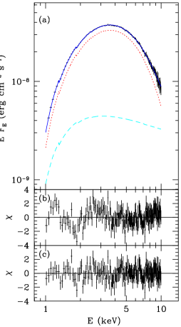
Figure 6: The ASCA/GIS spectrum of GRO J1655–40 and the best-fitting model with $a=0.75$ (see Table 2). Panel $(a)$ shows the data and the model. The model (solid curve) is decomposed into the GR disc (dotted curve) and the power law (dashed curve). The residuals (data–model divided by errors) shown in panel $(c)$ correspond to this fit. For comparison, on panel $(b)$ we present the residuals of the fit without absorption edge.

Finally, our best-fitting model consists of the GR disc, the power law, the interstellar absorption and the absorption edge. Fit results for five values of the black hole spin are presented in Table 2. The data and the best-fitting model for $a=0.75$ are shown on Figure 6.

Table 2: Fit results of the GR disc plus power law and an absorption edge model to GRO J1655–40 ASCA/GIS data for five different values of the black hole spin. The inclination angle is $i=70^{\circ}$ and the distance to the source $D$ = 3.2 kpc. The power-law photon index is fixed at $\Gamma=2.4$. The disc extends from $r_{\rm in}=r_{\rm ms}$ to $r_{\rm out}=10^{4}$. The disc model is described in Section 2.

$a$	0.00	0.25	0.50	0.75	0.998
$N_{\rm H}$ ($10^{21}$ cm-2)	$7.48_{-0.18}^{+0.17}$	$7.48_{-0.17}^{+0.17}$	$7.50_{-0.18}^{+0.17}$	$7.58_{-0.18}^{+0.16}$	$7.70_{-0.17}^{+0.15}$
$E_{\rm edge}$ (keV)	$1.25_{-0.05}^{+0.05}$	$1.25_{-0.05}^{+0.05}$	$1.25_{-0.05}^{+0.05}$	$1.25_{-0.05}^{+0.04}$	$1.23_{-0.04}^{+0.04}$
$\tau_{\rm edge}$	$0.13_{-0.04}^{+0.03}$	$0.13_{-0.03}^{+0.04}$	$0.14_{-0.03}^{+0.04}$	$0.16_{-0.03}^{+0.04}$	$0.17_{-0.03}^{+0.03}$
$M$ (M⊙)	$2.65_{-0.02}^{+0.03}$	$3.19_{-0.03}^{+0.03}$	$4.07_{-0.04}^{+0.04}$	$5.84_{-0.05}^{+0.06}$	$16.2_{-0.2}^{+0.1}$
$\dot{M}_{\rm d}$ ($10^{18}$ g s-1)	3.21${}_{-0.03}^{+0.04}$	2.71${}_{-0.04}^{+0.04}$	2.15${}_{-0.02}^{+0.03}$	1.51${}_{-0.02}^{+0.02}$	0.560${}_{-0.007}^{+0.007}$
$\chi^{2}$/185 d.o.f.	166.1	165.3	164.3	163.4	165.0

Table 3: The same as in Table 2, but now $r_{\rm in}$ is a free fit parameter. For the sake of clarity, we show only $r_{\rm in}$ and $M$.

$a$	0.00	0.25	0.50	0.75	0.998
$r_{\rm in}$	$7.6_{-1.6}^{+12}$	$6.6_{-1.4}^{+9.0}$	$5.5_{-1.3}^{+6.1}$	$3.8_{-0.6}^{+4.7}$	$3.7_{-2.5}^{+4.4}$
$M$ (M⊙)	$2.7_{-1.1}^{+0.0}$	$3.2_{-0.4}^{+0.0}$	$4.0_{-1.4}^{+0.1}$	$5.9_{-1.9}^{+0.0}$	$10_{-6.4}^{+6.3}$
$\chi^{2}$/184 d.o.f.	165.7	165.0	164.1	163.2	163.7

As it was in the case of LMC X-1, spectral fits do not constrain the black hole spin. However, the spin can be constrained taking into account mass limitations. Only the fit with $a=0.75$, yielding $M=5.84_{-0.05}^{+0.06}$M_⊙, is consistent with the mass constraint of (5.5–7.9)M_⊙, inferred from the optical observations by Shahbaz et al. (1999). Again, we fit the data in a range of inclination angles and compute 90 per cent confidential contours for inclination-mass relation. The result is presented on Figure 7. Due to better quality of the data and due to the fact that GRO J1655–40 spectrum is dominated by the disc emission, these contours are much narrower than in the case of LMC X-1. Only the $a=0.75$ contour overlaps with the shaded area indicating allowable values of the inclination angle and the mass. More precise limits on the spin can be found by interpolating between the values found from the fits. If the GR effects are neglected, for the given spectrum the disc must keep constant inner radius while varying $M$ and $a$. Providing that $r_{\rm in}=r_{\rm ms}$, this leads to a simple relation between the mass and the spin $M\propto r_{\rm ms}^{-1}(a)$, where $r_{\rm ms}(a)$ is given by equation (3). The GR effects modify this relation and we have found that a function $M=C_{1}+C_{2}r_{\rm ms}^{-1}(a)$ approximates the data well, so we use it for interpolation. Taking into account uncertainties in the distance to the source, we have found that for given limits $5.5\leq M/$M${}_{\odot}\leq 7.9$ and $64^{\circ}\leq i\leq 71^{\circ}$ the black hole spin is $0.68\leq a\leq 0.88$. In this range of spin values returning radiation is negligible (see Section 2), and does not affect our result.

Figure 7: Black hole mass versus cosine inclination angle for GRO J1655–40. Curves represent 90 per cent confidence contours for fits of the GR disc plus power law model. Distance of $D$ = 3.2 kpc has been assumed. Numbers below contour lines denote the black hole spin. The shaded area corresponds to mass and inclination angle constraints from optical observations (Section 3.2.1).

Next, we fit the data allowing the inner disc radius, $r_{\rm in}$, to be a free parameter. The results are presented in Table 3. In all fits we find that the inner disc radius is consistent with $r_{\rm ms}$, however larger values are possible. Now the $a=0.998$ fit became acceptable with $M=10_{-6.4}^{+6.3}$M_⊙. Since the upper limits for the mass remained virtually the same after freeing $r_{\rm in}$ (see Tables 2 and 3), the lower limit on the spin also remained the same, $a\geq 0.68$, this time.

Within the acceptable range of $M$, $D$ and $i$ (assuming $r_{\rm in}=r_{\rm ms}$) the relative accretion rate, $\dot{m}_{\rm d}$, is between $\sim$ 0.6 and $\sim$ 1.9. In terms of the radiated power it corresponds to a fraction $\eta\dot{m}_{\rm d}\sim$ 0.1–0.2 of the Eddington luminosity. The unabsorbed bolometric luminosity of the disc in GRO J1655–40, computed from the model, is $(1.2$–$1.6)\times 10^{38}$ erg s^-1 ($1.4\times 10^{38}$ erg s^-1 at $D=3.2$ kpc). In the observed energy range only a small fraction of the luminosity is radiated in the tail.

4 Discussion and conclusions

4.1 Black hole mass and spin

Optical and UV observations of black hole binaries can provide with the mass function, which in turn can help estimating, to some extent, the black hole mass and the inclination angle of the binary. We know about a dozen of X-ray Galactic binaries for which the mass function implies the compact object mass larger than 3M_⊙, making them good candidates for black holes. However, the black hole spin cannot be estimated this way.

In this paper we have shown an application of the GR disc model to the soft state X-ray spectra of LMC X-1 and GRO J1655–40 and demonstrated how it can restrict the black hole spin. The model depends on five basic parameters: the black hole mass and spin, the disc inclination angle, the accretion rate and the inner disc radius. Generally, the spectral shape changes only slightly with these parameters, and only two out of them can be established uniquely by fitting the observational data. Additional assumptions about some of the parameters are necessary. In most of our fits we have fixed $i$ and assumed $r_{\rm in}=r_{\rm ms}$. Then, for several fixed values of $a$ we have successfully fitted $M$ and $\dot{M}$. Results presented in Tables 1 and 2 show that $\chi^{2}$ remained virtually the same through the whole range of $a$ and the black hole spin cannot be reckoned this way. On the other hand, at a given spectral shape there is strong correlation between the parameters, in particular between $M$ and $a$ when $i$ and $r_{\rm in}$ are fixed. With an independent estimation of the mass and the inclination angle, we can constrain the black hole spin. The tighter constraints on the mass and the inclination, the more accurate spin estimation can be obtained.

The mass and the inclination angle of LMC X-1 are evaluated rather poorly. Therefore, it is not possible to give a good constrain on the black hole spin. We can only rule out a black hole which is close to, or maximally rotating. GRO J1655–40 gave us better chance. The mass and the inclination angle are measured with relatively high accuracy. Also, due to better quality of the X-ray data, we have obtained smaller statistical errors on $M$. As a result, we could limit the spin, $0.68\leq a\leq 0.88$ (when $r_{\rm in}=r_{\rm ms}$). This result is only weakly affected by neglecting returning photons, which are negligible for spin less then 0.9.

We underline, that when we allow for free $r_{\rm in}>r_{\rm ms}$, no upper limit for the black hole spin can be imposed. This is because for a given spectral shape increase of $r_{\rm in}$ with fixed $M$ and $i$ leads to increase of $a$. However, there are clues that the accretion disc in BHB extends down to the marginally stable orbit all the time in the soft (high or very high) state.

Long-term 1996-1997 RXTE monitoring of GRO J1655–40 (Sobczak et al. 1999) shows remarkable constancy of the MCD inner disc radius over the period of a few hundred days, while the source went through the high and very high spectral states. There is an exception of a few observations during the very high state, where the inner radius dropped suddenly by factor $\sim 3$. Merloni, Fabian & Ross (2000) interpret it as a drop in the disc accretion rate, which caused increase of the hardening factor and decrease of the apparent inner radius, while the actual $r_{\rm in}$ has not changed. If the inner disc radius remained constant indeed, it is reasonable to assume that the disc extended down to the marginally stable orbit all the time when the source was in the high or very high state, including also the ASCA observation analysed in this paper.

Long-term 1996-1998 RXTE monitoring of LMC X-1 (Wilms et al. 2001) shows in turn significant variations of the MCD inner disc radius. However, it is not clear whether these variations can be attributed to real changes of $r_{\rm in}$. They might be, at least in part, due to systematic errors in the model.

So, does $r_{\rm in}$ vary during the soft state or not? If the cold disc in either of the above observations was indeed truncated, it should turn into an optically thin inner flow below $r_{\rm in}$. Hot plasma in the inner flow could be a source of the high-energy tail beyond the disc spectrum. However, optically thin solution can exist only for luminosities lower than a few per cent of the Eddington luminosity. At higher accretion rates (and higher densities) Coulomb transfer of energy from the protons to the electrons becomes efficient, the optically thin flow becomes radiatively efficient and collapses to the optically thick Shakura-Sunyaev disc (Chen et al. 1995; Esin, McClintock & Narayan 1997). In both observations analysed in this paper luminosity exceeded 10 per cent of $L_{\rm Edd}$, therefore we should not expect any hot, optically thin flow. Instead, we propose that the cold disc extends all the way down to the marginally stable orbit, and the high-energy tail emission is produced in active regions above the disc. Hence, we find the assumption of $r_{\rm in}=r_{\rm ms}$ as well founded, and our best constraint on the black hole spin in GRO J1655–40 is $0.68\leq a\leq 0.88$ and in LMC X-1 we rule a black hole rotating with the spin close to maximum.

The most spectacular feature of GRO J1655–40 is its radio jets (Tingay et al. 1995; Hjellming & Rupen 1995), observed also in another high-spin black hole candidate, GRS 1915+105 (Mirabel & Rodríguez 1994). Co-existence of relativistic jets and rotating black holes in BHB makes and interesting link to the problem of radio dichotomy of quasars, and supports the black hole “spin paradigm”, according to which jets in quasars are powered by rotating black holes (e.g. Moderski, Sikora & Lasota 1998). Since no strong radio jets were found in LMC X-1, the non-rotating black hole should be expected in this system. Unfortunately, our results do not allow us to make such claims. Further systematic studies of several jet and non-jet sources could provide with more evidences for the spin paradigm.

4.2 Compton reflection

The X-ray spectra of LMC X-1 and GRO J1655–40 are similar to the soft state spectrum of Cyg X-1 (Gierliński et al. 1999), though the first two sources are significantly brighter. An important difference is that we do not find Compton reflection features here, while Cyg X-1 in the soft state showed strong reflection component with covering angle $\Omega/2\pi\sim 0.7$ and a broad Fe K$\alpha$ line. This can be explained by the instrumental limitations or/and by the intrinsic difference in the source geometry and energetics. The Compton reflection from the cold matter can be identified by Fe K$\alpha$ features around 7 keV and by reflection continuum, which peaks around 30 keV in the $EF_{E}$ spectrum. Since ASCA can observe only up to $\sim$ 10 keV, the detection of the reflection continuum with ASCA data only might be difficult, if not impossible. The iron K edge and line parameters are sensitive to the shape of the underlying continuum, which cannot be properly established without the high-energy data. For example, Dotani et al. (1997) analysed the ASCA data of Cyg X-1 and did not find any Fe line. Gierliński et al. (1999) re-analysed the same data jointly with the simultaneous RXTE observation, and found the presence of the iron line with high statistical significance. LMC X-1 spectrum has poor statistics above $\sim$ 5 keV, so the reflection features can escape the detection. The high-energy tail in GRO J1655–40 is much weaker than in Cyg X-1. At 7 keV the disc radiates $\sim 3.5$ times more energy than the tail. Therefore, the Fe K-shell features will be very weak in the total spectrum, and difficult to detect. In the soft state of Cyg X-1 the situation is opposite: the disc emission at 7 keV is negligible (see Figure 8 in Gierliński et al. 1999 and Figure 4 in this paper). Moreover, the Fe K-shell features coming from the disc around the fast-spinning black hole are significantly smeared, which additionally hinders the detection.

We note, that ASCA and RXTE detected characteristic iron features in GRO J1655–40, at different periods (Ueda et al. 1998; Tomsick et al. 1999; Bałucińska-Church & Church 2000; Yamaoka et al. 2000). However, precise ASCA/RXTE observations show that these features can be consistently explained by resonant absorption lines in the corona above the disc without reflection components (Yamaoka et al. 2000).

4.3 Disc stability

An unclear issue is stability of the cold disc. Both sources are very bright with luminosities being a significant fraction of the Eddington luminosity ($\dot{m}_{\rm d}\sim$ 1–5 is a very conservative limit for LMC X-1). A radiation pressure dominated region, which is thought to be unstable, arises in the disc above the critical accretion rate, $\dot{m}_{\rm crit}$. In the pseudo-Newtonian approximation, for a 10M_⊙ black hole and $\alpha=0.1$, $\dot{m}_{\rm crit}\approx 0.64$ (Gierliński et al. 1999; taking into account accretion in the cold disc only, i.e. $f=0$). Therefore, the discs in both sources seem to be dominated by the radiation pressure. Since we consider here rotating black holes, we checked this result by calculating the ratio of the radiation pressure to the gas pressure in the Kerr metric (Novikov & Thorne 1972), for all acceptable fit parameters in Tables 1 and 2. We found that in both sources the inner part of the cold accretion disc below several tens of $R_{g}$ is dominated by the radiation pressure indeed. Thus, both discs should be unstable against secular and thermal instabilities. However, despite this inconvenience the discs in LMC X-1 and GRO J1655–40 apparently do exist.

This riddle probably arises from our lack of understanding of microscopic mechanisms of accretion. The instability develops in the standard $\alpha$-prescription theory, where $r\phi$-element of the viscous stress tensor, $T_{r\phi}$, is proportional to the total pressure, i.e. to the sum of the gas pressure and the radiation pressure. The viscosity parameter $\alpha$ includes not well understood physics of viscosity, which is supposed to be due to chaotic magnetic fields and turbulence in the gas flow. It is not quite clear why $T_{r\phi}$ should be proportional to the total pressure. If we assume that $T_{r\phi}$ is proportional to the gas pressure only (the so-called $\beta$-disc; see e.g. Stella & Rosner 1984), the disc becomes stable in the radiation pressure dominated region (Figure 8). The existence of the radiation pressure dominated discs should impose significant constraints on the theoretical models of viscosity in the accretion flow.

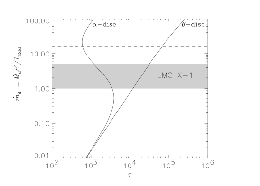
Figure 8: Two solutions of the optically thick disc around a 10M_⊙ non-rotating black hole at the radius of the most significant instability of $r$ = 15.1. The viscosity parameter $\alpha$ is 0.1. The left-hand curve represents the solution with $T_{r\phi}\propto P_{\rm rad}+P_{\rm gas}$ ($\alpha$-disc). The right-hand curve shows the solution with $T_{r\phi}\propto P_{\rm gas}$ ($\beta$-disc). The shaded region shows the most conservative limits on the disc accretion rate of LMC X-1 at $a=0$. The dashed line represents the Eddington luminosity (efficiency $\eta=1/16$). The inner disc is dominated by the radiation pressure, where the $\alpha$-disc solution is unstable and the $\beta$-disc solution is stable.

4.4 Model reliability

One important question we should ask is reliability of the model and parameters inferred. While modelling the disc spectrum in the “proper” way one should solve the following four problems. (i) The radial disc structure, (ii) the vertical disc structure, (iii) the radiation transfer and (iv) the relativistic effects. Our understanding of the first three problems is poor and there are still a lot of open questions concerning the viscosity prescription, vertical distribution of gravitational energy dissipation, effects of radiation pressure and irradiation of the disc, importance of bound-free opacity and heavy elements, and importance of Comptonization, just to name the most important issues. Consequently, every single prediction available in the literature is based on simplifying assumptions and is model dependent. On the other hand, the simplest solution, i.e. the sum of blackbodies gives the best description of the observational data. For example, a smooth multicolour spectrum with no ionization edges consistently reproduces the AGN observations in which the Lyman edge (expected by more advanced models) is not observed. As we have shown in this chapter, the multicolour model fits the black hole candidate spectra perfectly as well.

We correct the emerging spectra for two effects that significantly affect measurements of the disc normalization and temperature. The first one is a deep gravitational potential in the vicinity of a fast rotating black hole. All special and general relativistic effects are treated to high accuracy by means of the transfer function, as was described in Section 2. The second important aspect is the effect of electron scattering, which we approximate by a single colour temperature correction factor, $f_{\rm col}$, using a diluted blackbody as a local spectrum (see Section 2). Under certain simplifying assumptions Shimura & Takahara (1995) computed the vertical disc structure around a Schwarzschild stellar-mass black hole and solved the radiation transfer. They found that for the viscosity parameter $\alpha=0.1$ the local spectrum can be represented by a diluted blackbody when Comptonization is effective, which takes place in the inner disc region when $\dot{m}_{\rm d}\ga 1$. For $M=10$M_⊙ and $\dot{m}_{\rm d}=1$ they found that the sum of diluted blackbodies fits the whole disc spectrum very well with the best-fitting hardening factor of $f_{\rm col}=1.7$ (see Figure 2 in Shimura & Takahra 1995). Merloni et al. (2000) made a similar comparison between the multicolour disc and a more realistic disc model with the vertical temperature structure and radiation transfer solved and came up with a comparable result. The multicolour disc spectra fit the realistic disc spectra well, and for $\dot{m}_{\rm d}\ga 1$ the hardening factor is $f_{\rm col}\approx 1.8$. In both observations in this paper $\dot{m}_{\rm d}\sim 1$, therefore, within the trustworthiness limits of the Shimura & Takahara and Merloni et al. calculations, we find our model reliable. A small variation in the hardening factor does not change our results significantly. For example, the GRO J1655–40 spin for $f_{\rm col}=1.8$ is $0.60\leq a\leq 0.83$.

Appendix A Construction of the photon transfer function

We consider a gravitational field of a rotating black hole with the mass $M$, and the angular momentum, $J$. In both appendices we use $G=c=1$ units, the $(-+++)$ signature and the Boyer-Lindquist coordinates, $(t,R,\theta,\phi)$. Non-zero components of the metric tensor are given by

$$g_{tt} = -(1-2r/\Sigma),$$

$$g_{t\phi} = -2ar\sin^{2}\theta/\Sigma,$$

$$g_{\phi\phi} = \left(r^{2}+a^{2}+{2a^{2}r\sin^{2}\theta\over\Sigma}\right)\sin^{2}\theta,$$

$$g_{rr} = \Sigma/\Delta,$$

$$g_{\theta\theta} = \Sigma,$$ (11)

where

$$\Delta=r^{2}+a^{2}-2r,$$

$$\Sigma=r^{2}+a^{2}\cos^{2}\theta,$$ (12)

and we use dimensionless distance and specific angular momentum parameter

$$r={R\over M},~{}~{}~{}~{}a={J\over M^{2}}.$$ (13)

Our approach to calculation of the disc photon trajectories mostly follows that of Cunningham (1975). A null geodesic in the Kerr metric is described by two constants of motion, $\lambda$ and $\xi$, defined as

$$\lambda={L\over EM},~{}~{}~{}~{}\xi^{2}={C\over E^{2}M^{2}},$$ (14)

where $E$ is the photon energy at infinity, $L$ is projection of the photon angular momentum on the symmetry axis and $C$ is the Carter constant (in the definition of $\xi$ we took into account the condition $C\geq 0$ satisfied by trajectories intersecting equatorial plane.)

We take an usual assumption that the radial velocity in the disc can be neglected and its motion is Keplerian. In the non-rotating frame, the angular velocity and the linear velocity, respectively, are given by

$$\Omega_{\rm K}={1\over M}{1\over r^{3/2}+a},$$ (15)

and

$$V_{\rm K}={A\over r^{2}\sqrt{\Delta}}\left(\omega_{\rm K}-{2ar\over A}\right),$$ (16)

where

$$A=r^{4}+a^{2}r^{2}+2a^{2}r,$$ (17)

and $\omega_{\rm K}=M\Omega_{\rm K}$. Then, we get the following relation between the constants of motion and the emission angles in the disc rest frame (e.g., Cunningham & Bardeen 1973)

$$\lambda = {\sin\theta_{e}\sin\phi_{e}+V_{\rm K}\over(r_{e}^{2}\Delta^{1/2}+2ar_{e}V_{\rm K})/A+\omega_{\rm K}\sin\theta_{e}\sin\phi_{e}},$$

$$\xi = \left({A\over\Delta}\right)^{1/2}(1-V_{\rm K}^{2})^{-1/2}(1-\lambda\omega_{\rm K})\cos\theta_{e}.$$ (18)

where $r_{e}$ is the initial photon radius, $\theta_{e}$ is a polar angle between the photon initial direction and the normal to the disc and $\phi_{e}$ is the azimuthal angle, in the disc plane, with respect to the $r$-direction.

Then, the redshift of the photon emitted from the disc at a distance $r_{e}$ is given by

$$g_{\rm eff}=r_{e}\left({\Delta\over A}\right)^{1/2}{(1-V_{\rm K}^{2})^{1/2}\over 1-\omega_{\rm K}\lambda},$$ (19)

and the angle, $i$, at which the photon will be observed far from the disc in the flat space-time is determined by the integral equation of motion

$$\pm\int_{r_{e}}^{\infty}\Re^{-1/2}{\rm d}r=\int_{\pi/2}^{i}\Theta^{-1/2}{\rm d}\theta.$$ (20)

where $\Re$ and $\Theta$ are radial and polar effective potentials, respectively,

$$\Re(r)=(r^{2}+a^{2}-\lambda a)^{2}-\Delta\left[\xi^{2}+(\lambda-a)^{2}\right],$$

$$\Theta(\theta)=\xi^{2}+\cos^{2}\theta\left(a^{2}-\lambda^{2}/{\sin^{2}\theta}\right).$$ (21)

The photon transfer function is tabulated in discrete steps in five dimensions ($a$, $r_{e}$, $\cos i$, $g_{\rm eff}$, $\cos\theta_{e}$). Generated photons are summed in the appropriate elements of the photon transfer function table according to the following algorithm.

1. for given $a$ and $r_{e}$ generate the photon initial direction from the distribution uniform both in $\phi_{e}$ and $\cos\theta_{e}$,

2. find the constants of motion from equation (18),

3. solve equation (20) for $i$ (initial sign of $\Re$ in equation (20) is negative for $\pi/2<\phi_{e}<3\pi/2$ and positive otherwise),

4. find $g_{\rm eff}$ from equation (19),

5. increment an element of the transfer function table corresponding to $a$, $r_{e}$, $\cos i$, $g_{\rm eff}$ and $\cos\theta_{e}$.

In order to compute and tabulate the transfer function we have calculated trajectories of $10^{9}$ photons. The disc is axially symmetric and emission from a given point of the disc is also axially symmetric. Therefore, integration over $\phi_{e}$ for trajectories starting at a given point of the disc and observed at a given angle $i$ and collected at all angles $\phi_{o}$ is equivalent to integration over all trajectories starting at a given radius $r_{e}$, which are observed at a given angle $i$ and any particular $\phi_{o}$.

Appendix B Transformation of the photon number intensity

As pointed out in Section 2, application of the photon transfer function requires transformation of the photon number intensity between the reference frames of the distant observer (the Boyer-Lindquist coordinate frame) and the observer co-rotating with the disc. The latter one is represented by the covariant tetrad (we show only the components used below):

$$e^{t^{\prime}}=-r^{-1}\left(1-V_{\rm K}^{2}\right)^{-1/2}\left({A\over\Delta}\right)^{1/2}$$

$$~{}~{}~{}~{}\times\left(g_{tt}+\omega_{\rm K}g_{t\phi},0,0,g_{t\phi}+\omega_{\rm K}g_{\phi\phi}\right),$$

$$e^{r^{\prime}}=(0,r/\sqrt{\Delta},0,0),$$

$$e^{\phi^{\prime}}=r^{-1}\left(1-V_{\rm K}^{2}\right)^{-1/2}\left({A\over\Delta}\right)^{1/2}\left[V_{\rm K}g_{tt}+g_{t\phi}\left({r^{2}\Delta^{1/2}\over A}\right.\right.$$

$$~{}~{}~{}~{}\left.\left.+{2arV_{\rm K}\over A}\right),0,0,V_{\rm K}g_{t\phi}+g_{\phi\phi}\left({r^{2}\Delta^{1/2}\over A}+{2arV_{\rm K}\over A}\right)\right],$$ (22)

where order of vector components is given by $(t,r,\theta,\phi)$, and primes denote coordinates defined in the disc local rest frame. Then, the one-form ${\rm d}t^{\prime}$ can be written in terms of the Boyer-Lindquist coordinates as

$${\rm d}t^{\prime}=e_{t}^{t^{\prime}}{\rm d}t+e_{\phi}^{t^{\prime}}{\rm d}\phi$$ (23)

As for the observer at rest in the disc ${\rm d}\phi^{\prime}=0$, and

$${\rm d}\phi^{\prime}=e_{t}^{\phi^{\prime}}{\rm d}t+e_{\phi}^{\phi^{\prime}}{\rm d}\phi,$$ (24)

we obtain the following relation

$${\rm d}t^{\prime}=\beta_{t}{\rm d}t,$$ (25)

where

$$\beta_{t}=e_{t}^{t^{\prime}}-e_{\phi}^{t^{\prime}}e_{t}^{\phi^{\prime}}/e_{\phi}^{\phi^{\prime}}.$$ (26)

Similarly, for the disc unit area we find

$${\rm d}r^{\prime}{\rm d}\phi^{\prime}=e_{r}^{r^{\prime}}{\rm d}r\left(e_{t}^{\phi^{\prime}}{\rm d}t+e_{\phi}^{\phi^{\prime}}{\rm d}\phi\right)=\beta_{S}{\rm d}r{\rm d}\phi$$ (27)

(in the latter equality we have used the condition ${\rm d}t^{\prime}=0$, relevant for the three-space measurements in the disc rest frame), where

$$\beta_{S}=e_{r}^{r^{\prime}}\left(e_{\phi}^{\phi^{\prime}}-e_{\phi}^{t^{\prime}}e_{t}^{\phi^{\prime}}/e_{t}^{t^{\prime}}\right).$$ (28)

The factor $\beta_{S}$ gives correction for the integral element ${\rm d}r{\rm d}\phi$ in equation (1) (integration over $\phi$ is hidden in the convolution) which should be taken into account in calculation of the number of photons emitted from the accretion disc.

References

- [] Anders E., Grevesse N., 1989, Geochim. Cosmochim. Acta, 53, 197
- [] Arnaud K. A., 1996, in Jacoby G. H., Barnes J., eds., Astronomical Data Analysis Software and Systems V. ASP Conf. Series Vol. 101, San Francisco, p. 17
- [] Asaoka I., 1989, PASJ, 41, 763
- [] Bailyn C. D., et al., 1995a, Nature, 374, 701
- [] Bailyn C. D., Orosz J. A., McClintock J. E., Remillard R. A., 1995b, Nature, 378, 157
- [] Bałucińska-Church M., McCammon D., 1992, ApJ, 400, 699
- [] Bałucińska-Church M., Church M. J., 2000, MNRAS, 312, L55
- [] Chen X., Abramowicz M., Lasota J.-P., Narayan R., Yi I., 1995, ApJ, 443, 61L
- [] Cowley A. P., Schmidtke P. C., Anderson A. L., McGrath T. K., 1995, PASP, 107, 145
- [] Cui W., Zhang S. N., Chen W., 1997, ApJ, 492, L53
- [] Cunningham C. T.: 1975, ApJ, 202, 788
- [] Cunningham C. T.: 1976, ApJ, 208, 534
- [] Cunningham C. T., Bardeen J. M., 1973, ApJ, 183, 237
- [] Dotani T. et al., 1997, ApJ, 485, L87
- [] Ebisawa K., 1991, Ph.D. Thesis
- [] Ebisawa K., Mitsuda K., Inoue H., 1989, PASP, 41, 519
- [] Ebisawa K., Mitsuda K., Hanawa T., 1991, ApJ, 367, 213
- [] Ebisawa K., Makino F., Mitsuda K., Belloni T., Cowley A. P., Schmidtke P. C., Treves A., 1993, ApJ, 403, 684
- [] Ebisawa K., et al., 1994, PASJ, 46, 375
- [] Esin A. A., McClintock J. E., Narayan R., 1997, ApJ, 489, 865
- [] Feast M. W., Catchpole R. M., 1997, MNRAS, 286, L1
- [] Fu A., Taam R. E., 1990, ApJ, 349, 553
- [] Gierliński M., Zdziarski A. A., Done C., Johnson W. N., Ebisawa K., Ueda Y., Haard F., Phlips B. F., 1997, MNRAS, 288, 958
- [] Gierliński M., Zdziarski A. A., Poutanen J., Coppi P. S., Ebisawa K., Johnson W. N., 1999, MNRAS, 309, 496
- [] Grove J. E., Johnson W. N., Kroeger R. A., McNaron-Brown K., Skibo J. G. Phlips B. F., 1998, ApJ, 500, 899
- [] Gruzinov A., 1999, astro-ph/9910335
- [] Hanawa T., 1989, ApJ, 341, 948
- [] Hjellming R. M., Rupen M. P., 1995, Nature, 375, 464
- [] Hutchings J. B., Crampton D., Cowley A. P., Bianchi L., Thompson I. B., 1987, AJ, 94, 340
- [] Laor A., 1990, MNRAS, 246, 369
- [] Laor A., Netzer H., Piran T., 1990, MNRAS, 242, 560
- [] Makishima K., et al., 2000, ApJ, 535, 632
- [] Merloni A., Fabian A. C., Ross R. R., 2000, MNRAS, 313, 193
- [] Mirabel I. F., Rodríguez L. F., 1994, Nature, 371, 46
- [] Mitsuda K. et al., 1984, PASJ, 36, 741
- [] Moderski R., Sikora M., Lasota J.-P., 1998, MNRAS, 301, 142
- [] Novikov I. D., Thorne K. S., 1972, in: DeWitt C., DeWitt B. S., Black holes, Gordon and Beach Science Publishers, p. 343
- [] Nowak M. A., Wilms J., Heindl W. A., Pottschmidt K., Dove J. B., Begelman M. C., 2001, MNRAS, 320, 316
- [] Orosz J.A., Bailyn, C.D.: 1997, ApJ, 477, 876
- [] Page D. N., Thorne K. S.: 1974, ApJ, 191, 499
- [] Phillip K. C., Mészáros P.: 1986, ApJ, 310, 284
- [] Press W. H., Teukolsky S. A., Vetterling W. T., Flannery B. P., 1992, Numerical Recipes. Cambridge Univ. Press, Cambridge
- [] Remillard R. A., Morgan E. H., McClintock J. E., Bailyn C. D., Orosz J. A., 1999, ApJ, 522, 397
- [] Schlegel E. M., Marshall F. E., Mushotzky R. F., Smale A. P., Weaver K. A., Serlemitsos P. J., Petre R., Jahoda K. M., 1994, ApJ, 422, 243
- [] Schmidtke P. C., Ponder A. L., Cowley A. P., 1999, ApJ, 117, 1292
- [] Shakura N. I., Sunyaev R. A., 1973, A&A, 24, 337
- [] Shahbaz T., van der Hooft F., Casares J., Charles P. A., van Paradijs J., 1999, MNRAS, 306, 89
- [] Shimura T., Takahara F.: 1995, ApJ, 445, 780
- [] Sobczak G. J., McClintock J. E., Remillard R. A., Bailyn C. D., Orosz J. A., 1999, ApJ, 520, 776
- [] Stanek K. Z., Zaritsky D., Harris J., 1998, ApJ, 500, L141
- [] Stella L., Rosner R., 1984, ApJ, 277, 312
- [] Stella L., Vietri M., Morsink S. M., 1999, ApJ, 524, L63
- [] Tavani M., Fruchter A., Zhang S. N., Harmon B. A., Hjellming R. N., Rupen M. P., Bailyn C., Livio M., 1996, ApJ, 473, L103
- [] Thorne K. S., 1974, ApJ, 191, 507
- [] Tingay S. J., et al., 1995, Nature, 374, 141
- [] Tomsick J. A., Kaaret P., Kroeger R. A., Remillard R. A., 1999, ApJ, 512, 892
- [] Treves A., et al., 2000, Advances in Space Res., 25, 437
- [] Ueda Y., Inoue, H., Tanaka, Y., Ebisawa, K., Nagase, F., Kotani, T., Gehrels, N.: 1998, ApJ, 492, 782
- [] van der Hooft F., Heemskerk M. H. M., Alberts F., van Paradijs J., 1998, A&A, 329, 538
- [] Wilms J., Nowak M. A., Pottschmidt K., Heindl W. A., Dove J. B., Begelman M. C., 2001, MNRAS, 320, 327
- [] Yamada T. T., Mineshige S., Ross R. R., Fukue J., 1994, PASJ, 46, 553
- [] Yamaoka K., Ueda Y., Inoue H., Nagase F., Ebisawa K., Kotani T., Tanaka Y., Zhang S. N., 2000, ApJ, submitted
- [] Zdziarski A. A., Johnson W. N., Magdziarz P., 1996, MNRAS, 283, 193
- [] Zdziarski A. A., Poutanen J., Mikołajewska J., Gierliński M., Ebisawa K., Johnson W. N., 1998, MNRAS, 301, 435
- [] Zhang S. N., Wilson C. A., Harmon B. A., Fishman G. J., Wilson R. B., Paciesas W. S., Scott M., Rubin B. C., 1994, IAU Circ. 6046
- [] Zhang S. N., Cui W., Chen W., 1997a, ApJ, 482, L155
- [] Zhang S. N., et al., 1997b, ApJ, 479, 381