Origin of quasi–periodic shells in dust forming AGB winds

We have combined time dependent hydrodynamics with a two–fluid model for dust driven AGB winds. Our calculations include self–consistent gas chemistry, grain formation and growth, and a new implementation of the viscous momentum transfer between grains and gas. This allows us to perform calculations in which no assumptions about the completeness of momentum coupling are made. We derive new expressions to treat time dependent and non–equilibrium drift in a hydro code. Using a stationary state calculation for IRC +10216 as initial model, the time dependent integration leads to a quasi–periodic mass loss in the case where dust drift is taken into account. The time scale of the variation is of the order of a few hundred years, which corresponds to the time scale needed to explain the shell structure of the envelope of IRC +10216 and other AGB and post-AGB stars, which has been a puzzle since its discovery. No such periodicity is observed in comparison models without drift between dust and gas.

1 Introduction

Dust driven winds are powered by a fascinating interplay of radiation, chemical reactions, stellar pulsations and dynamics. As soon as the envelope of a star on the Asymptotic Giant Branch (AGB) develops sites suitable for the formation of solid “dust” (i.e. sites with a relatively high density and a low temperature) its dynamics will be dominated by radiation pressure. Dust grains are extremely sensitive to the stellar radiation and experience a large radiation pressure. The acquired momentum is partially transferred to the ambient gas by frequent collisions. The gas is then blown outward in a dense, slow wind that can reach high mass loss rates.
The detailed observations of (post) AGB objects and Planetary Nebulae (PN) that have become available during the last decade have shown that winds from late type stars are far from being smooth. The shell structures found around e.g. CRL 2688 (the “Egg Nebula”, Ney et al. (1975); Sahai et al. (1998)), NGC 6543 (the Cat’s Eye Nebula, Harrington & Borkowski (1994)) and the AGB star IRC +10216 (Mauron & Huggins 1999, 2000), indicate that the outflow has quasi–periodic oscillations. The time scale for these oscillations is typically a few hundred years, i.e. too long to be a result of stellar pulsation, which has a period of a few hundred days, and too short to be due to nuclear thermal pulses, which occur once in ten thousand to hundred thousand years.
Stationary models, in which gas and dust move outward as a single fluid, do not suffice to explain the observations. Instead, time dependent two–fluid hydrodynamics, preferably including (grain) chemistry and radiative transfer, may help to explain the origin of these circumstellar structures.
Time dependent hydrodynamics has been used to study the influence of stellar pulsations on the outflow (Bowen (1988); Fleischer et al. (1992)). The coupled system of radiation hydrodynamics and time dependent dust formation was solved by Höfner et al. (1995).
Stationary calculations, focused on a realistic implementation of grain nucleation and growth, have been developed in the Berlin group, initially for carbon–rich objects (Gail et al. (1984); Gail & Sedlmayr (1987)) and more recently also for the more complicated case of silicates in circumstellar shells of M stars (Gail & Sedlmayr (1999)).
Two–fluid models, in which dust and gas are not necessarily co–moving, have been less well studied. Berruyer & Frisch (1983), Berruyer (1991) and MacGregor & Stencel (1992), pointed out that, for stationary and isothermal envelopes, the assumption of complete momentum coupling breaks down at large distances above the photosphere and for small grains. Self–consistent, but again stationary, two–fluid models, considering the grain size distribution, dust formation and the radiation field were developed by Krüger and co–workers (Krüger et al. (1994); Krüger & Sedlmayr (1997)).
The only studies in which time dependent hydrodynamics and two–fluid flow have been combined so far are the work of Mastrodemos et al. (1996) and that of the Potsdam group (Steffen et al. (1997); Steffen et al. (1998); Steffen & Schönberner (2000)).
In the next section, we will argue that time dependence and two–fluid flow are not just two interesting aspects of stellar outflow but that they have to be combined. It turns out that fully free two–fluid flow, i.e. in which no assumptions at all about the amount of momentum transfer between both phases are made, can only be achieved in time dependent calculations. In two–fluid flow, both phases are described by their own continuity and momentum equations. Momentum exchange occurs through viscous drag, i.e. through gas–grain collisions. The collision rate and the momentum exchange per collision depend on the velocity of grains relative to the gas. Hence, by fixing the drag force, one fixes the relative velocity and the system becomes degenerate.
In this paper we present our two–fluid time dependent hydrodynamics code. We have selfconsistently included equilibrium gas chemistry and grain nucleation and growth, see Section 3. In order not to make assumptions on the viscous coupling, we consider, in Section 3.4, the microphysics of gas–grain collisions. Results are given in Section 4.

2 Grain drift and momentum coupling

2.1 Definitions

The acceleration of dust grains, as a result of radiation pressure, leads to an increase in the gas–dust collision rate. The viscous drag force (the rate of momentum transfer from grains to gas due to these collisions) is proportional to the collision rate and to the relative velocity of grains with respect to the gas. This force is discussed in the next section in more detail. The drag force provides a (momentum) coupling between the gaseous and the solid phase.
The gas–dust coupling was studied by e.g. Gilman (1972), who distinguished two types of coupling. Gas and grains are position coupled when the difference in their flow velocities, the drift velocity, is small compared to the gas velocity, i.e. when the grains move slowly through the gas. Momentum coupling, on the other hand, requires that the momentum acquired by the grains through radiation pressure is approximately equal to the momentum transferred from the grains to the gas by collisions. The situation in which both are exactly equal is called full or complete momentum coupling. Gilman (1972) stated that, if both forces are equal, grains drift at the terminal drift velocity. A less confusing term for the same situation was introduced by Dominik (1992): equilibrium drift. The idea is that since the drag force increases with increasing drift velocity, an equilibrium value can be found by equating the radiative acceleration of the grains and the deceleration due to momentum transfer to the gas. Note that, when calculating the equilibrium value of the drift velocity that way, i.e. assuming complete momentum coupling, one implicitly assumes that grains are massless. A physically correct way to calculate the equilibrium drift velocity is to demand gas and grains to have the same acceleration.

2.2 Single and multi–fluid models

Various groups have studied the validity of momentum coupling, with and without assuming equilibrium drift, in stationary and in time dependent calculations. Others have just applied a certain degree of momentum coupling in model calculations carried out to study other aspects of the wind. We will give a brief overview of the most important of these studies, resulting in the conclusion that prior to our attempt, full two–fluid hydrodynamics has been presented only twice. Because the meaning of terms like “full” and “complete” momentum coupling, “terminal” and “equilibrium” drift seem to be slightly different from author to author, we will first give our own definitions for three classes of models.
First, single–fluid models are those in which only the momentum equation of the gas component is solved. All momentum due to radiation pressure on grains is transferred fully and instantaneously to the gas. If, e.g., for the calculation of grain nucleation and growth rates, a value for the flow velocity of the dust component is needed, the dust is just assumed to have the same velocity as the gas: drift is assumed to be negligible. Hence, in terms of Gilman (1972), in single fluid models grains are both position and (completely) momentum coupled to the gas.
The second class is that of the two–fluid models. Here, again in terms of Gilman (1972), grains are not necessarily position and momentum coupled to the gas. Grains can drift at non–equilibrium drift velocities. Hence, grains and gas are neither forced to have equal velocity nor forced to have equal acceleration.
The third category of models represents what we will call 1.5–fluid models. In these models, grains are assumed to drift at the equilibrium drift velocity with respect to the gas. No assumptions about position coupling are made. In other words, gas and grains are equally accelerated but do not necessarily have the same velocity. The equilibrium drift velocity is calculated by equating the drag force and the radiation pressure on the grains, see Dominik (1992), or, more accurately, by demanding gas and grains to be equally accelerated. Only the momentum equation of the gas is solved, the dust velocity is determined by simply adding the gas velocity and the equilibrium drift velocity.

2.3 Stationary models

Although the above classification for modeling methods also applies to stationary models, extra care is needed there. When trying to do two–fluid stationary modeling one should realize that the condition of stationarity itself will also introduce momentum coupling. This can be understood as follows. Equilibrium drift is the state in which gas and grains are equally accelerated:

$$\frac{\mathrm{d}v_{\mathrm{g}}}{\mathrm{d}t}=\frac{\mathrm{d}v_{\mathrm{d}}}{\mathrm{d}t}$$ (1)

The derivative in this equation is a total derivative. Imposing stationarity, the temporal contribution to this total derivative vanishes by definition, and Eq.(1) reduces to

$$v_{\mathrm{g}}\frac{\partial v_{\mathrm{g}}}{\partial r}=v_{\mathrm{d}}\frac{\partial v_{\mathrm{d}}}{\partial r}$$ (2)

The difference between both sides of Eq.(2) can be small, especially in the outer layers of the envelope, where the velocities reach a more or less constant value. Therefore, the occurrence of equilibrium drift in a stationary outflow may be partially due to the condition of stationarity itself. For this reason, one should be very careful when checking the validity of momentum coupling against stationary calculations. Moreover, in order to make a calculation fully self–consistent, no assumptions on momentum coupling should be made. Hence, for fully self–consistent modeling, time dependent calculations are to be preferred.

2.4 Overview of previous modeling

Examples of single fluid calculations are naturally found in studies in which drift and momentum coupling are not the topic of research, e.g. the work of Dorfi & Höfner (1991) and Fleischer et al. (1995). Both perform time dependent hydrodynamics, assuming that the influence of drift on the aspect of the flow under consideration, dust formation and nonlinear effects due to dust opacity, is negligible.
The completeness of momentum coupling is investigated by Berruyer & Frisch (1983) and by Krüger et al. (1994). The former first find a (stationary) wind solution under the assumption of complete momentum coupling, noticing that this assumption causes the two–fluid character to be lost. Next, in order to check the validity of their supposition, they find a stationary solution for the system, including the grain momentum equation. Both calculations give very similar results near the photosphere, from which it is concluded that momentum coupling is complete there. Far away from the stellar surface ($\gtrsim 1000R_{\mathrm{*}}$), the results are different so that momentum coupling is said to be invalid there. We too, find that non–equilibrium drift arises far away from the photosphere (see Section 4). We would like to remark, however, that it may not be sufficient to verify the validity of complete momentum coupling by comparing with stationary calculations, see Section 2.3.
Krüger et al. (1994) undertook a similar study, which is the most realistic stationary two–fluid calculation up to now. It treats the coupled system of hydrodynamics and thermodynamics, but also involves chemistry and dust formation (simplified by the assumption of instantaneous grain formation). Krüger et al. conclude that momentum coupling can be assumed to be complete and therefore disagree with Berruyer & Frisch (1983). We think this may be due to the fact that Krüger et al. run their calculation out to about ten stellar radii, whereas Berruyer & Frisch compute outwards to several thousand stellar radii.
According to MacGregor & Stencel (1992), who use a simple model for grain growth in a stationary, isothermal atmosphere, the assumption of complete momentum coupling appears to break down for grain sizes smaller than about $5\times 10^{-6}$ cm.
Prior to our attempt, time dependent two–fluid hydrodynamics was presented by Mastrodemos et al. (1996). They conclude that fluctuations on the time scale of the variability periods of Miras and LPV (Long Period Variables), 200-2000 days, can not persist in the wind. Since they do not calculate grain nucleation and growth self–consistently but instead assume that grains grow instantaneously and have a fixed size, the extreme non–linear coupling between shell dynamics, chemistry and radiative transfer (cf. Sedlmayr (1997)) is not present. Our calculations however indicate that this chemo–dynamical coupling is a main ingredient to the occurence of variability in the wind.
Steffen and co–workers (Steffen et al. (1997); Steffen et al. (1998); Steffen & Schönberner (2000)) have a more or less similar approach: their models are based on time dependent, two–fluid radiation hydrodynamics and grains have a fixed size. Main emphasis is on the long term variations of stellar parameters ($L_{*}(t),\dot{M}(t)$), due to the nuclear thermal pulses, which are included as a time dependent inner boundary. It turns out that these large–amplitude variability at the inner boundary is not damped in the envelope and remains visible in the outflow as a pronounced shell.
The calculations presented in this paper aim at combining time dependent hydrodynamics with a two–fluid model and are suitable for calculating the stellar wind from the subsonic photosphere to the supersonic outer layers at large distances. We will not take stellar pulsation into account because we want to find out if the envelope itself possesses characteristic time scales. The main goal of this work is to get insight in the physical processes underlying the observed time dependent structures around AGB stars. We do not aim at exactly reproducing certain observational results and hence will not adjust the stellar parameters in order to provide a better fit.

3 Modeling method

3.1 Basic equations

The basic equations for the time dependent description of a stellar wind in spherical coordinates and symmetry, are the continuity equations,

$$\frac{\partial\rho_{\mathrm{g,d}}}{\partial t}+\frac{1}{r^{2}}\frac{\partial}{\partial r}(r^{2}\rho_{\mathrm{g,d}}v_{\mathrm{g,d}})=s_{\mathrm{cond,g,d}}$$ (3)

and the momentum equations,

$$\frac{\partial}{\partial t}(\rho_{\mathrm{g}}v_{\mathrm{g}}) + \frac{1}{r^{2}}\frac{\partial}{\partial r}(r^{2}\rho_{\mathrm{g}}v_{\mathrm{g}}^{2})=$$ (4)

$$- \frac{\partial P}{\partial r}+f_{\mathrm{drag,g}}-f_{\mathrm{grav,g}}+v_{\mathrm{g}}s_{\mathrm{cond,g}}$$

$$\frac{\partial}{\partial t}(\rho_{\mathrm{d}}v_{\mathrm{d}}) + \frac{1}{r^{2}}\frac{\partial}{\partial r}(r^{2}\rho_{\mathrm{d}}v_{\mathrm{d}}^{2})=$$ (5)

$$f_{\mathrm{rad}}+f_{\mathrm{drag,d}}-f_{\mathrm{grav,d}}-v_{\mathrm{g}}s_{\mathrm{cond,g}}$$

These equations form a system in which both gas and dust are described by their own set of hydro equations (two–fluid hydrodynamics). The equations are coupled via the source terms. The source term in Eq.(3) represents the condensation of dust from the gas, including nucleation and growth. Since mass is conserved we have

$$s_{\mathrm{cond,g}}=-s_{\mathrm{cond,d}}$$ (6)

The gas condensation source term is negative due to nucleation and/or growth of grains. Atoms and molecules that condens onto grains take away momentum from the gas. This is accounted for in the $v_{\mathrm{g}}s_{\mathrm{cond,g}}$ source terms in the momentum equations.
The momentum equations also couple via the viscous drag force of radiatively accelerated dust grains on the gas. Since no momentum is lost, we have

$$f_{\mathrm{drag,g}}=-f_{\mathrm{drag,d}}$$ (7)

The drag force is proportional to the rate of gas–grain collisions and the momentum exchange per collision and is therefore of the form

$$f_{\mathrm{drag}}=\Sigma_{\mathrm{d}}n_{\mathrm{g}}n_{\mathrm{d}}m_{\mathrm{g}}|v_{\mathrm{D}}|v_{\mathrm{D}}$$ (8)

where $\Sigma_{\mathrm{d}}$ is the collisional cross section of a dust grain and $v_{\mathrm{D}}$ is the drift velocity of the grains with respect to the gas.
We assume a grey dust opacity and take the extinction cross section of the grains equal to the geometrical cross section. Then the radiative force is simply

$$f_{\mathrm{rad}}=\frac{L_{*}\Sigma_{\mathrm{d}}n_{\mathrm{d}}}{4\pi r^{2}c}$$ (9)

Radiation pressure on gas molecules is negligible in the circumstellar environment of AGB stars. In order to determine the temperature structure of the envelope, a balance equation for the energy can be added. We do not involve the energy structure in the time dependent calculation. Also, we do not solve radiation transport. Instead, we assume that, throughout the envelope, the temperature stratification is determined by radiation equilibrium of the gas. This assumption is justified as long as the envelope is optically thin to the cooling radiation emitted by the dust. The inclusion of an energy equation poses no problems, if one wants to spend the computer time.
The model is completed with the equation of state for ideal gases.

3.2 Gas chemistry

Our hydrocode contains an equilibrium chemistry module (Dominik (1992)) which includes H, H₂, C, C₂, C₂H, C₂H₂ and CO, and hence is suitable for modeling C stars.
Oxygen has completely associated with carbon to form CO. Due to the high bond energy of the CO molecule (11.1 eV), this molecule is the first to form. In absence of dissociating UV radiation, CO–formation is irreversible. Hence if $\epsilon_{C}>\epsilon_{O}$ at the time of CO formation, all oxygen will be captured in CO and carbon will be available for the formation of molecules and dust. Given the total number density of H and C atoms in the gas phase, the dissociation equilibrium calculation is carried out in each numerical time step to give the densities of the molecules mentioned. Therefore, bookkeeping of the H and C number densities is needed. This requires two additional continuity equations of the form of Eq.(3).

3.3 Grain nucleation and growth

Once the abundances of the gas molecules are known, the nucleation and growth of dust grains can be calculated. We use the moment method (Gail et al. (1984); Gail & Sedlmayr (1988)), in conservation form (Dorfi & Höfner (1991)). The resulting nucleation and growth rates are used to calculate the source terms of Eq.(3) and the additional continuity equations for hydrogen and carbon. The moment equations provide the evolution in time of the zeroth to third moment of the grain size distribution function. Hence, amongst others, the number density and the average grain size are known as a function of time. We could, in principle, calculate the full grain size spectrum, using the moment method, but we limit ourselves to the use of average grain sizes. The main advantage of this is that we can apply two–fluid, instead of multi–fluid hydrodynamics, which is obviously computationally cheaper.

3.4 Viscous gas–grain momentum coupling

In the absence of grain drift, gas and dust particles will collide frequently due to the thermal motion of the gas, but no net momentum transfer from one state to the other will take place since the collisions are random. If grains are radiatively accelerated with respect to the gas, both the thermal motion and the acceleration give rise to gas–grain encounters, resulting in a net momentum transfer from grains to gas. The resulting viscous drag force is described in e.g. Schaaf (1963).
In the hydrodynamical regime, the time scale on which individual gas–grain collisions occur is many orders of magnitude smaller than the dynamical time scale. Hence, in order to calculate the momentum transfer from grains to gas, one needs to sum over many collisional events. The strong dependence of the momentum source term on the (drift) velocity, via the drag force (Eq.(8)), enables rapid changes in the velocities. When applying an explicit numerical difference scheme, as we do, it will therefore be necessary to take small numerical time steps. Taking small, and hence more, time steps involves the risk of losing accuracy however. In our case, the drag force makes the system so stiff that this would lead to unacceptably small numerical time steps: a reduction of a factor thousand or more, compared to the Courant timestep is not unusual. To avoid having to take such small steps we perform a kind of subgrid calculation for the drift velocity by studying the microdynamics of the gas–grain system. Doing so, we derive an expression for the temporal evolution of the drift velocity during one numerical time step. This expression is then used to calculate an accurate value of the momentum transfer, i.e. the integrated drag force, in one numerical time step. This way, the momentum transfer rate is determined without making assumptions about the value of the drift velocity at the end of the numerical time step. Hence, if the momentum transfer is determined in this manner a full two-fluid calculation can be done. Details of the derivation are given in Appendix A.
Another way to go around the problem of course would be to assume that the grains always drift at their equilibrium drift velocity and to perform a “1.5 fluid” calculation. It turns out, however, to be difficult to determine whether or not the assumption of equilibrium drift is justified, c.f. Section 2.3. For a discussion about the comparison of two–fluid and “1.5 fluid” calculations see Appendix A.

4 Numerical calculations

4.1 Numerical method

The continuity and momentum equations are solved using an explicit scheme. A hydrodynamics code was specially written for this purpose. It uses centered differencing and a two–step, predictor–corrector scheme, applying Flux Corrected Transport (FCT) (Boris (1976)). Second order accuracy is achieved for the single fluid and momentum coupled (“1.5 fluid”) calculations. In the two fluid computation we applied, whenever needed, Local Curvature Diminishing (LCD) (Icke (1991)), at the risk of introducing first order behavior.

4.2 Initial and boundary conditions, grid

As an initial model for the calculation, a stationary profile for IRC +10216, kindly provided by J.M. Winters (Winters et al. (1994)), was used, see Fig. 1.

Figure 1: Velocity (no drift), gas and dust density, nucleation rate and average grain radius for the initial profile.

Stellar parameters of this model are: $M_{*}=0.7M_{\odot}$, $L_{*}=2.4\cdot 10^{4}L_{\odot}$, $T_{*}=2010\mbox{K}$ and a carbon to oxygen ratio $\epsilon_{\mathrm{C}}/\epsilon_{\mathrm{O}}=1.40$. The corresponding stellar radius is $R_{*}=9.20\cdot 10^{13}\mbox{cm}$, $R_{\mathrm{max}}=200R_{*}$. The mass loss rate for the initial model is $\dot{M}=8\cdot 10^{-5}M_{\odot}\mbox{yr}^{-1}$. In order to compare our calculations with observations, we extend the computational grid to 1287 $R_{*}$. Because no initial data is known for the grid extension, we simply set the initial values for $r>200R_{*}$ of all flow variables equal to their value at $r=200R_{*}$. As a consequence of this, a transient solution will have to move out of the grid before the physically correct solution can settle.
Grid cells are not equally spaced, since a high resolution is desirable in the subsonic area but not necessary in the outer envelope. The grid cells are distributed according to:

$$\frac{r[n]-r[n-1]}{r[1]-r[0]}=q^{n-1/n_{\mathrm{max}}-1}$$ (10)

The number of cells in the grid, $n_{\mathrm{max}}$, used here is 737 and the size ratio $q$ between the innermost and the outermost cell is 318.
One of the most important aspects of a numerical hydrodynamics calculation is the treatment of the inner boundary. Since the (long time averaged) mass fluxes throug the inner and the outer boundary must be equal, setting the inner boundary essentially means fixing the mass loss rate. We have, in our calculations, fixed the density and velocity in the innermost grid cells, so that the advective mass and momentum fluxes (i.e. the first order derivatives of the flow variables) through the inner boundary are constant. Note that the temperature was constant as a function of time as well so that also the pressure will be fixed. In reality, however, velocity and density will vary with time. To account for a variable inflow of mass into the envelope, we permit also diffusive inflow of mass. This flow depends upon second order derivatives near the inner boundary and therefore models quite realistically the cause of matter inflow into the envelope. At the inner boundary, the main driving term of the wind is not yet active and the velocities are very small because newly formed small grains, which are very sensitive to radiation pressure, are formed farther out. Therefore, the oscillations of the envelope are clearly not caused by the implementation of the inner boundary.
To model the diffusive flux at the inner boundary, we could have introduced a separate diffusion term. There is no need to do so, however, since our numerical scheme involves the calculation of a diffusion term already. This diffusion term (numerical viscosity) is part of our finite difference scheme and it is locally (i.e. at extrema) required to stabilize the centered differencing method. Whenever numerical viscosity is not strictly needed to stabilize the numerical scheme it will be canceled by an anti-diffusion term (Boris (1976)). A detailed description of this method is beyond the scope of this paper, for details the reader is referred to Icke (1991). We want to allow for diffusion at the inner boundary. Instead of adding explicitly a diffusion term we can simply somewhat reduce the anti–diffusion at the inner boundary. That way, not all of the numerical diffusion is canceled and effectively a diffusive flux is created at the inner boundary.
Although important for the AGB evolution, no stellar pulsations or time dependent luminosities were used. Often, in hydrodynamical simulations of late type stars, stellar pulsations are introduced as a time dependent inner boundary condition. In the absence of pulsations, the average grain near the inner boundary will be large. Since larger grains are less efficiently accelerated by the radiative force than smaller ones, the stationary inner boundary condition will lead to small velocities in the lower envelope. As a result of the inefficient radiative force on large grains, these grains will also tend to drift at high or even non–equilibrium drift speeds. To avoid this unwanted behavior, equilibrium drift is imposed in the first 2.8 $R_{*}$, also in the two–fluid calculation.

4.3 Calculations

In order to determine the effect of grain drift on the outflow, we perform three types of calculation. First, we solve the full two–fluid system including gas chemistry, grain formation and growth and the continuity and momentum equation for both gas and grains. The viscous momentum transfer during each numerical time step is calculated by integration of $f_{\mathrm{drag}}$ over this time step as was presented in Section 3.4. Division by the duration of the time step gives an expression for $f_{\mathrm{drag}}$ that can be inserted in the momentum equations, Eqs.(4,5). When solving, the left hand side of these equations is multiplied by the time step again, so that indeed the correct amount of momentum is transferred.
Next, a 1.5–fluid calculation is performed. Here, the drag force is calculated by assuming equilibrium drift in Eq.(8). The dust velocity is taken to be the sum of the gas velocity and equilibrium drift velocity, according to Eq.(44). The momentum equation of the dust is not solved.
Finally, we also perform a single fluid calculation. Here too, only the gas momentum equation is solved. The drag force exerted on the gas is taken to be equal to the radiation force on the grains. Now, the velocity of the grains is simply set equal to the gas velocity. From the 1.5 and single fluid calculations, we expect to learn about the influence of (non–equilibrium) drift on the flow, when comparing them to the two fluid calculation.
All three models were evolved $10^{6}$ numerical time steps, which amounts to $9.71\cdot 10^{10}$, $1.67\cdot 10^{11}$ or $3.14\cdot 10^{11}$ seconds, depending on the model.

4.4 Results

Fig. 2 shows the mass loss rate at $R$ = 100, 500 and 1000 $R_{\mathrm{*}}$ as a function of time for the three calculations. The first 150 years of output in the 500 $R_{\mathrm{*}}$ plot and the first 800 years in the 1000 $R_{\mathrm{*}}$ plot show the passing of the transient solution. This is a result of extending the grid from 200 $R_{\mathrm{*}}$ in the initial profile to 1287 $R_{\mathrm{*}}$ in the calculation, the flow needs some time to reach the additional gridpoints.
Both the 1.5 and the two–fluid model show quasi–periodic oscillations. From plots which cover a longer time interval (not shown here) we infer that the variations in the mass loss rate in the single fluid calculation behave quasi–periodically as well, on a time scale of a few thousand years. An immediate conclusion from this is, that the presence of grain drift is important for variations of the mass loss rate.
The time between two peaks in the mass loss is approximately 200 to 350 years for the 1.5–fluid model, and about 400 years for the two–fluid model. Both numbers lie nicely in the range of the separation of 200–800 years between the shells that Mauron & Huggins (1999) observed in IRC +10216.
In all three calculations we see that the short time variations that are present at 100 $R_{\mathrm{*}}$, have disappeared far away from the star. Mauron & Huggins (2000) note that this “wide range of shell spacing, corresponding to time scales as short as 40 yr (close to the star) and as long as 800 yr”, should be accounted for in a consistent model. This poses no problems, since the disappearance of the smaller scale structures is simply due to dispersion and hence will appear in any flow in which perturbations do not propagate with exactly the same speed.
The fact that the two–fluid calculation shows less variations on short times scales than the 1.5–fluid model may be due to the more first order character of the former (as a result of the LCD term, see Section 4.1). We shall see that in the two–fluid calculation, in large parts of the envelope, grains move at their equilibrium drift velocity. The time averaged mass loss rate, estimated from Fig. 2, lies around $\dot{M}=1\cdot 10^{-4}M_{\odot}\mbox{yr}^{-1}$. The fact that this is somewhat higher than the mass loss rate of the initial model indicates that indeed the diffusive flux at the inner boundary has contributed, see Section 4.2. Our limited implementation of the radiative force (we use a grey dust opacity and take the extinction cross section of the grains equal to the geometrical cross section) causes the velocities in our calculation to be higher than the velocities in the initial model. Using a lower value for the stellar luminosity (e.g. using the core mass–luminosity relation) has proven to immediately lower the outflow velocity and hence the mass loss rate.

Figure 2: From top to bottom: Mass loss rates for single fluid (no drift, gas and grain have equal velocity, “position coupling”), 1.5–fluid (equilibrium drift, gas and grains have equal acceleration, “momentum coupling”) and two–fluid (no assumptions on drift, no coupling imposed) calculations, for R = 100, 500 and 1000 $R_{\mathrm{*}}$. Note that the first 150 years of output in the 500 $R_{\mathrm{*}}$ plot and the first 800 years in the 1000 $R_{\mathrm{*}}$ plot show the passing of the transient solution due to the extension for the calculational grid w.r.t. the intial model.

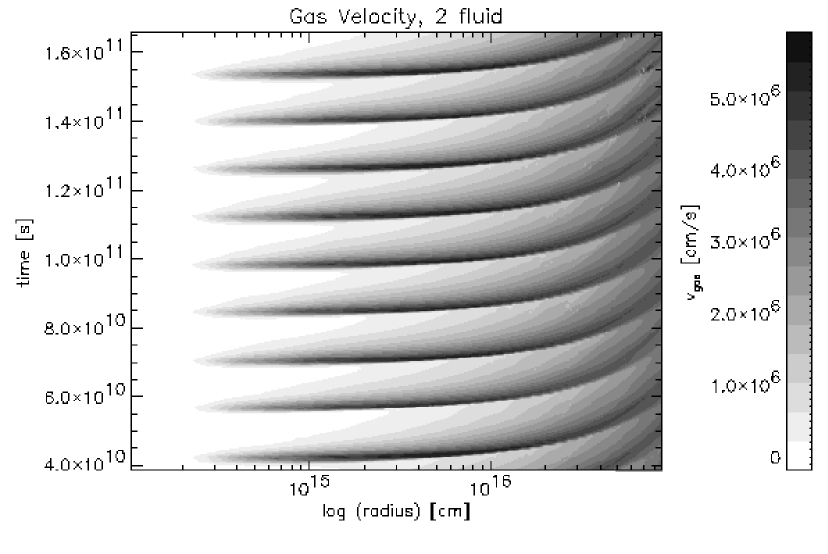
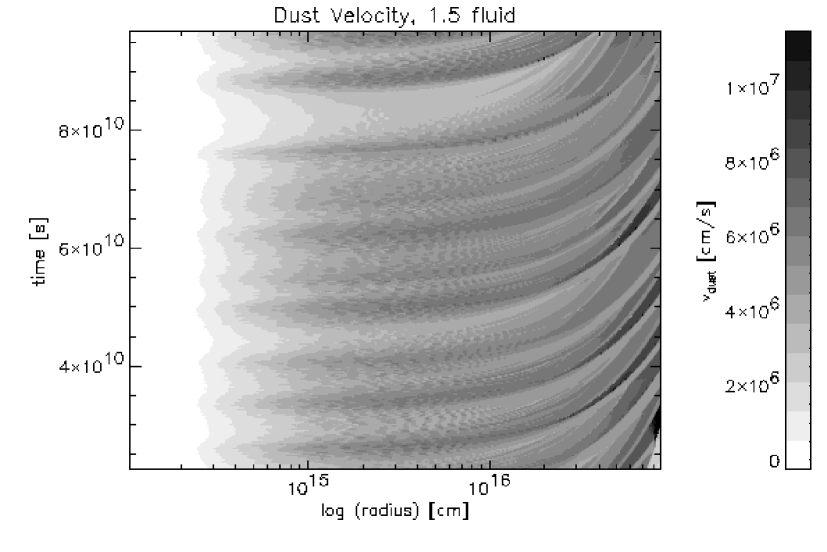
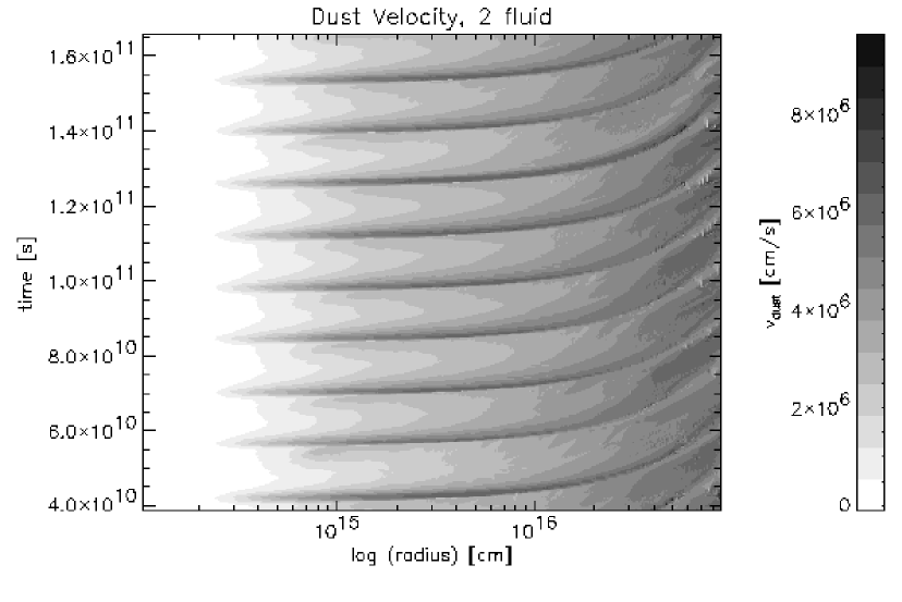
Figure 3: Gas and dust velocities as a function of radius and time for the 1.5 and the two–fluid model.

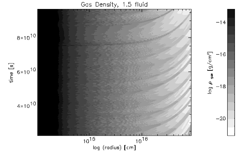
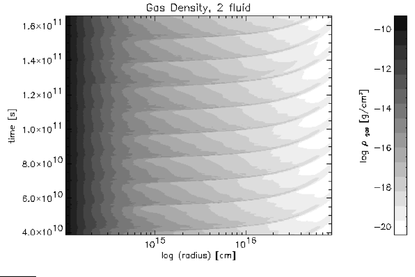
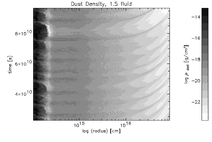
Figure 4: Gas and dust densities as a function of radius and time for the 1.5 and the two–fluid model.

Figs. 3 and 4 show, for the 1.5 and the two–fluid model, the gas and dust velocities and densities, as a function of radius and time. Throughout the whole grid, the fluctuations occurring in the two–fluid calculation are more regular that those in the 1.5–fluid model. The velocities of gas and dust in the momentum coupled calculation reach values that are up to 25% higher than in the two–fluid calculation. In the latter, matter is less accelerated than in the former, especially for radii larger than about $2\cdot 10^{16}$ cm. Probably, this is a result of non–equilibrium drift, which starts to appear around this radius (see Fig. 6). Non–equilibrium drift occurs when the time needed by a grain to reach its equilibrium drift velocity is long compared to the dynamical time scale. During a period of non–equilibrium drift, the gas is not being maximally accelerated and both gas and dust velocities will be lower than in a phase of equilibrium drift.
The gas density structure (Fig. 4) for the 1.5–fluid and the two–fluid calculation look similar. The main difference is that short time scale variations are present in the lower regions of the former, whereas large scale effects dominate the latter. The density structure plots for the dust show another difference: the perturbations in the 1.5–fluid flow appear as local increments of the density but in the two component flow the variations rather look like dips in the average profile. Maximum outflow density for gas and grains are in phase in the two–fluid model though, the “dust pulse” is significantly broader than but centered around the maximum in the gas outflow. This is not just the case in the upper parts of the envelope, where non–equilibrium drift is present, but also for smaller radii.

Figure 5: 1.5–fluid model. First column: gas and dust velocity (dashed line). The dot denotes the location of the critical point. Second column: gas and dust density (dashed line). Third column: drift velocity. Fourth column: average grain radius and grain nucleation rate (dashed line). The frames show (from top to bottom) the flow profile at 0, 30, 56, 81, 105, 132, 164, 197, 225, 252, 280, 310, 352 and 404 years after the first frame.

Figure 6: Two–fluid model. First column: gas and dust velocity (dashed line). The dot denotes the location of the critical point. Second column: gas and dust density (dashed line). Third column: drift velocity (dashed line) and equilibrium drift velocity (full line). Fourth column: average grain radius and grain nucleation rate (dashed line). The frames show (from top to bottom) the flow profile at 0, 32, 63, 93, 116, 131, 144, 156, 170, 189, 214, 245, 284 and 330 years after the first frame.

In Figs. 5 and 6 we plot a series of snapshots, displaying the evolution of various flow variables during one instability cycle for the 1.5 and the two–fluid model. For the 1.5–fluid calculation the drift velocity is, by definition, always equal to its equilibrium value, which shows a time dependent behavior. In the two–fluid flow we find that the drift velocity, out to approximately $10^{16}$ cm, equals the equilibrium value. At larger radii, small deviations from equilibrium drift are detected.
We want to stress that the fact that we see equilibrium drift in the lower and intermediate regions of the two component model only implies that equilibrium drift is established on a time scale shorter than the dynamical time scale. It does not however exclude the possibility that non–equilibrium drift occurs on shorter time scales, see Appendix A.

4.5 The origin of the mass loss variability

To investigate what causes the variability we will step through the frames of Fig. 6 for the two–fluid calculation. Thereafter, we will discuss the differences with the 1.5 fluid model. The mass loss rate of a stellar wind is determined in the subsonic region (see e.g. Lamers & Cassinelli (1999)), therefore in the following, when investigating the mechanism underlying the variability, we focus on this region, unless explicitly mentioned.
In Fig. 6, first frame, we see that the onset of the mass loss variability is the situation in which the dust has a velocity that is significantly higher than the gas velocity. This means that the residence time of a grain in the parts of the envelope where grains can grow is relatively short so that the average grain size will be on the small side. The smaller the grain, the more efficient radiation pressure will be, since small grains have a large surface to mass ratio and since we have assumed that the grain extinction cross section equals the geometrical cross section. Hence, radiative acceleration of grains is efficient and the velocity of the small grains increases further. Because position coupling is not imposed, the gas velocity can stay low and the drift velocity increases. Meanwhile (frames 2 and 3), the average grain radius decreases, grain acceleration becomes more efficient, the dust velocity grows, grains become smaller, and so forth. Also, the total mass density of the dust component in the innermost region decreases. When the grain radius in the subsonic region drops below a certain critical value, momentum transfer from grains to gas becomes efficient and the gas is accelerated (frame 4). This results in an increase of the gas density and hence of the number density of condensible particles. Since the grain nucleation rate is extremely sensitive to the molecular abundances, this results in an immediate increment of the nucleation rate (frame 4). The new production of condensation kernels leads to a further decrease of the average grain radius and an increase of the total grain mass density. Due to the large abundance of small grains, radiative acceleration and the transfer of momentum from grains to gas are very efficient, so that both gas and grains move out with high velocities (frames 5–8). On their way out, the small grains concentrate in a narrowing shell, since the decrease of the average grain radius in time coincides with an increase of their velocity. The gas develops a shell at the same time, as a result of the forming shock. The normal, Parker–type, stellar wind profile is now visible. We will refer to this phase as the “fast phase” (frame 5–9). Though not very clear from the figure, at the same time, a rarefaction wave moves in the opposite direction, leading to a decrease of the gas density, and of the number densities of the condensible species, below the sonic point. Although the density decrease is not so big, the nucleation rate reacts instantaneously (frames 9–13), showing a strong decrease traveling from the sonic point inwards. Hence, the passing of the rarefaction wave is immediately visible in the increase of the average grain radius because the production rate of new small grains decreases (frames 9–13). This illustrates the enormous sensitivity of the nucleation rate on the densities. The gradual increase, in time, of the average grain radius, brings about a less efficient radiative acceleration of the dust, hence a decrease of the grain velocity and a further increase of the grain radius, and so forth. This we will call the “slow phase” of the variability cycle (frames 10–14 and 1–4). Due to the larger grain size, the momentum transfer between grains and gas becomes less efficient, resulting in larger drift and dust velocities (frame 14). This brings us back to the situation in the first frame.
Crucial in the process of shell formation as described above are the two “turn–around” points, at which the nucleation rate starts to increase and decrease. First, at the end of the fast phase, the passage of the rarefaction wave triggers the end of a period of high nucleation rate. In the slow phase the gas–grain coupling has becomes less efficient, due to the larger average grain size. Grains then reach a higher drift velocity, become smaller and will again transfer their momentum efficiently to the gas, so that the latter can accelerate, increasing the density. This gives rise to favourable circumstances for grain nucleation again. Clearly, the behavior of the system during the slow phase is dominated by the existence of grain drift. This immediately explains why variability in the mass loss rate in a single fluid system is less well regulated (see Fig. 2).
When comparing Fig. 6 and Fig. 5, the absence of the slow phase in the variability cycle in the latter strikes the eye. This can be attributed to the imposed equilibrium drift in the 1.5–fluid flow. In the two–fluid system the drift velocity is directly influenced by the dynamics. In the 1.5–fluid model, however, the (equilibrium) drift velocity is only indirectly determined by the dynamics, namely via the (number) densities and the grain size. The fact that the variability character is still observed in this calculation is a consequence of the fact that the drift velocity, although not actively, does change as a function of time, in combination with the extreme sensitivity of the nucleation rate to the density and of the dynamics, via the drag force, on the grain size, and density. The sensitivity of the system is well visible in Fig. 5: any variation of the densities, grain size and nucleation rate is hardly visible (also because they are plotted logarithmically, ranging over many orders of magnitude) but the resulting variations in the velocity field are clearly present.

4.6 Comparison with observations

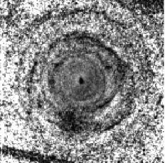
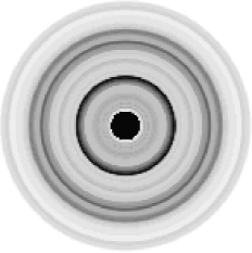
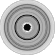
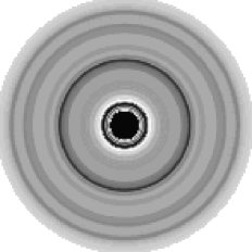
Figure 7: Upper left frame: Composite $B+V$ image of IRC +10216, with an average radial profile subtracted to enhance the contrast (adapted from Mauron & Huggins (1999)). Note that a few patches in the image are residuals of the removal of the brightest background objects, and these should be ignored. Other frames: series of snapshots of our 1.5–fluid calculation. Plotted is the dust column density, also with an average radial profile subtracted. The average radial profiles are calculated for each snaphot separately, hence the slight difference in color from plot to plot. The theoretical profiles are shown for ages 44, 118 and 211 years with respect to the first frame in Fig. 5. The size of our computational grid corresponds with the field of view of the observational image ($131\arcsec\times 131\arcsec$) and a distance of 120 pc.

To enable a qualitative comparison of our results with recent observations of IRC +10216 (Mauron & Huggins 1999; 2000), we have produced Fig. 7. The left frame is adapted from Mauron & Huggins (1999) (their Fig. 3). It shows the composite $B+V$ image of IRC +10216, with an average radial profile subtracted to enhance the contrast. We compare this image with the dust column density as a function of radius for a number of snapshots in our calculation. The size of our computational grid (extended to 1287 $R_{*}$) corresponds with the field of view of the observational image (131” $\times$ 131”) and a distance of 120 pc. We too, have subtracted an average radial density profile to enhance the contrast. Comparing dust column density to the observed intensity makes sense, since in the optically thin limit, the observed intensity, due to illumination by the interstellar radiation field is proportional to the column density along any line of sight (Mauron & Huggins (2000)). We used the results of the 1.5–fluid computation to produce Fig. 7 because there the short time scale structures are visible, whereas they are suppressed in the two–fluid model because the latter isn’t always second order accurate. Note that the fact that in our calculated images all shells appear to be perfectly round is simply due to our assumption of spherical symmetry. The two dimensional plots were produced by simply rotating the spherical symmetric profile. In view of the fact that our calculations indicate that the chemical–dynamic system that regulates the behavior of the envelope is extremely stiff and reacts violently to all kinds of changes, we think that it is rather unlikely that the observed circumstellar shells are indeed complete. It is intriguing to see that this idea is supported by the recent observations by Mauron & Huggins (2000), which show that most shells, although they may extend over much larger angles at lower levels, are prominent over about $45\degr$.
As was mentioned before, Fig. 7 only offers a qualitative comparison with the observations. It can, however be used to establish that the spacing of the shells, small scale structure inside, large scale structure outside, is similar in the observations and calculations. This, is not surprising however, since merging of shells of various widths is due to dispersion, as was mentioned in Section 4.4.

4.7 The timescale of mass loss variations

The characteristic time scale of the variability corresponds to the time needed by the rarefaction wave to cross the region between the sonic point and the innermost point of the nucleation zone. The width of this region is, depending on the phase, a few times $10^{14}$ to $10^{15}$ cm. The velocity of the rarefaction wave equals the gas velocity minus the local sound velocity and is typically a few times $10^{4}$ to $10^{5}$ cm s^-1, also depending on the phase of the variability. The resulting time scale is roughly 50 to 500 years, which indeed corresponds to the time separation between two maxima in the mass loss rate in our calculation.

4.8 Discussion

We found that the fact that the average grain size reacts strongly to the density structure is an essential ingredient for the formation of variability in the outflow. This explains why Mastrodemos et al. (1996) and Steffen & Schönberner (2000), who also performed time dependent, two–fluid computations, but did not take into account self consistent grain growth, did not encounter mass loss variations in the outflow.
Also, grain drift occurs to be essential for variations in the mass loss rate. If grains can drift with respect to the gas, they can form regions of higher (or lower) density and/or size independently from the gas.
Periodic variability in the mass loss rate occurs in both the 1.5–fluid and the two–fluid calculations, because grains are allowed to drift in both cases. Both calculations give somewhat different results, though. Probably, assuming equilibrium drift a priori, as was done in the 1.5–fluid computation, influences the results, even if the grains in the two–fluid model turn out to drift at the equilibrium drift velocity as well. There are two reasons for this. First, the fact that equilibrium drift has established itself at the end of a numerical time step, does not mean that there has been equilibrium always during this specific time step. Hence, integration of the drag force over the time step provides a better value of the momentum transfer than multiplication of the drag force with the duration of the time step, c.f. Appendix A. Second, the value of the equilibrium drift velocity in the 1.5–fluid calculation is indirectly determined by the dynamics, whereas in the two–fluid case there is a direct influence. Also, the fact that the 1.5-fluid calculation is second order accurate, but in the two-fluid calculation this level of accuracy is not always achieved, will lead to differences in the results.
We have not taken into account radiative transfer to solve the energy structure in the envelope. Also, we used a grey absorption coefficient in the radiative force and we did not calculate the grain temperature. These are severe limitations of the model. However, we believe that they do not influence the general conclusion that dynamics and chemistry together can lead to time dependent structures. It is more likely that taking into account the temperature structure determined by the optical properties of the grain population will make the variability even more pronounced. This is inferred from previous calculations by Fleischer et al. (1992) in which the interaction between atmospheric dynamics and radiative transfer was solved, imposing a time dependent inner boundary. Recently, Winters et al. (2000) performed similar calculations, also without the piston at the inner boundary. Their results also indicate that the coupling between the sensitive grain chemistry and the dynamics can lead to variability in the wind.
The role of the inner boundary in calculations as presented here is extremely important. It is possible to generate wind variability using a time dependent inner boundary. We did not do this: the inner boundary that we have used was created to have as little influence on the results as possible. It consists of a fixed advective flux which can be modified by a diffusion term. The diffusive contribution to the flux is proportional to the gradients of the flow variables near the inner boundary, i.e. it is not externally prescribed. This is a realistic approach, since the inner boundary is located in the subsonic regime, where communication with lower layers is still possible. In this respect a completely fixed inner boundary would be less realistic.
We have referred to the quasi–periodic structure in our models as “shells”. In order to prove that the structure is truly created in the form of spherical shells one should perform three dimensional hydrodynamics. Higher dimensionality will be a topic of future research. Shell structure is observed around only a small number of Post–AGB objects and PNe. It is possible that the majority of objects doesn’t have shells. A stationary wind can definitely exist if for some reason the equilibrium drift velocity is relatively low. This can be the case if the luminosity of the star is low. This will limit the mutual motion of both fluids and hence the value of the gas to dust density ratio so that the outflow will remain more smooth.

5 Conclusion

Our calculations suggest that the sensitive interplay of grain nucleation and dynamics, in particular grain drift, leads to quasi–periodic winds on the AGB. The characteristic time scale for the variability corresponds to the crossing of the subsonic nucleation zone by the rarefaction wave. This time scale also matches recent observations of IRC +10216.
More generally, we would like to stress that two–fluid hydrodynamics is important in order to reach self–consistency of the modeling method since the validity of the assumption of equilibrium drift is hard to check. If equilibrium drift is applied, it should be calculated by demanding the grains and the gas to be equally accelerated, rather than by equating the drag force and the radiation pressure on grains, because grains do have mass.
Observations also imply that gas and grains may not be spatially coupled (Sylvester et al. (1999)) and that variations in the gas to dust ratio in the outflow may arise (Omont et al. (1999)).

Appendix A Calculating the drag force

To derive an expression for the drag force, we need to know about the time evolution of the drift velocity. The gas–grain system will always evolve towards a state in which grains drift at the equilibrium drift speed, hence in which gas and grains undergo the same acceleration. If, or how rapidly this state is reached depends on the time needed to establish the equilibrium relative to the dynamical time scale. If one assumes that equilibrium drift is always valid, the momentum transfer in a numerical time step can simply be calculated by using the equilibrium value of the drift velocity in Eq.(8) and multiplying the drag force by the duration of the time step. However, if, during a fraction of the numerical time step, the drift velocity is lower than the equilibrium value, assuming equilibrium drift when calculating the drag force will overestimate the momentum transfer. This is illustrated in Fig. 8. Although the error for a single time step may be very small, the implications may be large for the time dependent calculation. Note that, when assuming equilibrium drift, one fixes the value of the drift velocity so that the gas and the dust velocities are no longer independent flow variables. Therefore, when calculating the momentum transfer assuming equilibrium drift one is forced to do a 1.5-fluid calculation rather than a full two-fluid calculation.

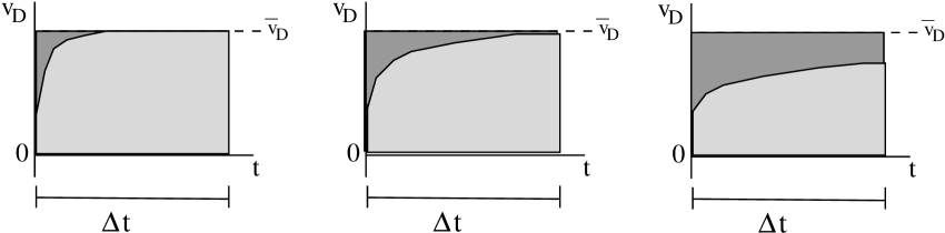
Figure 8: Evolution towards equilibrium drift within a single time step: because it may take some time to establish equilibrium, calculating the momentum transfer by simply multiplying the drag force (which is proportional to $v_{\mathrm{D}}^{2}$) with $\Delta t$ overestimates the momentum transfer. The difference between the exact calculation and the equilibrium calculation increases with the time required to establish equilibrium drift and is represented by the dark color in the figures.

We will, hereafter, derive an expression for the time evolution of the drift velocity. With this expression we can calculate the momentum transfer as the integral of the drag force over the numerical time step. No assumptions about the final drift velocity need to be made and the derived expression can be used in a full two-fluid calculation.
It is important to note that even if we find equilibrium drift in the two component calculation this does not imply that it would have been justified to assume equilibrium drift a priori. This can be seen from Fig. 8. In both the first and the second panel equilibrium drift is established within the duration of the numerical time step, $\Delta t$, i.e., in both cases the output of the hydrodynamics indicates equilibrium drift. Assuming equilibrium drift throughout the time step would however only slightly overestimate the momentum transfer in the first panel whereas is the second panel the difference between the exact integral of the drag force over the time step and equilibrium approximation would be much bigger.

A.1 An analytical expression for the momentum transfer rate

In this section we will derive an expression for the time evolution of the drift velocity. Using this expression we can calculate the rate at which momentum is transfered from grains to gas.
Fig. 9 shows the six possible cases for reaching equilibrium drift. Note that both the initial drift and the equilibrium value can be negative if the grains are less accelerated than the gas.

Figure 9: Evolution towards equilibrium drift for various initial drift velocities. Upper panels: $g_{\mathrm{D,tot}}>0\rightarrow\bar{v}_{\mathrm{D}}>0$, lower panels: $g_{\mathrm{D,tot}}<0\rightarrow\bar{v}_{\mathrm{D}}<0$

We assume that the gas–grain interactions are completely inelastic. Furthermore, we assume that after a collision with a grain, a gas particle shares the acquired momentum with the surrounding gas instantaneously (thermalization). This is realistic, since the mean free path of gas–gas collisions is very small compared to the mean free path for gas–grain encounters. We will not take into account thermal motion because this enables us to derive an analytic expression for the drag force. This will result in a somewhat lower momentum transfer in the subsonic region. Farther out, the drift velocity of the grains will dominate the collision rate anyway.
First, consider the motion of an individual gas particle between two subsequent collisions with a grain:

$$v_{\mathrm{g}}\rightarrow v_{\mathrm{g}}+g_{\mathrm{g,tot}}\delta t+\frac{n_{\mathrm{d}}}{n_{\mathrm{g}}}\frac{\Delta p}{m_{\mathrm{g}}}$$ (11)

Here, $v_{\mathrm{g}}$ is the velocity of the particle, after the previous collision, $g_{\mathrm{g,tot}}$ is the total acceleration due to gravity and the pressure gradient (but not the drag force), $\delta t$ is the time interval between two collisions. The last term represents the increase in the velocity as a result of the encounter with the grain, and the (instantaneous) redistribution of the momentum amongst the gas. $\Delta p$ is the amount of momentum transferred in a single gas–grain collision,

$$\Delta p=\frac{m_{\mathrm{g}}m_{\mathrm{d}}}{m_{\mathrm{g}}+m_{\mathrm{d}}}u_{\mathrm{D}}$$ (12)

where $u_{\mathrm{D}}$ is the velocity of a grain with respect to the gas immediately before the collision, $m_{\mathrm{g,d}}$ are the masses of a gas particle (i.e. the mean molecular weight) and the (average) grain mass. A similar equation for the dust grain is

$$v_{\mathrm{d}}\rightarrow v_{\mathrm{d}}+g_{\mathrm{d,tot}}\delta t-\frac{\Delta p}{m_{\mathrm{d}}}$$ (13)

The drift velocity after a collision, $v_{\mathrm{D}}$, can now be expressed in terms of the drift velocity immediately before the encounter, $u_{\mathrm{D}}$, as follows:

$$v_{\mathrm{D}}=\Omega u_{\mathrm{D}}$$ (14)

in which

$$\Omega=\frac{\rho_{\mathrm{g}}m_{\mathrm{d}}-\rho_{\mathrm{d}}m_{\mathrm{g}}}{\rho_{\mathrm{g}}(m_{\mathrm{g}}+m_{\mathrm{d}})}$$ (15)

$$u_{\mathrm{D}}=u_{\mathrm{d}}-u_{\mathrm{g}}=v_{\mathrm{d}}-v_{\mathrm{g}}+(g_{\mathrm{d,tot}}-g_{\mathrm{g,tot}})\delta t$$ (16)

In the following, we will write $g_{\mathrm{D,tot}}$ for the relative acceleration, $g_{\mathrm{d,tot}}-g_{\mathrm{g,tot}}$. The “mean free travel time”, $\delta t$, of a grain can be found by solving the quadratic equation for the mean free path, $\lambda$, of a grain

$$\lambda=v_{\mathrm{D}}\delta t+\frac{1}{2}g_{\mathrm{D,tot}}\delta t^{2}$$ (17)

Note that the mean free path can become negative if the initial drift velocity, $v_{\mathrm{D}}$, and/or the relative acceleration $g_{\mathrm{D,tot}}$ is negative. If grains are not significantly accelerated between two subsequent collisions with gas particles, i.e. if $v_{\mathrm{D}}\gg g_{\mathrm{D,tot}}\delta t$, Eq.(17) simply becomes

$$\lambda=v_{\mathrm{D}}\delta t$$ (18)

so that $\delta t=\lambda/v_{\mathrm{D}}$. On the other hand, if the acceleration of a grain between two collisions is so large that its initial (drift) velocity is negligible, Eq.(17) reads

$$\lambda=\frac{1}{2}g_{\mathrm{D,tot}}\delta t^{2}$$ (19)

and $\delta t=\sqrt{2\lambda/g_{\mathrm{D,tot}}}$. The boundary between the two regimes lies at the drift velocity for which $2v_{\mathrm{D}}=g_{\mathrm{D,tot}}\delta t$. With $\delta t$ given by the solution of Eq.(17) we find that if

$$|v_{\mathrm{D}}|<\frac{1}{2}\sqrt{\lambda g_{\mathrm{D,tot}}}$$ (20)

Eq.(19) can be used instead of Eq.(17). In the current context of dust forming stellar winds, the quantity $\Omega$ will always be nearly equal to unity, so that $\bar{v}_{\mathrm{D}}\gg\frac{1}{2}\sqrt{\lambda g_{\mathrm{D,tot}}}$. Hence, the zone in velocity space where grain acceleration is significant is extremely narrow. If the drift velocity is zero at some time (see e.g. Fig. 9.c,f), it follows from Eq.(14), (16) and (19) that the drift velocity will be larger than $\frac{1}{2}\sqrt{\lambda g_{\mathrm{D,tot}}}$ after a single collision unless $\Omega<1/\sqrt{8}$. This implies that we can safely apply Eq.(18) for all values of $v_{\mathrm{D}}$.
In the following we will present a method to derive an expression for the momentum transfer, which applies to all possible scenarios (see Fig. 9) to reach equilibrium drift. We limit ourselves to the derivation for the case $g_{\mathrm{D,tot}}>0$ (Fig. 9.a,b,c), the derivation for negative acceleration is analogous.
Application of Eq.(18) and Eq.(16) in Eq.(14) gives rise directly to a recurrence relation for $v_{\mathrm{D}}$:

$$v_{\mathrm{D}}(t_{i+1})=\Omega u_{\mathrm{D}}(t_{i+1})=\Omega\left(v_{\mathrm{D}}(t_{i})+\frac{g_{\mathrm{D,tot}}\lambda}{v_{\mathrm{D}}(t_{i})}\right)$$ (21)

From this, and $\delta t$ given by Eq.(18), a differential equation for the drift velocity as a function of time can be derived:

$$\frac{\Delta v_{\mathrm{D}}}{\Delta t}\simeq\frac{\mathrm{d}v_{\mathrm{D}}}{\mathrm{d}t}=\frac{\Omega-1}{\lambda}v_{\mathrm{D}}^{2}+\Omega g_{\mathrm{D,tot}}$$ (22)

This equation can be easily solved for $t(v_{\mathrm{D}})$,

$$t(v_{\mathrm{D}}) = \frac{\lambda}{\sqrt{\Omega(\Omega-1)g\lambda}}$$ (23)

$$\Biggl{[} \arctan\left(\frac{(\Omega-1)v_{\mathrm{D}}(t)}{\sqrt{\Omega(\Omega-1)g\lambda}}\right)\Biggr{.}-$$

. $$\arctan\left(\frac{(\Omega-1)v_{\mathrm{D}}(0)}{\sqrt{\Omega(\Omega-1)g\lambda}}\right)\,\Biggr{]}$$

where $g$ stands for $g_{\mathrm{D,tot}}$.
First, consider the case where $v_{\mathrm{D}}(0)>0$ (and $g>0$). In this case the mean free path $\lambda$ will always be positive. Because $\Omega$ is always smaller than unity and $\lambda$ and $g$ have equal signs this is rewritten as

$$t(v_{\mathrm{D}}) = \frac{\lambda}{\sqrt{\Omega(1-\Omega)g\lambda}}$$ (24)

$$\Biggl{[} \mbox{arctanh}\left(\frac{(1-\Omega)v_{\mathrm{D}}(t)}{\sqrt{\Omega(1-\Omega)g\lambda}}\right)-\Biggr{.}$$

. $$\mbox{arctanh}\left(\frac{(1-\Omega)v_{\mathrm{D}}(0)}{\sqrt{\Omega(1-\Omega)g\lambda}}\right)\,\Biggr{]}$$

This expression can be simplified by realizing that from Eq.(21) it follows that the equilibrium drift velocity is given by

$$\bar{v}_{\mathrm{D}}=\sqrt{\frac{\Omega}{1-\Omega}\lambda g}$$ (25)

and that the equilibration time scale is

$$\tau_{\mathrm{eq}}=\frac{1}{\sqrt{\Omega(1-\Omega)g/\lambda}}$$ (26)

so that

$$t(v_{\mathrm{D}})=\tau_{\mathrm{eq}} \left[\mbox{arctanh}\left(\frac{v_{\mathrm{D}}(t)}{\bar{v}_{\mathrm{D}}}\right)-\right.$$ (27)

$$\left.\,\,\,\mbox{arctanh}\left(\frac{v_{\mathrm{D}}(0)}{\bar{v}_{\mathrm{D}}}\right)\right]$$

$$=\tau_{\mathrm{eq}}\ \,\,\,\mbox{arctanh}\left(\frac{(v_{\mathrm{D}}(t)-v_{\mathrm{D}}(0))\bar{v}_{\mathrm{D}}}{\bar{v}_{\mathrm{D}}^{2}-v_{\mathrm{D}}(t)v_{\mathrm{D}}(0)}\right)$$ (28)

Note that addition of the arctanh terms causes the expression to be valid for initial values $v_{\mathrm{D}}(0)>\bar{v}_{\mathrm{D}}$ (see Fig. 9.b) as well. Inversion leads to an expression for the drift velocity as a function of time:

$$v_{\mathrm{D}}(t)=\bar{v}_{\mathrm{D}}\frac{v_{\mathrm{D}}(0)+\bar{v}_{\mathrm{D}}\Theta(t)}{\bar{v}_{\mathrm{D}}+v_{\mathrm{D}}(0)\Theta(t)}$$ (29)

with

$$\Theta(t)=\mbox{tanh}(t/\tau_{\mathrm{eq}})$$ (30)

The drag force (density) is the product of the number of gas–grain collisions per unit volume and time and the momentum transfer per collision. In Eq.(8), the amount of momentum transfer in a single collision was simply assumed to be $m_{\mathrm{g}}v_{\mathrm{D}}$, now we use the more accurate form for $\Delta p$ which follows from Eqs.(12), (14), (18). With $\lambda=1/\Sigma_{\mathrm{d}}n_{\mathrm{g}}$ we then find

$$f_{\mathrm{drag}}=\Sigma_{\mathrm{d}}\rho_{\mathrm{g}}\frac{n_{\mathrm{g}}n_{\mathrm{d}}}{n_{\mathrm{g}}-n_{\mathrm{d}}}|v_{\mathrm{D}}|v_{\mathrm{D}}$$ (31)

The standard way to calculate the amount of momentum transfer per numerical time step is simply multiplying the drag force with the duration of the time step. Now that we have derived an expression for the drift velocity as a function of time we can calculate the momentum transfer more accurate, by integrating Eq.(31), assuming $n_{\mathrm{g,d}},m_{\mathrm{g,d}}$ are constant:

$$\int_{0}^{\tau}f_{\mathrm{drag}}\mbox{d}t=\Sigma_{\mathrm{d}}\rho_{\mathrm{g}}\frac{n_{\mathrm{g}}n_{\mathrm{d}}}{n_{\mathrm{g}}-n_{\mathrm{d}}}\tau_{\mathrm{eq}}\bar{v}_{\mathrm{D}}^{2}\Biggl{[}\frac{\tau}{\tau_{\mathrm{eq}}}+$$

$$\left(\frac{v_{\mathrm{D}}(0)}{\bar{v}_{\mathrm{D}}}-\frac{\bar{v}_{\mathrm{D}}}{v_{\mathrm{D}}(0)}\right)\left(\frac{v_{\mathrm{D}}(0)\tanh(\tau/\tau_{\mathrm{eq}})}{v_{\mathrm{D}}(0)\tanh(\tau/\tau_{\mathrm{eq}})+\bar{v}_{\mathrm{D}}}\right)\Biggr{]}$$ (32)

If the initial drift velocity and the total acceleration have opposite sign ($v_{\mathrm{D}}(0)<0,g>0$, see Fig. 9.c) the integral representing the total momentum transfer is split into two parts,

$$\int_{0}^{\tau}f_{\mathrm{drag}}\mbox{d}t=\int_{0}^{t(v_{D}=0)}f_{\mathrm{drag}}\mbox{d}t+\int_{t(v_{D}=0)}^{\tau}f_{\mathrm{drag}}\mbox{d}t$$ (33)

where $t(v_{\mathrm{D}}=0)$ follows from Eq.(23):

$$t(v_{\mathrm{D}}=0) = \frac{-\lambda}{\sqrt{\Omega(\Omega-1)g\lambda}}$$ (34)

$$\arctan\left(\frac{(\Omega-1)v_{\mathrm{D}}(0)}{\sqrt{\Omega(\Omega-1)g\lambda}}\right)$$

Note that the mean free path of a grain, $\lambda$, is negative as long as the drift velocity is negative. The second term in Eq.(33) is calculated as in the case $v_{\mathrm{D}}(0)>0$, simply taking $v_{\mathrm{D}}(0)=0$. In order to compute the first term, Eq.(23) is inverted. We find

$$v_{\mathrm{D}}(t)=\bar{v}_{\mathrm{D}}\frac{v_{\mathrm{D}}(0)+\bar{v}_{\mathrm{D}}\Theta^{\prime}(t)}{\bar{v}_{\mathrm{D}}-v_{\mathrm{D}}(0)\Theta^{\prime}(t)}$$ (35)

in which

$$\Theta^{\prime}(t)=\mbox{tan}(t/\tau^{\prime}_{\mathrm{eq}})$$ (36)

$$\bar{v}_{\mathrm{D}}=\sqrt{\frac{\Omega}{\Omega-1}\lambda g}$$ (37)

$$\tau^{\prime}_{\mathrm{eq}}=\frac{1}{\sqrt{\Omega(\Omega-1)g/\lambda}}$$ (38)

Inserting this into Eq.(31) and integrating over the interval $t=0,t(v_{D}=0)$, we obtain

$$\int_{0}^{t(v_{D}=0)}f_{\mathrm{drag}}\mbox{d}t = -\Sigma_{\mathrm{d}}\rho_{\mathrm{g}}\frac{n_{\mathrm{g}}n_{\mathrm{d}}}{n_{\mathrm{g}}-n_{\mathrm{d}}}\tau^{\prime}_{\mathrm{eq}}\bar{v}_{\mathrm{D}}^{2}$$ (39)

$$\left[-\frac{v_{\mathrm{D}}(0)}{\bar{v}_{\mathrm{D}}}+\arctan\left(\frac{v_{\mathrm{D}}(0)}{\bar{v}_{\mathrm{D}}}\right)\right]$$

Note that the minus sign accounts for the fact that the momentum transfer contains an integral over $|v_{\mathrm{D}}|v_{\mathrm{D}}$ rather than an integral over $v_{\mathrm{D}}^{2}$. Finally, for the complete integral, Eq.(33), we find

$$\int_{0}^{\tau}f_{\mathrm{drag}}\mbox{d}t=\Sigma_{\mathrm{d}}\rho_{\mathrm{g}}\frac{n_{\mathrm{g}}n_{\mathrm{d}}}{n_{\mathrm{g}}-n_{\mathrm{d}}}\tau_{\mathrm{eq}}\bar{v}_{\mathrm{D}}^{2}$$

$$\left[\frac{\tau}{\tau_{\mathrm{eq}}}-\mbox{tanh}\left(\frac{\tau}{\tau_{\mathrm{eq}}}+\mbox{arctan}\left(\frac{v_{\mathrm{D}}(0)}{\bar{v}_{\mathrm{D}}}\right)\right)+\frac{v_{\mathrm{D}}(0)}{\bar{v}_{\mathrm{D}}}\right]$$ (40)

As was to be expected Eq.(32) and Eq.(40) are equal if $v_{\mathrm{D}}(0)=0$.
Similar expressions for the total momentum transfer can be calculated in the case of negative total acceleration (see Fig. 9.d,e,f).
The above formulations for the momentum transfer, in which no assumptions about the value of the drift velocity or the completeness of momentum coupling have been made, can be used as source terms in the momentum equations.

A.2 Calculation of the equilibrium drift velocity

We have used the terms equilibrium drift velocity and limiting velocity as equivalent. Here, we will show that both are indeed the same. We equate the acceleration of the gas and the dust, rather than equating the drag force and the radiation pressure of grains. In the latter case one implicitly assumes that grains do not have mass whereas the former leads to a general expression for the equilibrium drift velocity.
From the equation of motion of a gas element,

$$\frac{\mathrm{d}v_{\mathrm{g}}}{\mathrm{d}t}=g_{\mathrm{g,tot}}+\frac{f_{\mathrm{drag}}}{\rho_{\mathrm{g}}}$$ (41)

and its counterpart for a grain,

$$\frac{\mathrm{d}v_{\mathrm{d}}}{\mathrm{d}t}=g_{\mathrm{d,tot}}-\frac{f_{\mathrm{drag}}}{\rho_{\mathrm{d}}}$$ (42)

we find that grains and gas are equally accelerated, and hence the drift velocity has reached its equilibrium value, if

$$g_{\mathrm{D,tot}}=\frac{\rho_{\mathrm{d}}+\rho_{\mathrm{g}}}{\rho_{\mathrm{d}}\rho_{\mathrm{g}}}f_{\mathrm{drag}}$$ (43)

With Eq.(31), the equilibrium drift velocity is

$$\bar{v}_{\mathrm{D}}=\sqrt{\frac{m_{\mathrm{d}}(n_{\mathrm{g}}-n_{\mathrm{d}})}{\rho_{\mathrm{d}}+\rho_{\mathrm{g}}}g_{\mathrm{D,tot}}\lambda}$$ (44)

Thus, we have now derived an expression for the equilibrium drift velocity without having to assume complete momentum coupling. This expression is indeed the same as Eq.(25), which represents the limiting drift velocity.

References

- Berruyer (1991) Berruyer, N., 1991, A&A 249, 181
- Berruyer & Frisch (1983) Berruyer, N., & Frisch, H., 1983, A&A 126, 269
- Boris (1976) Boris, J., 1976, NRL Mem. Rep. 3237
- Bowen (1988) Bowen, G., 1988, Ap.J. 329, 299
- Dominik (1992) Dominik, C., 1992, Ph.D. thesis, Technischen Universität Berlin
- Dorfi & Höfner (1991) Dorfi, E., & Höfner, S., 1991, A&A 248, 105
- Fleischer et al. (1992) Fleischer, A., Gauger, A., & Sedlmayr, E., 1992, A&A 266, 321
- Fleischer et al. (1995) Fleischer, A., Gauger, A., & Sedlmayr, E., 1995, A&A 297, 543
- Gail et al. (1984) Gail, H.-P., Keller, R., & Sedlmayr, E., 1984, A&A 133, 320
- Gail & Sedlmayr (1987) Gail, H.-P., & Sedlmayr, E., 1987, A&A 171, 197
- Gail & Sedlmayr (1988) Gail, H.-P., & Sedlmayr, E., 1988, A&A 206, 153
- Gail & Sedlmayr (1999) Gail, H.-P., & Sedlmayr, E., 1999, A&A 347, 594
- Gilman (1972) Gilman, R. C., 1972, ApJ 178, 423
- Harrington & Borkowski (1994) Harrington, J. P., & Borkowski, K. J., 1994, BAAS 26, 1469
- Höfner et al. (1995) Höfner, S., Feuchtinger, M., & Dorfi, E., 1995, A&A 297, 815
- Icke (1991) Icke, V., 1991, A&A 251, 369
- Krüger et al. (1994) Krüger, D., Gauger, A., & Sedlmayr, E., 1994, A&A 290, 573
- Krüger & Sedlmayr (1997) Krüger, D., & Sedlmayr, E., 1997, A&A 321, 557
- Lamers & Cassinelli (1999) Lamers, H., & Cassinelli, J., 1999, Introduction to stellar winds, Cambridge University Press
- MacGregor & Stencel (1992) MacGregor, K., & Stencel, R., 1992, ApJ 397, 644
- Mastrodemos et al. (1996) Mastrodemos, N., Morris, M., & Castor, J., 1996, ApJ 468, 851
- Mauron & Huggins (1999) Mauron, N., & Huggins, P. J., 1999, A&A 349, 203
- Mauron & Huggins (2000) Mauron, N., & Huggins, P. J., 2000, A&A 359, 707
- Ney et al. (1975) Ney, E. P., Merrill, K. M., Becklin, E. E., Neugebauer, G., & Wynn-Williams, C. G., 1975, ApJ 198, L129
- Omont et al. (1999) Omont, A., Ganesh, S., Alard, C., et al., 1999, A&A 348, 755
- Sahai et al. (1998) Sahai, R., Trauger, J. T., Watson, A. M., et al., 1998, ApJ 493, 301
- Schaaf (1963) Schaaf, S., 1963, in Handbuch der Physik, volume VIII/2, Springer Verlag, Berlin, Göttingen, Heidelberg, p. 591
- Sedlmayr (1997) Sedlmayr, E., 1997, in Stellar Atmospheres: Theory and Observations; EADN Astrophysics School IX, Brussels, Belgium, 10 – 19 September 1996 / J.P. de Greve et al. (ed.), p. 89
- Steffen & Schönberner (2000) Steffen, M., & Schönberner, D., 2000, A&A 357, 180
- Steffen et al. (1997) Steffen, M., Szczerba, R., Men’shchikov, A., & Schönberner, D., 1997, A&AS 126, 39
- Steffen et al. (1998) Steffen, M., Szczerba, R., & Schönberner, D., 1998, A&A 337, 149
- Sylvester et al. (1999) Sylvester, R. J., Kemper, F., Barlow, M. J., et al., 1999, A&A 352, 587
- Winters et al. (2000) Winters, J. M., Le Bertre, T., Jeong, K., Helling, C., & Sedlmayr, E., 2000, A&A 361, 641
- Winters et al. (1994) Winters, J. M., Dominik, C., & Sedlmayr, E., 1994, A&A 288, 255