The Optical/Infrared Astronomical Quality of High Atacama Sites. II. Infrared Characteristics

Abstract

We discuss properties of the atmospheric water vapor above the high Andean plateau region known as the Llano de Chajnantor, in the Atacama Desert of northern Chile. A combination of radiometric and radiosonde measurements indicate that the median column of precipitable water vapor (PWV) above the plateau at an elevation of 5000 m is approximately 1.2 mm. The exponential scaleheight of the water vapor density in the median Chajnantor atmosphere is 1.13 km; the median PWV is 0.5 mm above an elevation of 5750 m. Both of these numbers appear to be lower at night. Annual, diurnal and other dependences of PWV and its scaleheight are discussed, as well as the occurrence of temperature inversion layers below the elevation of peaks surrounding the plateau. We estimate the background for infrared observations and sensitivities for broad band and high resolution spectroscopy. The results suggest that exceptional atmospheric conditions are present in the region, yielding high infrared transparency and high sensitivity for future ground–based infrared telescopes.

Subject Headings: Astronomical instrumentation, methods and techniques: atmospheric effects, site testing.

1 Introduction

Atmospheric molecules are responsible for band absorption of cosmic radiation. In the near and mid–IR, the most important absorbers are the triatomic molecules H₂O, CO₂ and O₃. Between absorption bands, partially transparent windows appear, making astronomical observations possible in the near and mid–IR from the ground. The atmosphere is virtually opaque between 50 and 200 $\mu$m from all sites on the ground, making that wavelength region the exclusive territory of airborne and space observatories. Water vapor also dominates absorption in the far IR and submm region; atmospheric windows appear near 200, 350, 450, 600, 750 and 870 $\mu$m; in this spectral region transparency is significant only in dry, high altitude sites (Tokunaga 1998; Wolfe & Zissis 1978). H₂O molecules have a short residence time (a few days) in the atmosphere and their concentration is highly variable. Thus, the characterization of potential astronomical sites for operation in the IR and submm spectral regimes depends very strongly on measurements of atmospheric water vapor.

In a companion paper (Giovanelli et al. 2000; Paper I), we have discussed the desirability of ascertaining the quality of high altitude sites for astronomical research in the optical and infrared parts of the spectrum. Paper I describes briefly the Atacama desert region and, as part of a site survey campaign, the results of optical seeing measurements. Here, we review the results of measurements carried out in the Andean plateau known as the Llano de Chajnantor, in the Atacama desert of northern Chile, aimed at gauging the atmospheric transparency and emissivity in the infrared. The main characteristics of the atmospheric water vapor in the region are discussed: its absolute amount, annual, seasonal and diurnal variations, as well as its vertical distribution. The latter information provides indications of the relative infrared transparency at sites at varying elevation above the plateau, even of those currently inaccessible for deployment of testing equipment.

In Section 2  we briefly describe the data utilized for the analysis; in Section 3, statistics of the total precipitable water vapor (PWV, defined as the atmospheric column density of water vapor) are given, and in Section 4  the vertical distribution of PWV is analyzed, with estimates of its value expected for candidate sites for an optical/IR telescope. Finally, in Section 5  we estimate atmospheric transparency, emissivity and telescope sensitivities in the infrared, for a range of possible water vapor conditions.

2 Data Sources

We make use of two kinds of data in this report:

• Atmospheric opacities measured with automated tipping radiometers at 225 GHz and at 183 GHz. These instruments are operated by the National Radio Astronomy Observatory (NRAO) , the European Southern Observatory (ESO) and the Onsala Space Observatory. Data taken since April 1995 can be found at http://www.tuc.nrao.edu/mma/sites/Chajnantor and http://alma.sc.eso.org. We shall refer to summaries of relevant data products as given at those sites.

• Radiosonde data from balloon launches initiated in October 1998, jointly operated by Cornell University, NRAO, ESO and the Smithsonian Astrophysical Observatory. We will summarize results from radiosondes launched between October 1998 and August 2000. Details on individual launches can be found at http://www.astro.cornell.edu/atacama/sondedata.html and at the above web sites of NRAO (Radford 2000) and ESO (Otarola 2000). A more detailed analysis of the full radiosonde data set will be presented in a forthcoming paper, by the ‘radiosonde consortium’.

Tipping radiometers yield values of the atmospheric opacity, from which estimates of PWV above the radiometer location can be inferred. Radiosondes, on the other hand, provide vertical profiles of atmospheric parameters (temperature, pressure, relative humidity, wind speed and direction); from those, the water vapor density distribution and thus the PWV above any altitude can be inferred. Several summits, which are potentially attractive sites for infrared telescopes, have no access roads and thus installation and access to equipment at those locations is impractical. The free atmosphere parameters obtained from radiosonde launches provide a rough approximation of conditions that would be found at those summits. In the remainder of this paper, we shall always refer to PWV at zenith.

The sites for radiometer data taking and radiosonde launches are within one km from each other, near latitude S 23^∘ 01’, longitude W 67^∘ 46’, at an altitude near 5000 m above mean sea level. It should be kept in mind that, depending on wind speed and direction, a sonde flight samples an oblique path through the atmosphere, rather than a vertical one. In strong wind. a sonde profile typically spans tens of km in horizontal range. However, since most of the atmospheric water vapor is generally distributed within a few km from the ground, the effective sampling of most of the PWV corresponds to a horizontal range of only a few km from the launch site. Given the prevalent wind direction (see Paper I for details), sondes usually fly towards the East over unpopulated terrain, with ground elevation ranging between 4500 m and 5800 m above mean sea level.

In this paper, we shall use data from 108 radiosonde launches distributed as follows: 8, 10 and 16 launches in October, November and December 1998 respectively; 1, 5 and 33 in February, March and November 1999 respectively; 11, 18 and 6 in June, July and August 2000 respectively. Thirty were launched in nighttime hours (UT 01 to 11 hours), 65 in daytime (UT 12 to 21 hours) and 13 in the early evening (UT 22 to 00 hours). For each sonde profile we integrate the water vapor to obtain PWV above the plateau level of 5050 m, PWV above the elevation of 5400 m (equivalent to the summit of Cerro Honar) and PWV above 5750 m (equivalent to the summit of Cerro Chascón). We also compute the height above the plateau at which water vapor density drops to $1/e$ of the value at the plateau level, $h_{e}$, an indication of the exponential scaleheight of the water vapor layer. Since the water vapor distribution is most often not close to an exponential, we also measure ($h_{1/2}$), the height at which PWV drops to 50% of the value at the plateau level. Finally, we note the location of temperature inversions, which often are seen trapping large fractions of the total PWV below them. The derivation of these parameters and a detailed presentation of the sonde data will be given in a ‘consortium paper’, as mentioned above.

3 Precipitable Water Vapor Above 5000 m

The conversion from radio opacities to PWV can be obtained from models of the atmosphere and assumptions on the water vapor line shapes. These are usually fairly uncertain, especially in the case of 225 GHz observations (e.g. see Holdaway et al. 1996). The conversion is more reliable in the case of 183 GHz data, for the nearby water line is stronger and the “wet” contribution to the opacity larger. Delgado et al. (1999) give a reliable conversion relation directly from antenna temperature to PWV from 183 GHz observations, and have also derived a conversion relation from $\tau_{225}$ to PWV, which we use:

$$\tau_{225}=0.0435(PWV)+0.0068$$ (1)

Based on preliminary comparisons, Equation 1  yields good agreement with PWV derived from radiosonde data for values of PWV$<3$ mm; for higher values, however, PWV may be overestimated by Eqn. 1. Fortunately, the latter cases are of relatively less interest in our case.

The most extensive data base of radiometric opacities at the Chajnantor Plateau is that derived from the NRAO data base (Radford 2000). The historical quartiles between April 1995 and October 2000 are respectively 0.036, 0.060 and 0.114, which convert to PWV values of respectively 0.67, 1.22 and 2.46 mm. The PWV quartiles of 108 radiosonde flights between October 1998 and August 2000 are: 0.71, 1.04 and 1.85 mm. The difference between radiosonde and tipping radiometry values of PWV is not very surprising, for variations in the median PWV from year to year are large and the time interval for sonde launches is less than two years. Moreover, the radiosonde launches underemphasize the Summer season, when PWV is much larger than in the rest of the year. The value of PWV inferred from radiometry provides a more reliable long–term estimate for the Chajnantor Plateau, although it should be kept in mind that the epoch of radiometry measurements includes the exceptional El Niño–La Niña episode of 1997–98, the most extreme on record (McPhaden 1999), which may bias high the PWV median.

Seasonal variations in PWV are conspicuous. In the months of January and February, PWV is several times higher than in the winter months. This is the result of moist Amazon air flowing from the NE, a condition locally referred to as “Bolivian Winter” and often accompanied by precipitation above 4000 m elevation. Inspection of the 225 GHz radiometry record indicates that the median PWV at Chajnantor between March and early December is less than 1 mm.

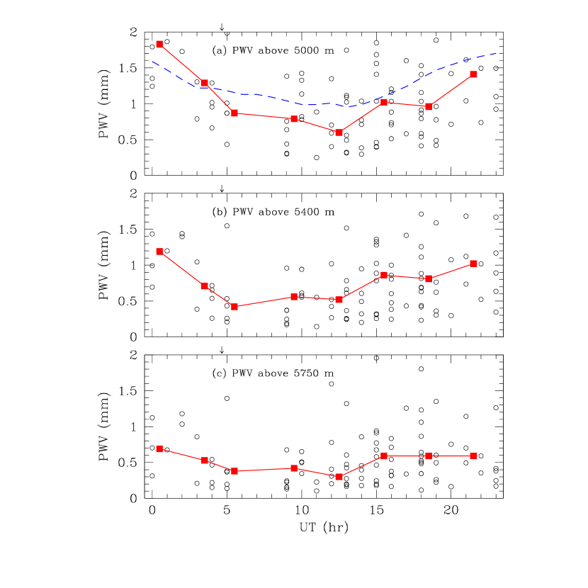
Figure 1: PWV as obtained from radiosonde profiles. The water vapor density is integrated repsectively above 5000 m, above 5400 m and above 5750 m. Unfilled circles refer to individual sonde profiles, filled squares are running medians over 3 hr intervals. Midnight is at 4:31 h UT, as indicated by the vertical arrow on top of each panel.

The diurnal cycle also affects PWV, which tends to be higher in the afternoon hours, followed by a rapid decrease after sunset. Figure 1  displays the diurnal variation of PWV above 5000 m, above 5400 m and above 5750 m, respectively top to bottom, as derived from radiosonde data (unfilled circles). Median values over 3 hr intervals are indicated as large, filled squares, connected by a solid line. The dashed line displays the median values of PWV, as obtained from 225 GHz opacities at 5000 m. Local midnight takes place at 04:31 UT. The atmosphere appears to be driest in the late part of the night and early part of the morning. The diurnal cycle of PWV lags in phase the sunlight cycle by about 4 hours, and has amplitude of about 20% about the median value.

4 Vertical Distribution of Precipitable Water Vapor

Table 1  displays quartile values of PWV above 5000, 5400 and 5750 m for four different groupings of the radiosonde flights: in addition to the daytime and nighttime sets described in Section 2, we also use the combined set of 108 sondes (“All”) and that of 32 sondes launched between UT 05 and UT 13 hrs. The latter corresponds to the UT interval in which the minimum of the diurnal cycle is seen. We note that with respect to the value of PWV at the plateau level overall, PWV drops by 30% in the first 400 m, and by a factor of 2 in the first 750 m above the plateau. That decrease may be even steeper during nighttime hours, suggesting that the effective thickness of the water vapor layer decreases at night. While the absolute values of PWV listed in Table 1 may be lower than historical values, as indicated by the comparison with 225 GHz opacities and discussed in the preceding Section, the variation of PWV with elevation is reliable.

Whether the decrease in PWV with height will be that of the free atmosphere indicated in Table 1, or lower, will depend on the local topography, the area of the summits, the direction of the wind and other factors. However, it is clear that by accessing higher ground above the plateau, significant gains in terms of infrared transparency and background emission can be obtained.

The thickness of the water vapor layer can be measured by $h_{e}$ or $h_{1/2}$. For the set of 108 radiosondes, we find the following quartile values:

$h_{1/2}$	:	571,	836,	1083	m
$h_{e}$	:	836,	1135,	1504	m

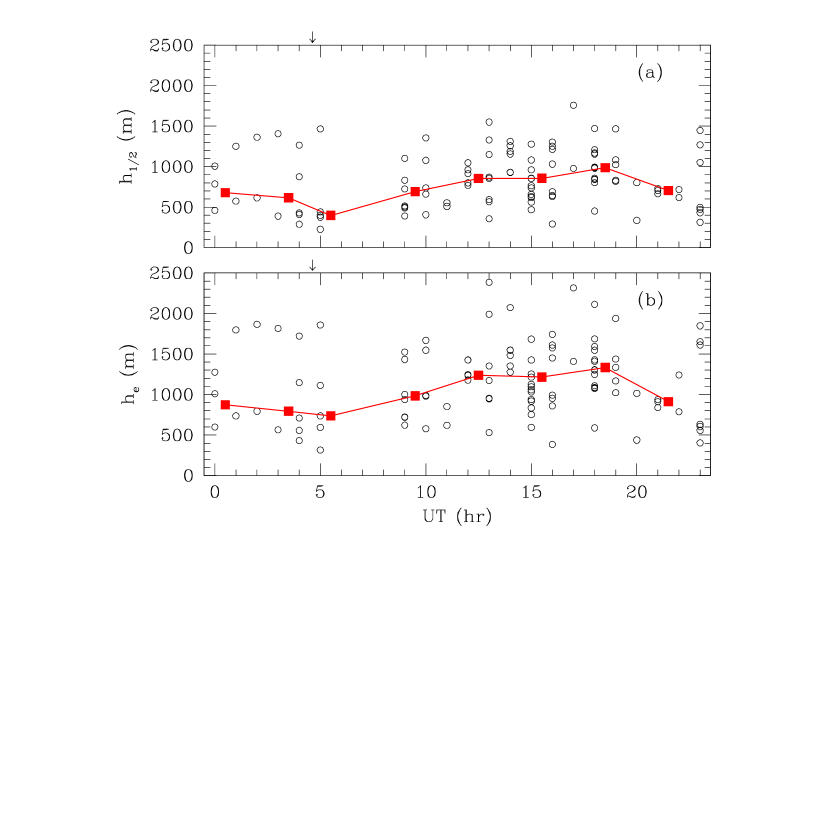
Figure 2: Half–thickness and scaleheight of the water vapor layer, as obtained from radiosonde profiles. Unfilled circles refer to individual sonde profiles, filled squares are running medians over 3 hr intervals. Midnight is at 4:31 h UT, as indicated by the vertical arrow on top of each panel.

Examining the relative humidity records from stations at different elevations at the Japanese testing site of Rio Frio, a region to the south of the Chajnantor Plateau, Holdaway et al.  (1996) found indications that the scaleheight of the water vapor layer may vary with the diurnal cycle, between values of approximately 2 and 1 km, the low value being attained at night. Figure 2  yields support for that suggestion. Values of $h_{e}$ and $h_{1/2}$ for each in the set of 108 radiosonde flights are displayed against time of day. Median values are identified by large filled squares. A diurnal oscillation in the thickness of the water layer, of amplitude near 25% about its median value, may be present. The cycle appears to be in phase with that of the solar illumination cycle. The statistical significance of this result is low, the lack of sonde launches between UT 04 and 09 hrs being particularly important in this respect. We next present corroborating evidence regarding this potentially important result.

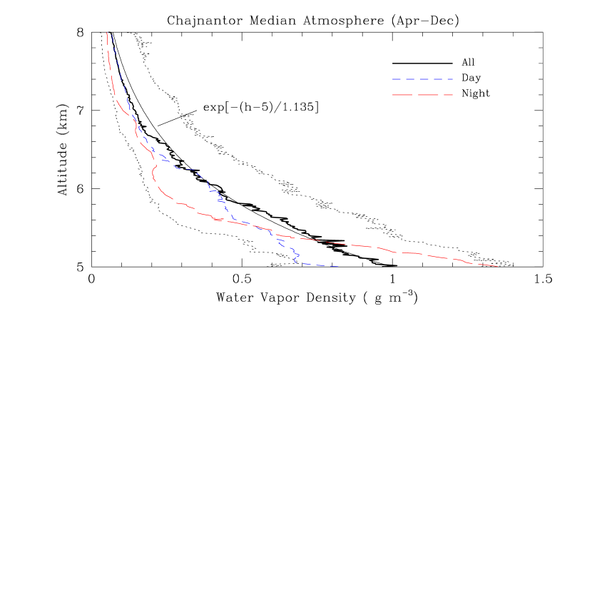
Figure 3: Distribution of the water vapor density in the median atmosphere over the Chajnantor Plateau. The thick, solid line tracks the median water vapor density, at each altitude, from 108 radiosonde profiles; the dotted lines indicate the 25% and 75% quartiles about that median. The thin solid line is an exponential of scaleheight 1.135 km. The short–dash line is the median profile for 65 daytime sondes, while the long–dash line is the median profile for 30 nighttime sondes. Note that the number of night plus day sondes is less than the total, which includes also twilight launches.

In Figure 3  we show the vertical distribution of the water vapor density in the Chajnantor median atmosphere (similar plots for the temperature distribution and the wind speed are shown in Paper I). The thick solid line tracks the median water vapor density profile over the plateau between April and December, from 108 radiosonde profiles. The distribution is well approximated by an exponential with scaleheight $h_{e}=1.135$ km, as discussed above. The median profiles for day and night radiosonde launches do however depart significantly from exponential behavior: during night, more water vapor is found at lower elevations, i.e. the effective thickness of the water layer decreases. As pointed out in teh previous section, median PWV between UT 01 hr and 11 hr (night) is about the same as between UT 12 hr and 21 hr (day), although the median value between UT 05 hr and 13 hr is significantly lower.

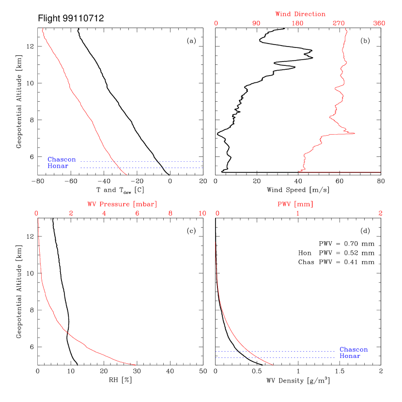
Figure 4: Radiosonde atmospheric profiles. Panels display: at upper left, temperature (thick) and dewpoint temperature; at upper right, wind speed (thick) and direction; at lower left, relative humidity (thick) and water vapor pressure; at lower right, water vapor density (thick) and PWV. The horizontal dotted lines are at the elevations of Cerro Honar (5400 m) and Cerro Chascón (5750 m). Unusually smooth atmospheric conditions are sampled by this sonde flight of 7 November 1999, UT 12 hr. No strong temperature inversions are seen in the lower atmosphere.

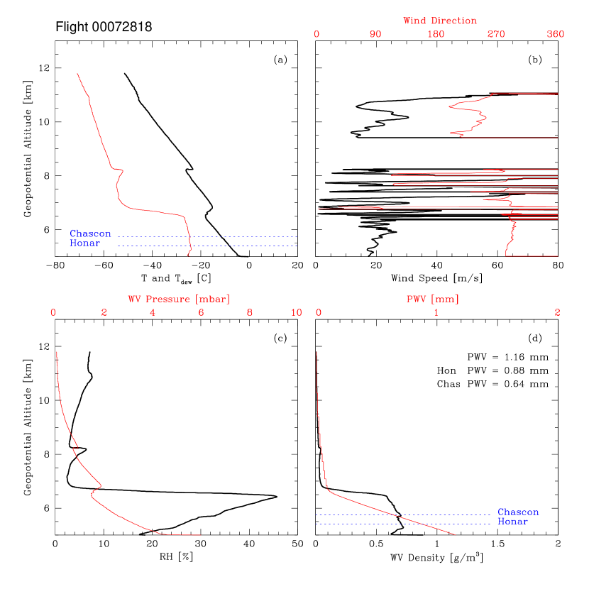
Figure 5: Radiosonde data for a 28 July 2000 launch, UT 18 hr. It shows temperature inversions near 6.6 and 8.2 km. Notice also the large increase in humidity below the 6.6 km inversion layer. Raggedness of wind data due to poor sonde tracking. Panel description as in Figure 4.

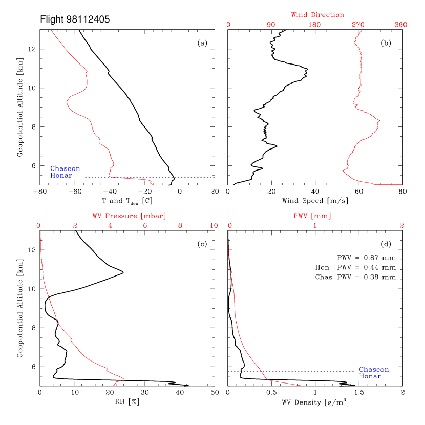
Figure 6: Radiosonde data for a 24 November 1998 launch, UT 05 hr. It shows temperature inversion below 5.4 km. Panel description as in Figure 4.

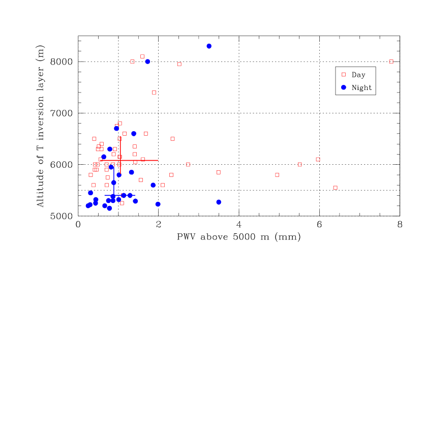
Figure 7: Altitude of temperature inversion layers identified in daytime (unfilled squares) and nighttime (filled circles) radiosonde profiles. The large crosses are plotted at the median values of elevation and PWV; the span of the crosses’ arm extend from first to third quartile.

On any given time, the departures of the water vapor distribution from an exponential can be quite severe. Figures 4, 5  and 6  display data for three different radiosonde launches. In panel (a) of each figure, the air temperature and the dewpoint temperature are displayed; in panel (b), wind speed and direction are shown; in panel (c), the relative humidity and the water vapor pressure are given, while in panel (d) we have the water vapor density and PWV. The temperature and water vapor profiles of Figure 4  are unusually smooth. The water vapor density distribution appears exponential, with a scaleheight of about 1420 m. Profiles such as that tend to be the exception. More often, temperature inversions are present, and the water vapor distribution is raggedly uneven. In the case of Figure 5, for example, two prominent temperature inversions take place near altitudes of 6600 and 8200 m. The atmospheric water vapor lies mostly under the lower of the two inversion layers, and the vertical distribution of the water vapor density is far from exponential in shape. In Figure 6, an inversion layer is present near 5300 m, and half of all water vapor above the Chajnantor Plateau is packed in the lowest 400 m of atmosphere. Were circumstances such as that displayed in Figure 6  frequent, peaks that rise several hundred m above the plateau would be highly attractive candidate sites for infrared observations. We have reviewed all radiosonde profiles and selected those for which temperature inversion layers can be identified. In Figure 7, we plot the altitude of the lowest (in case that more than one is discernible) inversion visible in the temperature profile, separately for day and night radiosonde flights. The fraction of temperature inversions taking place below 500 m above the plateau level is far larger during the night than during the day, by an amply significant margin. The nightly decrease in the thickness of the water vapor layer appears to be related to the development of temperature inversions close to the ground.

The occurrence and altitude of temperature inversions is of importance not only for their impact on the PWV, and thus the infrared transparency, of a site, but also for the quality of astronomical seeing. Evidence exists (Hufnagel 1978) that in those layers large values of the refractive index structure constant $C_{n}^{2}$ occur. The seeing disk of stellar images, $\theta_{hpfw}\propto\int C_{n}^{2}dz$, can thus be strongly affected. A site above the inversion layer would hence yield better astronomical image quality.

5 Atmospheric Transparency in the Infrared

5.1 Atmospheric Transparency and Thermal Background

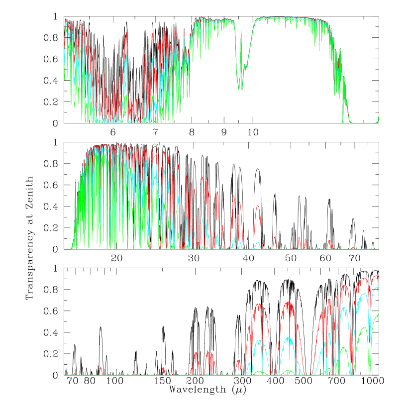
Figure 8: Atmospheric transparency at zenith between 5 and 1000 $\mu$m, for a site at an altitude of 5000 m and different H₂O column densities: the tracings, top to bottom, correspond to 0.1, 0.4, 1.0 and 3.0 mm of PWV.

Figure 8  displays curves of atmospheric transparency at zenith, computed for a site at an altitude of 5000 m and different column densities of water vapor above head, for the window between 5 $\mu$m and 1 mm. In the spectral region between 50 and 200 $\mu$m the atmosphere is quite opaque from all ground sites: even if PWV were as low as 100 $\mu$m, transparency would not reach 40%. However, the window near 200 $\mu$m may be of interest for observations of the very important spectral line of $C^{+}$. For low values of PWV, numerous atmospheric windows appear longwards of 10 $\mu$m, notably near 20, 24, 32, 34, 38, 42 and 46 $\mu$m.

The main deleterious effects of the atmosphere on astronomy consist in reduced transparency to cosmic photons from a given line of sight, seeing degradation of optical and infrared images and an increase of the diffuse background, against which the generally weak signals of cosmic sources need to be discriminated. The effective temperature of the most relevant atmospheric layers is between 200 and 300 K, so the atmospheric thermal emission peaks near 15 $\mu$m. Near the centers of the absorption bands where the atmosphere is opaque, a maximum background flux is reached and, of course, no cosmic photons get through. In spectral regions of partial transparency, the atmospheric background radiation can be approximated by that of a blackbody attenuated by a factor which is the complement of the transparency. If opacity is distributed over a wide range of elevations, this assumption may be flawed; it is however a good approximation for the opacity produced by water vapor, which is found very close to the ground, and is our main concern in this paper. In the optical and near IR, the principal source of atmospheric background is the scattering of solar radiation, during the day. At night, however, airglow in the near IR results from transitions between vibrational states of the OH^- radical, discharging energy stored during daytime from solar radiation, through the dissociation of ozone. Thus OH^- airglow originates at heights of 70 to 90 km and affects all ground based locations, independently on altitude.

In addition to the atmospheric background, astronomical observations need to contend with cosmic backgrounds, such as that produced by the thermal emission and the scattering of solar photons by interplanetary dust, the interstellar dust emission, the cosmological microwave background radiation and the thermal emission of the telescope and detectors themselves.

We next compute background levels for various atmospheric conditions; in doing so we follow the approach of Thronson et al. (1995).

Let’s first consider the “near field” thermal background. In the atmospheric windows of interest the atmosphere is optically thin, so that the specific intensity of the emitted radiation can be approximated by

$$I_{\nu}=\tau_{\nu}B_{\nu}={2\tau_{\nu}(h\nu^{3}/c^{2})\over exp(h\nu/kT)-1}$$ (2)

where $B_{\nu}$ is Planck’s function and $\tau_{\nu}$ the optical depth. Thus the number of photons per unit time. originating with the thermal background of temperature $T$ and striking the telescope within the solid angle subtended by a point source $\Omega_{ps}$, is

$${\cal\char 66\relax}=I_{\nu}~{}{\cal\char 65\relax}~{}\Omega_{ps}\Delta\nu/h\nu$$ (3)

where ${\cal\char 65\relax}$ is the collecting area of the telescope and $\Delta\nu$ is the detection bandwidth. Converting to photoelectrons per second and assuming a detector gain of 1

$${\cal\char 66\relax}_{e}=2.22\times 10^{15}~{}{{\cal\char 84\relax}~{}QE\over\cal\char 82\relax}{{1-e^{-\tau}}\over\lambda_{\mu}[exp(1.44\times 10^{4}/\lambda_{\mu}T)-1]}~{}~{}~{}~{}~{}{\rm[e~{}~{}s^{-1}]}$$ (4)

where ${\cal\char 84\relax}$ and $QE$ are respectively the system transmission and quantum efficiency over the band, $\lambda_{\mu}$ the wavelength in $\mu$m, and ${\cal\char 82\relax}$$=\nu/\Delta\nu=\lambda/\Delta\lambda$. Equation  4 is derived assuming that the telescope is diffraction limited at all wavelengths, so that $\Omega_{ps}$ is the solid angle subtended by the ring corresponding to the first diffraction null and ${\cal\char 65\relax}\Omega_{ps}$ is then $3.7\lambda_{\mu}^{2}$. This assumption makes the background estimate independent on telescope aperture, allowing an intercomparison of different sites or atmospheric conditions. At the shorter wavelengths, at which the seeing angle is larger than the diffraction limit of the aperture, such an assumption is incorrect, and $\Omega_{ps}$ should be replaced with the solid angle which encircles 90% of the light within the seeing disk.

Different sources of thermal emission yield an additive contribution to ${\cal\char 66\relax}_{e}$. For the atmospheric thermal background, we approximate $\tau$ with the complement to one of the transparency as displayed in Figure 8. For the thermal emission of the telescope, we replace $\tau$ in Eqn. 4  with a constant emissivity $\epsilon_{tel}$.

As for the cosmic backgrounds, following Tokunaga (1998) and using Equation  4, we approximate the zodiacal emission of dust by that of a blackbody with $T=275$ K attenuated by $\epsilon=7.1\times 10^{-8}$; the sunlight scattered by the interplanetary particles by a blackbody of $T=5800$ K and $\epsilon=3\times 10^{-14}$; the interstellar dust emission by a blackbody of $T=17$ K and $\epsilon=10^{-3}$; and the cosmic microwave background by a blackbody with $T=2.73$ K and $\epsilon=1$.

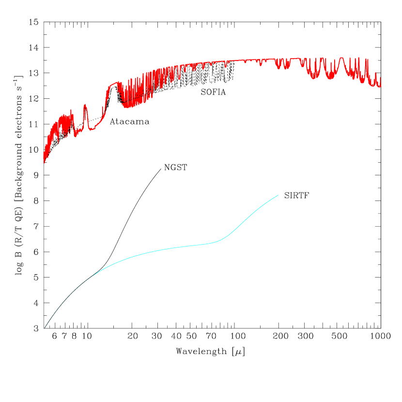
Figure 9: The total backgrounds for Atacama (very best atmospheric conditions with PWV=0.2 mm and seeing FWHM of 0.35” at 0.5 $\mu$m assumed) and several space and airborne telescopes are compared. Note that that ${{\cal\char 84\relax}}~{}QE/{\cal\char 82\relax}\simeq 1$. See text for further details.

Figure 9  illustrates the background ${\cal\char 66\relax}_{e}$ for an Atacama telescope with $\epsilon_{tel}=0.05$, estimated for the very best atmospheric conditions of $PWV=0.2$ mm and a seeing of 0.35” at 0.5 $\mu$m(as shown in Table 1, PWV=0.2 mm is the value for the lowest quartile at a high elevation site, and seeing near 0.35” may have similar frequency at such a site; the chosen combination of values may occur in 5–20% of the time, depending on how correlated seeing and PWV are; of eight reliable events of simultaneous radiosonde and seeing measurements, the four with PWV$<1$ mm yield an average seeing of 0.51” at 0.5 $\mu$m, while the other four, with PWV$>1$ mm, have average seeing of 0.84”; more data is needed to confirm this possible correlation). In the same figure, we also display estimates of the background for a space telescope passively cooled (e.g. the Next Generation Space Telescope, NGST), a cryogenically cooled space telescope (e.g. the Space Infrared Telescope Facility, SIRTF), and a stratospheric, telescope airborne at 12 km altitude (above which PWV is assumed to be 10 $\mu$m, $\epsilon_{tel}=0.15$, and image quality of 2” at 1 $\mu$mfor SOFIA (this may be an overestimate of image quality: while the optical quality of the instrument is high, pointing jitter and seeing produced by the turbulent air flow near the airplane may produce worse values). We have assumed a telescope temperature of 260 K for Atacama, 240 K for SOFIA, 60 K for NGST and 5.5 K for SIRTF. The temperature of the emitting atmospheric layers was assumed to be 255 K for Atacama and 230 K for SOFIA. For simplicity, we assume ${{\cal\char 84\relax}}\cdot QE\cdot G/{\cal\char 82\relax}=1$, which overestimates the bandwidths that are possible in some of the atmospheric windows. Telescope and atmospheric thermal backgrounds dominate in the case of all ground–based instruments, while in the case of space instruments, even if not cryogenically cooled, the zodiacal emission dominates. Between 5 and 15 $\mu$m, for example, the NGST will have a background about six orders of magnitude lower than that for an Atacama telescope. While airborne at high altitude, the SOFIA telescope itself will produce substantial thermal emission, and lower image quality than can be achieved from the ground. Note that the background in good Atacama conditions and for Sofia are comparable. SOFIA will, however, have access to atmospheric windows inaccessible from the ground.

5.2 Comparison of Broad Band Sensitivities

The signal–to–noise ratio ${\cal\char 81\relax}$  for a single integration of time $t$ can in general be expressed as (Thronson et al. 1995)

$${\cal\char 81\relax}={{\cal\char 83\relax}~{}t\over[({\cal\char 83\relax}+{\cal\char 66\relax}_{e}+{\cal\char 68\relax})t+R^{2}+N_{c}t^{2}]^{1/2}}$$ (5)

where ${\cal\char 83\relax}$ is the source signal, ${\cal\char 68\relax}$ is the detector dark current, $R$ its readout noise and $N_{c}$ is the signal produced by source confusion. A given signal, such as $S$, relates to the flux density via

$${\bf S}({\rm mJy})e^{-\tau}=6.63\times 10^{-5}{{\cal\char 82\relax}\over QE~{}{{\cal\char 84\relax}~{}{\cal\char 65\relax}}}~{}{\cal\char 83\relax}$$ (6)

We adopt the following detector performance characteristics for the 3–40 $\mu$m  range: $QE\simeq 0.50$, ${\cal\char 68\relax}\simeq 10$ $e^{-}s^{-1}$ and $R\simeq 50$ electrons rms (Thronson et al. 1995; Stacey 2000; Brandl & Pirger 2000), and source confusion does not become an issue shortwards of 50 $\mu$m, as we shall discuss in the next Section. It is thus safe to assume that in the near and mid–IR the thermal background dominates for broad band observations, so that the minimum detectable signal, for an exposure of time $t$ achieving signal–to–noise ${\cal\char 81\relax}$, according to Equation 5  is

$${\cal\char 83\relax}_{min}\simeq{\cal\char 81\relax}~{}[{\cal\char 66\relax}_{e}/t]^{1/2}.$$ (7)

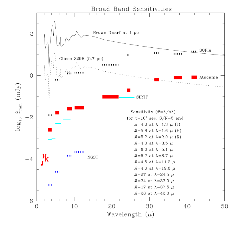
Figure 10: Comparison of sensitivities for several proposed or future telescopes, for a signal–to–noise ratio of 5 and an integration of 10⁴ s. The length of the horizontal bars identifying each waveband illustrates ${\cal\char 82\relax}$ as tabulated in the inset. See text for assumed telescope parameters. The 15 m Atacama telescope is assumed seeing limited with image size of 0.35”. The labels ‘J’, ‘H’ and ‘K’ refer to the Atacama sensitivities. The J band limit is equivalent to about 26th magnitude. For reference, the spectral shape of a brown dwarf (Gliese 229B) has been plotted at the assumed distances of 1 and 5.7 pc. One mJy is $10^{-29}$ W m^-2 Hz^-1.

We use Equations 4  and 7  to estimate limiting fluxes for point sources, assuming ${\cal\char 84\relax}$$=0.4$ and, as indicated above, $QE=0.5$. The broadest bandwidths usable are, of course, limited by atmospheric absorption. Sensitivities are computed for ${\cal\char 81\relax}=5$ and exposures of $t=10^{4}$ sec. We underscore the fact that the chosen bands are those accessible from the ground: SOFIA, SIRTF and NGST will access spectral regions inaccessible from the ground. The results are plotted in Figure 10, for a telescope at Atacama with a 15 m diameter, NGST of 6 m diameter, SIRTF with a 0.85 m diameter and SOFIA with a diameter of 2.4 m. In the case of the Atacama telescope, we have assumed that the image size is seeing–limited at 0.35” at 0.5 $\mu$m. Note that with an adaptive optics system of moderate to good efficiency, the near infrared sensitivity can improve by one order of magnitude, beyond the limit in Figure 10, provided that it does not significantly increase the telescope emissivity. The implementation of an adaptive secondary would thus be desirable and that of a multiconjugate system would raise more serious emissivity concerns. The point source sensitivity plotted in Figure 10  for J band is equivalent to 26th magnitude; with an AO system that limit would approach 29th magnitude. The telescope labels are the same as for Figure 9. The SIRTF sensitivities have been obtained from the SIRTF website (http://ssc.ipac.caltech.edu/sirtf/Mission) and links referred therein. The NGST sensitivities have been plotted for the same bandpasses and ${\cal\char 82\relax}$ as for the Atacama telescope, although it should be clear that the whole near IR spectrum will be accessible to NGST. For comparison, we also plot the flux density curves of the brown dwarf Gliese 229B at the source’s distance of 5.7 pc and at 1 pc (Matthews et al. 1996).

The thermal background does not always constitute the main limitation at submillimeter wavelengths. Source confusion can become important. The sky source density at far IR and submm wavelengths is relatively uncertain, but it is unlikely to be a concern even for large integrations ($\sim 10^{4}$ s) for large aperture telescopes (diameter greater than 10 m). Assuming ${{\cal\char 84\relax}}=0.4$, $QE=0.5$ (a quantum efficiency which can be approached by detectors with modern bolometers) and optimal atmospheric conditions as can be found in Atacama (PWV=0.2 mm), an observation with Q$=5$ and $t=10^{4}$ s can reach a sensitivity on the order of 1 mJy at all the atmospheric windows between 300 $\mu$m and 1 mm, and about 3 mJy for those between 200 and 300 $\mu$m.

5.3 Comparison of Spectroscopic Sensitivities

Suppose the flux density contributed at a given frequency by a spectral line is S. The integrated flux over the whole line is $\int Sd\lambda$. If the spectral line is unresolved, the flux associated with the line is $S\Delta\lambda=S\lambda/\cal\char 82\relax$, where S is now the mean line flux over the spectral channel which contains the line. If we measure the integrated flux in W m^-2, then the signal $S$ in electrons per second can be converted to

$$F{\rm(W~{}m}^{-2})=2.0\times 10^{-19}{S\over\lambda_{\mu}~{}A~{}QE~{}{\cal\char 84\relax}}$$ (8)

In spectroscopic observations, the high ${\cal\char 82\relax}$ reduces the impact of the high thermal background, as illustrated by Equation  4. For observations with ${\cal\char 82\relax}$$=10^{5}$, for example, the thermal background contribution, which is inversely proportional to ${\cal\char 82\relax}$, will be several orders of magnitude lower than in the case of photometric observations. Consider Equation  5: ${\cal\char 66\relax}_{e}$ can become comparable with or smaller than ${\cal\char 68\relax}$, in which case the observation will be limited by detector noise. For values of ${\cal\char 68\relax}\simeq 10$ e^- s^-1 and $R\simeq 50$ electrons, the background can easily become negligible with respect to ${\cal\char 68\relax}$ in space–based instruments. The readout noise on the other hand is likely not to play a role if exposures exceed a few hundred seconds, because then $R^{2}<{\cal\char 68\relax}t$. We will assume here that $R^{2}$ and the source confusion term in the denominator of Equation 5  are negligible.

The minimum detectable integrated line flux for an integration time $t$, with a signal–to–noise ratio ${\cal\char 81\relax}$, can be written, in analogy to Equation 7, as

$$F_{min}{\rm(W~{}m}^{-2})=2.0\times 10^{-19}{{\cal\char 81\relax}\over\lambda_{\mu}~{}A~{}QE~{}{\cal\char 84\relax}}~{}\Bigl{[}{{\cal\char 66\relax}^{\prime}\over t}\Bigr{]}^{1/2}$$ (9)

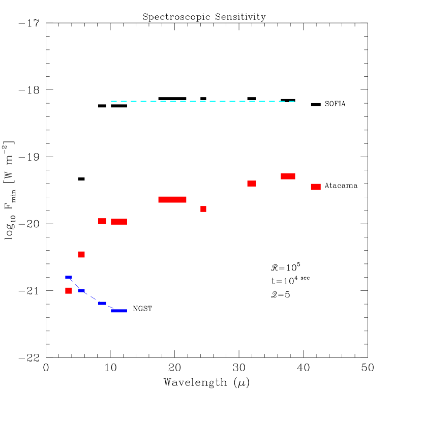
Figure 11: Spectral sensitivities for several proposed telescopes; for Atacama, calculations correspond to ${\cal\char 82\relax}$$=10^{5}$, ${\cal\char 81\relax}=5$ and $t=10^{4}$ sec. The spectral sensitivity of SIRTF, at its highest resolution of 600, is indicated for comparison by a horizontal dashed line.

where ${\cal\char 66\relax}^{\prime}$ is ${\cal\char 66\relax}_{e}+{\cal\char 68\relax}$. Note that, for a space–based instrument, near 5 $\mu$m ${\cal\char 66\relax}_{e}\simeq 5\times 10^{-3}$ e^- s^-1 for ${\cal\char 82\relax}$$=10^{5}$, so ${\cal\char 66\relax}_{e}\ll{\cal\char 68\relax}$, and the instrument is detector–limited. In Figure 11, we show sensitivity limits computed using Equation  9, for ${\cal\char 82\relax}$$=10^{5}$, ${\cal\char 68\relax}$=10, $QE=0.5$, ${\cal\char 84\relax}$=0.4 and ${\cal\char 81\relax}$=5, except for SIRTF, for which ${\cal\char 82\relax}$ is only 600.

6 Conclusions

The water vapor distribution above the Chajnantor plateau appears to have the following properties:

• The median PWV above the plateau at 5000 m is $\sim 1.2$ mm. Variations from year to year can be as large as 50% of that value.

• Seasonal variations in PWV are also large: median values for the 8 months from April to November are 30% lower than the yearly median, while median values for the Summer months may be more than twice as large.

• PWV varies by about $\pm 20$% with the daily cycle, with a phase lag about 4 hours behind that of sunlight: minimum PWV occurs between midnight and noon, and maximum occurs at sunset.

• The distribution of the water vapor of the median atmosphere over Chajnantor is well aproximated by an exponential, with a scaleheight of 1.13 km. At any given time, however, the water vapor distribution can depart from an exponential shape, more dramatically when temperature inversions occur.

• The thickness of the water vapor layer appears to vary in phase with the solar illumination cycle by about $\pm 25$%; minimum is near local midnight.

The implications of these effects for summits in the vicinity of the Chajnantor Plateau are:

• The median PWV above 5400 m elevation drops by one third with respect to the value measured at the plateau; above an elevation of 5750 m it drops by a factor of 2.

• Median PWV in winter nights at a summit near 5400 m, such as Cerro Honar, may be as low as 0.5–0.6 mm, if conditions near the summit approach those of the free atmosphere. The lowest quartile of PWV may approximate 0.35–0.40 mm.

• Median PWV in winter nights at a summit near 5700 m, such as Cerro Chascón may approximate 0.40 mm, and the lowest quartile near 0.20–0.25 mm.

• Low elevation temperature inversions are more likely during nighttime. During those episodes, much of the PWV is trapped below the inversion layer, and mountain peaks are offered a nearly dry atmosphere, possibly endowed with high quality seeing.

The conclusions listed above rely on still relatively sparse data from 108 radiosondes and should be considered as preliminary. However, these results suggest that exceptional possibilities for ground–based IR and submm astronomical observations exist in the Llano de Chajnantor region. The combination of low water vapor content and high quality seeing allow for low atmospheric background in the near and mid–IR. At a telescope on a summit in the vicinity of the Chajnantor plateau, numerous atmospheric windows would appear in the mid IR, up to about 50 $\mu$m. In the far IR and submillimeter regime, the 350 $\mu$m, 450 $\mu$m, 600 $\mu$m, 750 $\mu$m and 870 $\mu$m windows reach exceptional transparency, while two useful windows appear near 200 $\mu$m. Broad band observations with a 15 m class telescope at such a site would be close in sensitivity to those made with SIRTF in the mid–IR, offering a superb synergy match for follow–up observations of the SIRTF surveys. The near and mid–IR performance of such a ground–based telescope in high resolution spectroscopic mode would be exceptional and could only be exceeded by that of a space telescope of comparable aperture. The relative ease and cost–effectiveness of operation in the Atacama advises that serious attention be given to the Atacama sites for the installation of the next generation of large infrared telescopes.

Acknowledgements: The support and assistance of Joe Veverka, Yervant Terzian, Bob Richardson, Jennifer Yu and Bryan Isacks of Cornell U.; Martha Haynes of Cornell U. and Associated Universitites, Inc.; Robert L. Brown, Eduardo Hardy and Geraldo Valladares of NRAO; the use of radiosonde data obtained through a collaboration with NRAO (Simon Radford and Bryan Butler), ESO (Angel Otarola) and SAO (Ray Blundell and Scott Paine); access to 225 MHz radiometry data of NRAO (Simon Radford); don Tomás Poblete Alay and the staff of La Casa de Don Tomás are thankfully acknowledged. This study was made possible by a grant of the Provost’s Office of Cornell University and the National Science Foundation grant AST–9910136.

Table 1: PWV (mm) Quartiles for 108 Radiosondes.

Quartile	5000 m	5400 m	5750 m	N
All	—	—	—	108
25%	0.71	0.40	0.27
50%	1.04	0.72	0.49
75%	1.75	1.28	0.92
Day	—	—	—	65
25%	0.58	0.40	0.32
50%	1.04	0.82	0.54
75%	1.75	1.33	1.00
Night	—	—	—	30
25%	0.76	0.37	0.21
50%	1.00	0.57	0.42
75%	1.42	1.05	0.68
UT 05–13	—	—	—	32
25%	0.46	0.26	0.20
50%	0.85	0.53	0.36
75%	1.23	0.86	0.63

References

- (1) Brandl, B. & Pirger, B. 2000, personal communication
- (2) Delgado, G., Otarola, A., Belitsky, V. & Urbain, D. 1999, preprint
- (3) Giovanelli, R., Darling, J., Sarazin, M., Yu, J., Harvey, P., Henderson, C., Hoffman, W., Keller, L., Barry, D., Cordes J., Eikenberry, S., Gull, G., Harrington, J., Smith, J.D., Stacey & G., Swain, M. 2000, submitted (Paper I)
- (4) Holdaway, M.A., Ishiguro, M., Nakai, N. & Matsushita, S. 1996, MMA Memo nr. 158, NRAO:Tucson
- (5) Holdaway, M.A., Ishiguro, M., Foster, S., Kawabe, K., Kohno, K., Radford, S. & Saito, M. 1996, MMA Memo nr. 152, NRAO:Tucson
- (6) Hufnagel, R.E. 1978, in The Infrared Handbook, ed. by W.L. Wolfe & G.J. Zissis (U.S. Govt. Printing Office: Washington, D.C.), Chapter 6.
- (7) Matthews, K., Nakajima, T., Kulkarni, S.R. & Oppenheimer, B.R. 1996, AJ 112, 1678.
- (8) McPhaden, M.J. 1999, Science 283, 950
- (9) Otarola, A. 2000, in http://puppis.ls.eso.org/lsa/lsahome.html
- (10) Radford, S. 2000, in http://www.tuc.nrao.edu/mma/sites/Chajnantor
- (11) Stacey, G. 2000, personal communication
- (12) Thronson, Jr., H.A, Rapp, D., Bailey, B, & Hawarden, T.G. 1995, PASP 107, 1099.
- (13) Tokunaga, A.T. 1998, in Astrophysical Quantities, 4th edition, editor A. Cox, Springer–Verlag, in press.
- (14) Wolfe, W.L. & Zissis, G.J. 1978, The Infrared Handbook, Office of Naval Research, Dept. of the Navy, Washington, D.C.