Limits Due to Instrumental Polarisation in CMB Experiments at Microwave Wavelengths

Abstract

An extended analysis of some instrumental polarisation sources has been done, as a consequence of the renewed interest in extremely sensitive polarisation measurements stimulated by Cosmic Microwave Background experiments. The case of correlation polarimeters, being them more suitable than other configurations, has been studied in detail and the algorithm has been derived to calculate their intrinsic sensitivity limit due to device characteristics as well as to the operating environment. The atmosphere emission, even though totally unpolarised, has been recognized to be the most important source of sensitivity degradation for ground based experiments. This happens through receiver component losses (mainly in the OMT), which generate instrumental polarisation in genuinely uncorrelated signals. The relevant result is that, also in best conditions (cfr. Antarctica), integration times longer than $\sim 40$ s are not allowed on ground without modulation techniques. Finally, basic rules to estimate the maximum modulation period for each instrumental configuration have been provided.

1 Introduction

The Cosmic Microwave Background (CMB), which has a black–body (BB) spectrum at a thermodynamic temperature $T_{\rm o}=2.728$K (Fixsen et al., 1996), is a powerful tool to understand origin and evolution of our universe. The CMB looks almost isotropic and unpolarised and any detection of deviations from an ideal BB would be very important because they allow the estimate of cosmological parameters (Jungman et al. 1996, Zaldarriaga et al. 1997, Efstathiou & Bond 1999). Very small temperature fluctuations in the CMB have been detected at both large (Smooth et al. 1991, Bennet et al. 1996) and small (De Bernardis et al. 2000, Hanany et al. 2000, Miller et al. 1999) angular scales, but only upper limits on the CMB polarisation (CMBP) have been evaluated (Hedman et al. 2000 and see Staggs et al. 1999 for a complete list of the CMB polarisation measurements).

The analysis of the linearly polarised component of the CMB promises to be very important in the cosmological frame. In fact, the CMBP can solve the degeneracies among cosmological parameters that CMB anisotropy alone is not able to remove (Zaldarriaga et al. 1997). Moreover, it allows the separation of scalar and tensorial components of the primordial fluctuations providing a way to disentangle among different inflationary models (Kamionkowski & Kosowsky 1998).

Several microwave experiments, based on radiometric receivers, are either operating or planned to search for the CMB linear polarisation at both large and small angular scales, either from ground or from space. SPOrt (Cortiglioni et al. 1999), the Milano Polarimeter (Sironi et al. 1998) and POLAR (Keating et al. 1998) will operate at $7^{\rm o}$ scale by using simple optics; PIQUE (Hedman et al., 2000) will investigate angular scales below $1^{\rm o}$ by means of mirror optics. Both MAP (Bennet et al. 1997, Wright 1999) and Planck–LFI (Tauber, 2000), even though they do not have polarimeters on board, will also try to derive CMBP information at subdegree angular scale. For all of them the expected signal level is low: on $7^{\rm o}$ scale the polarised emission can be lower than 1 $\mu$K, while on smaller angular scales ($<1^{\rm o}$) signals can be of the order of few $\mu$K.

Moreover, it is well known that CMB experiments have to deal with Galactic contribution removal. In fact, the Galactic background beside its intrinsic interest, acts as a foreground for CMB experiments and only its accurate knowledge will allow detections of the CMB features (Brandt et al. 1994, Dodelson 1997, Bouchet et al. 1999, Tegmark et al 2000, Prunet et al. 1998, Kogut & Hinshaw 2000, Tucci et al. 2000a, Baccigalupi et al. 2000). Our Galaxy is featured by a smoothed linearly polarised background emission, carrying information on the Galactic structure, that has been observed at frequencies up to 2.7 GHz (Brouw & Spoelstra 1976, Junkes et al. 1987, Duncan et al. 1999, Duncan et al. 1997, Uyaniker et al. 1999, McClure-Griffiths et al. 2001, Gaensler et al. 2001), where it results to be dominated by the synchrotron emission.

No all–sky observations of polarised Galactic background have been made so far in the microwave domain, where synchrotron emission should prevails, even though it has been recently suggested that spinning and magnetic dust grain linearly polarised emission should be not negligible in the 20–70 GHz range (Draine & Lazarian 1999, Lazarian & Draine 2000, Tegmark et al. 2000). At millimeter wavelengths, saying above 100 GHz (Kogut et al. 1996), the Galactic emission is dominated by Galactic thermal dust. The expected scenario, showing that in any case the antenna temperatures to be detected are extremely low, is represented in Figure 1.

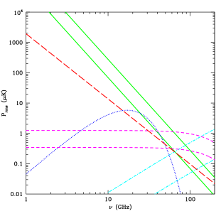
Figure 1: Plot of the expected level of polarisation emission on $7^{\rm o}$ angular scale: CMB (dashed lines: two CDM models with optical depth $\tau$=0.1–0.5, respectively), Synchrotron (solid lines: normalized to 5–20 mK at 2.4 GHz), Free–Free (long–dashed), Thermal Dust (dot–dashed lines: 5–0.5% polarised) and Spinning Dust (dotted). See Tucci et al. (2000b) for details about normalizations.

In spite of this, most of the noise in CMBP experiments would come from the CMB itself, because such experiment must detect a very weak signal (few $\mu$K or less) in presence of the strong unpolarised background $T_{\rm o}$. In addition, the instrumental noise and the atmospheric emission (for ground based experiments) contribute to the total signal collected by the instrument making stronger and variable this unpolarised (unwanted) component.

The losses of radiometer components will transform such an unpolarised part of the input signal in a so called spurious polarised component, which should be kept, in principle, lower than the genuine polarised signal to be searched (namely lower than 1 $\mu$K). Every experiment has to deal with such instrumental offsets, which are also detected as genuine polarisation, but they are not. Then, even though in certain conditions suitable scanning strategies or signal modulation techniques may allow the extraction of the true signal by post–processing data analysis (for instance cfr. Revenu et al. 2000, Carretti et al. 2000, Carretti et al. 2001), the common baseline is to keep offsets as low as possible.

However, the most important problem introduced by the offset are its fluctuations, which can strongly degrade the instrument sensitivity. The radiometer sensitivity equation may be written as (Wollack & Pospieszalski 1998, Wollack 1995):

$$\Delta T_{\rm rms}=\sqrt{{k^{2}\,T_{\rm sys}^{2}\over\Delta\nu\,\tau}+T_{\rm offset}^{2}\left({\Delta G\over G}\right)^{2}+\Delta T_{\rm offset}^{2}}$$ (1)

being $T_{\rm sys}$, $T_{\rm offset}$ and $\Delta T_{\rm offset}$ the system temperature, the offset equivalent temperature and its fluctuation, respectively; $G$ is the radiometer gain, $\tau$ the integration time, $\Delta\nu$ the radiofrequency bandwidth and $k$ a constant depending on the radiometer type. The first term represents the white noise of an ideal and stable radiometer; both the second and the third terms represent additional noise generated by instrument instabilities driven by the offset.

The main aim of this work is to analyse some usual configuration of microwave polarimeters with respect to the offset generation, to evaluate the effect on the sensitivity degradation introduced by the offset itself. This analysis considers only correlation polarimeters, which are intrinsically more stable with respect to other configurations.

2 ${\bf Q}$ and ${\bf U}$ Stokes Parameters Measurements

The polarisation status of the radiation is usually described by the Stokes parameters $I$, $Q$, $U$ and $V$ (see, for instance, Kraus 1987, Rohlfs & Wilson 2000). The linearly polarised component is fully defined by $Q$ and $U$, which give the linear polarised intensity and the polarisation angle:

$$I_{p} = \sqrt{Q^{2}+U^{2}}$$ (2)

$$\alpha = {1\over 2}\tan^{-1}(U/Q).$$ (3)

$V$ and $I$ represent the circularly polarised component and the total emission (unpolarised + polarised), respectively.

Since both the CMB and the Galactic emission are expected to be (partially) linearly polarised, with negligible circular polarisation ($V\approx 0$), this paper deals only with the $Q$ and $U$ detection.

$Q$ and $U$ Stokes parameter measurements using correlation instruments can be carried on in several ways (for instance see SPOrt, Milano Polarimeter, POLAR, PIQUE). However, all of them multiply the two signals, saying $A$ and $B$ coming from the antenna system, providing two outputs that, using a Fourier spectral representation, can be expressed as:

$$O_{1} \propto 2\,\Re(AB^{*})$$

$$O_{2} \propto 2\,\Im(AB^{*})$$ (4)

These instruments can be divided into two groups with respect to the signals to be correlated, depending on the characteristics of the antenna system. In fact, the two signals $A$ and $B$ can represent either the two circularly or the two linearly polarised components of the incoming radiation.

In the case where $A$ and $B$ are the right–hand and left–hand circularly polarised components, respectively, the two correlator outputs are proportional to $Q$ and $U$:

$$O_{1} \propto 2\,\Re(E_{R}E_{L}^{*})=Q$$

$$O_{2} \propto 2\,\Im(E_{R}E_{L}^{*})=U$$ (5)

and they provide a direct and a simultaneous measurement of the two Stokes parameters describing the linear polarisation.

Differently, if $A\propto E_{X}$ and $B\propto E_{Y}$ are the two linearly polarised components with respect to the cartesian reference frame of the instrument, the two correlator outputs are proportional to $U$ and $V$:

$$O_{1} \propto 2\,\Re(E_{X}E_{Y}^{*})=U$$

$$O_{2} \propto 2\,\Im(E_{X}E_{Y}^{*})=V$$ (6)

providing only one (U) of the two Stokes parameters needed to describe the linear polarisation. However, a rotation of the reference frame converts $Q$ into $U$ and viceversa through:

$$Q = Q_{0}\cos(2\beta)+U_{0}\sin(2\beta),$$ (7)

$$U = U_{0}\cos(2\beta)-Q_{0}\sin(2\beta),$$ (8)

where $\beta$ is the rotation angle of the antenna around its axis. In this way, the measurement of $Q$ can be done with $\beta=45^{\rm o}$, so that the two parameters can be obtained sequentially. Since this configuration does not provide simultaneously $Q$ and $U$ its time efficiency is reduced of 50% with respect to the previous configuration, where circularly polarized components are used.

3 Spurious Polarisation

In the previous section the outputs for an ideal polarimeter have been described. In real instruments the two channels $A$ and $B$ are not completed isolated. Hence, they are partially correlated also in presence of unpolarised radiation only.

Such a contamination can be generated only in common parts, that is where signals propagate together (in the same device) and they can cross each to the other. In correlation polarimeters the common parts are the antenna system as well as the correlation unit (see Figure 2).

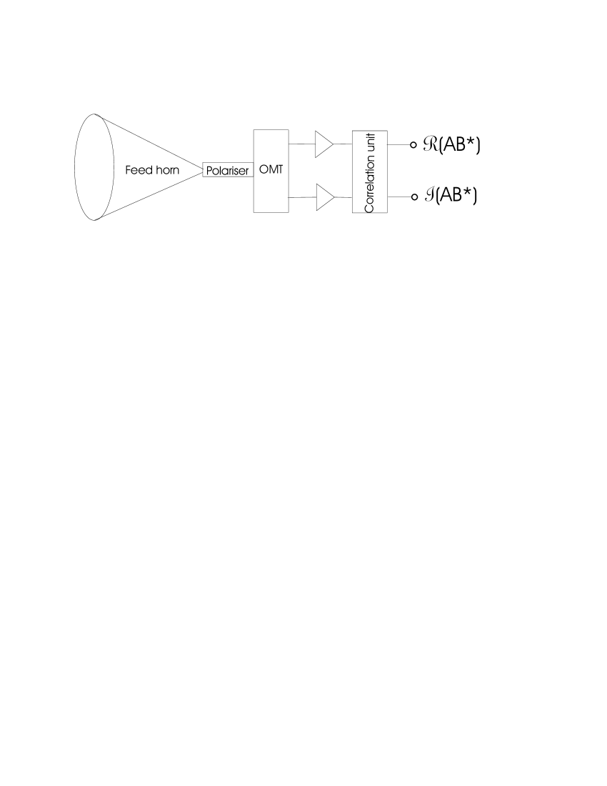
Figure 2: A correlation polarimeter can be divided in three parts. The antenna system collects the sky signal and provides the signals $A$ and $B$ (the polariser is requested only to have circularly polarised components). The amplification chain amplifies the two divided signals. Finally, the correlation unit multiply the signals and provides two outputs proportional to $\Re(AB^{*})$ and $\Im(AB^{*})$. Antenna system and correlation unit represent the common parts where $A$ and $B$ can cross–correlate.

In order to estimate how these effects can influence the measured outputs $Q^{\prime}$ and $U^{\prime}$, they will be analyzed with respect to the actual (from the sky) values of the whole Stokes parameters set ($I$, $Q$, $U$, $V$).

The contaminated signals $A^{\prime}$ and $B^{\prime}$ at the output of a device can be expressed, with respect to the ideal ones $A$ and $B$, as

$$A^{\prime} = A+b\,B,$$ (9)

$$B^{\prime} = a\,A+B,$$ (10)

where $a$ ($b$) represents the fractional contamination of $A$ ($B$) in $B^{\prime}$ ($A^{\prime}$). Since spurious contributions can be also phase shifted with respect to the parent signals, both $a$ and $b$ are complex values.

By substituting $A^{\prime}$ and $B^{\prime}$ in equations 4, through equations 5 (circularly polarised components), the measured $Q^{\prime}$ and $U^{\prime}$ after correlation are

$$Q^{\prime} = Q\left[1+\Re(a\,b\,^{*})/2\right]$$ (11)

$$- U\left[\Im(a\,b\,^{*})/2\right]$$

$$+ I\,\,\left[\Re(a\,)+\Re(b\,)\right]$$

$$+ V\left[\Re(a\,)-\Re(b\,)\right],$$

$$U^{\prime} = U\left[1-\Re(a\,b\,^{*})/2\right]$$ (12)

$$- Q\left[\Im(a\,b\,^{*})/2\right]$$

$$- I\,\,\left[\Im(a\,)-\Im(b\,)\right]$$

$$- V\left[\Im(a)+\Im(b)\right],$$

That clearly shows $Q^{\prime}$ and $U^{\prime}$ be contamined by the all Stokes parameters. Since $|a|,|b|<<1$ and $V\sim 0$ (no circular polarisation), the most relevant contamination is due to $I$. This is particularly true for CMBP experiments, where $I$ (i.e. the total emission) is $6\div 7$ order of magnitude greater than (expected) $Q$ and $U$.

In the case of linearly polarised components (equations 6), the quantity $U^{\prime}$ is given by

$$U^{\prime} = U\left[1+\Re(ab^{*})/2\right]$$ (13)

$$- V\left[\Im(ab^{*})/2\right]$$

$$+ I\,\,\left[\Re{(a)}+\Re{(b)}\right]$$

$$+ Q\left[\Re{(a)}-\Re{(b)}\right],$$

Even though both $I$ and $Q$ have first order coefficients, $I\gg Q$, and also in this case the most relevant contamination comes from $I$. Hence, hereinafter, spurious polarisation will denote the offset term due to $I$.

However, it is possible to reduce the spurious polarisation effect on the overall instrument performances, for example by using modulation techniques. Internal modulations are quite common and they can reduce the problem of spurious polarisation inside the correlation unit. External modulations are more difficult to realise and may also introduce some problems, such as from by either spillover changing or chopping reflectors (Cortiglioni 1995). For these reasons the antenna system will be carefully analysed in the following sections.

4 Spurious Polarisation from the Antenna System

Hereinafter, the antenna system will include: the feed horn, the polariser (when circularly polarised components are used) and the OMT (Orthomode Transducer), which separates the two components to be correlated. In order to highlight the effects of the $I$ parameter, the sky signal entering the antenna will be considered to be unpolarised and also perfectly matched devices are assumed. In the following, the correlation of both circularly and linearly polarised components are considered.

4.1 Correlation of Circularly Polarised Components

Usually, the two circular components are obtanined by means of a waveguide polariser and an OMT (see, for instance, SPOrt and the Milano Polarimeter): the two linear components $E_{X}$ and $E_{Y}$ are collected by the feed horn and the polariser inserts a $90^{\rm o}$ phase delay between them. Hereafter the Fourier spectral representation will be used and the polariser outputs can be expressed as

$$E_{\parallel} = E_{X},$$

$$E_{\perp} = j\;E_{Y},$$ (14)

where the common phase delay has been omitted. The OMT separates the two orthogonal components. However, since the OMT reference frame is $45^{\rm o}$ rotated with respect to the polariser, the OMT outputs are

$$A = {1\over\sqrt{2}}(E_{X}-j\,E_{Y})=E_{L},$$

$$B = {1\over\sqrt{2}}(E_{X}+j\,E_{Y})=E_{R},$$ (15)

which are the left–hand and the right–hand circularly polarised components. After the amplification, the OMT outputs are multiplied by the correlation unit as in equations 4 and 5 (see Figure 2). In a real instrument there are deviations from this ideal situation, originating in each single device (feed horn, polariser and OMT), as it will be discussed below.

4.1.1 The Feed Horn

The unpolarized radiation (sky and atmospheric emission) is described by the spectral distribution of the incident electric field $\underline{E}(\theta,\phi)$, where $\theta$ and $\phi$ are the spherical angular coordinates. The signals at the feed horn output can be expressed as

$$V^{F}_{\parallel} = \int_{0}^{2\pi}\int_{0}^{\pi}\underline{E}(\theta,\phi)\cdot\underline{h}_{\parallel}(\theta,\phi)\;\sin\theta\,d\theta\,d\phi+N^{F}_{\parallel}$$

$$V^{F}_{\perp} = \int_{0}^{2\pi}\int_{0}^{\pi}\underline{E}(\theta,\phi)\cdot\underline{h}_{\perp}(\theta,\phi)\;\sin\theta\,d\theta\,d\phi+N^{F}_{\perp},$$ (16)

where the symbols $\parallel$ and $\perp$ denote the principal directions of the polariser, $N^{F}_{\parallel}$ and $N^{F}_{\perp}$ are the (thermal) noise generated by the feed horn and the vector quantities $\underline{h}_{\parallel}$ and $\underline{h}_{\perp}$ are the effective heights of the antenna for the $x$ and $y$ polarizations, respectively, and corresponding to directions $\theta$, $\phi$. However, the antenna pattern can introduce some correlation, giving rise to spurious polarisation. This can be estimated by computing

$$V^{F}_{\perp}{V^{F}_{\parallel}}^{*} = \int_{0}^{2\pi}\int_{0}^{\pi}(\underline{E}\cdot\underline{h}_{\perp})(\underline{E}\cdot\underline{h}_{\parallel})^{*}\;\sin\theta\,d\theta\,d\phi$$ (17)

$$= \int_{0}^{2\pi}\int_{0}^{\pi}\left[|E_{\theta}|^{2}h_{\perp\theta}h_{\parallel\theta}^{*}+|E_{\phi}|^{2}h_{\perp\phi}h_{\parallel\phi}^{*}\right]\;\sin\theta\,d\theta\,d\phi$$

where cross–products are null due to the uncorrelation among $E_{\theta}$, $E_{\phi}$, $N^{F}_{\parallel}$ and $N^{F}_{\perp}$. In terms of equivalent antenna temperature the correlated instrumental noise can be expressed as (see Appendix LABEL:app1 for details)

$$V^{F}_{\perp}{V^{F}_{\parallel}}^{*} = \int_{0}^{\pi}\sin\theta\,d\theta\int_{0}^{\pi/2}d\phi\,\left[\Delta T_{b}(\theta,\phi)-\Delta T_{b}(\theta,\phi+\pi/2)+\right.$$ (18)

$$\;\;\;\;\;\;\;\;\;\;\;\;\;\;\;\;\;\;\;\;\;\;\;\;\;\;\;\;\;\;\,\left.\Delta T_{b}(\theta,\phi+\pi)-\Delta T_{b}(\theta,\phi+3/2\pi)\right]f(\theta,\phi)$$

where

$$f(\theta,\phi)=-F_{\rm e}(\theta,\phi)F_{\rm o}^{*}(\theta,\phi+\pi/2)+F_{\rm o}(\theta,\phi)F_{\rm e}^{*}(\theta,\phi+\pi/2)$$ (19)

and where $\Delta T_{b}(\theta,\phi)$ is the brightness temperature anisotropy distribution of the sky and $F_{\rm e}$ and $F_{\rm o}$ are the co–polar and cross–polar radiation patterns for a linearly polarised feed horn, respectively. The relevant result is that the correlation term depends on the radiation anisotropy rather than on the total intensity and that the term $f(\theta,\phi)$ represents the non ideality of the feed horn from the instrumental correlation points of view rather than the cross-polar pattern (see Figure 3). Moreover, Figure 4 shows that $f(\theta,\phi)$ mainly consists of 4 lobes, whose size and distance are roughly equal to the HPBW. That means the source of instrumental correlation is the anisotropy smoothed on the HPBW angular scale.

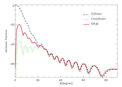
Figure 3: Co–polar, Cross–polar and function $f$ (see text) patterns for the feed horn of the SPOrt experiment at 22 GHz in the $45^{\rm o}$ direction.

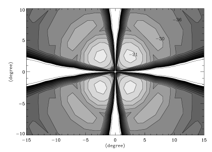
Figure 4: Contour plot of the function $f$ for the 22 GHz feed horn of SPOrt (HPBW $=7^{\rm o}$). Levels are in dB (3 dB by 3 dB) and the maximum level is -21 dB (the 4 main lobes). The function is dominated by a structure with 4 lobes, whose sizes are $\sim 5^{\rm o}$ and whose distances are $\sim 7^{\rm o}$. As a consequence, the anisotropy smoothed on the $\sim$HPBW angular scale is responsible for the instrumental polarisation by the feed horn.

By considering that the anisotropy of the CMB is about 30 $\mu$K on $7^{\rm o}$ angular scale, the contribution of the feed horn can be considered negligible. In fact, in the case of the example of the Figure 4, the integral value of the function $f(\theta,\,\phi)$ with respect to the integral of the co–polar pattern $F_{e}(\theta,\,\phi)$ is $\sim-25$ dB, which yields to a correlation term of the order of 0.1 $\mu$K.

4.1.2 Polariser

The polariser can be described by a 4 ports device whose outputs can be expressed in the reference frame defined by its two principal linear polarisations as follows

$$E_{\parallel} = S_{\parallel}\left(V^{F}_{\parallel}+N^{\rm pol}_{\parallel}\right)$$

$$E_{\perp} = S_{\perp}\left(V^{F}_{\perp}+N^{\rm pol}_{\perp}\right)$$ (20)

where $N^{\rm pol}_{\parallel}$ and $N^{\rm pol}_{\perp}$ are the noise generated by the polariser and evaluated at its input. The parameters $S_{\parallel}$ and $S_{\perp}$ are the related transmission parameters. In ideal conditions $S_{\parallel}=1$ and $S_{\perp}=j$ (omitting the common phase delay).

4.1.3 OMT

The OMT can be described as a 4 port network as well. In the OMT reference frame the input signals are:

$$E_{1} = \frac{1}{\sqrt{2}}\left[S_{\parallel}\left(V^{F}_{\parallel}+N^{\rm pol}_{\parallel}\right)-S_{\perp}\left(V^{F}_{\perp}+N^{\rm pol}_{\perp}\right)\right]$$

$$E_{2} = \frac{1}{\sqrt{2}}\left[S_{\parallel}\left(V^{F}_{\parallel}+N^{\rm pol}_{\parallel}\right)+S_{\perp}\left(V^{F}_{\perp}+N^{\rm pol}_{\perp}\right)\right]$$ (21)

and the output signals can be written as a linear combination of the input ones:

$$A = S_{A1}(E_{1}+N^{\rm OMT}_{1})+S_{A2}(E_{2}+N^{\rm OMT}_{2})$$

$$B = S_{B1}(E_{1}+N^{\rm OMT}_{1})+S_{B2}(E_{2}+N^{\rm OMT}_{2})$$ (22)

where $S_{A1}$, $S_{A2}$, $S_{B1}$, $S_{B2}$ are the OMT transmission parameters, that in ideal conditions must be $S_{A1}/S_{B2}=1$, $|S_{A1}|=1$, and $S_{A2}=S_{B1}=0$. $N_{1}^{\rm OMT}$ and $N_{2}^{\rm OMT}$ denote the noise generated in the two OMT arms and carried to the OMT input.

From equations 21 and 22, $A$ and $B$ become

$$A = \frac{1}{\sqrt{2}}\left[\right.\left(S_{A1}+S_{A2}\right)S_{\parallel}\left(N^{\rm pol}_{\parallel}+V^{F}_{\parallel}\right)-\left(S_{A1}-S_{A2}\right)S_{\perp}\left(N^{\rm pol}_{\perp}+V^{F}_{\perp}\right)\left.\right]$$

$$+S_{A1}N_{1}^{\rm OMT}+S_{A2}N_{2}^{\rm OMT}$$

$$B = \frac{1}{\sqrt{2}}\left[\right.\left(S_{B1}+S_{B2}\right)S_{\parallel}\left(N^{\rm pol}_{\parallel}+V^{F}_{\parallel}\right)-\left(S_{B1}-S_{B2}\right)S_{\perp}\left(N^{\rm pol}_{\perp}+V^{F}_{\perp}\right)\left.\right]$$ (23)

$$+S_{B1}N_{1}^{\rm OMT}+S_{B2}N_{2}^{\rm OMT}$$

4.1.4 Contamination Terms

The spurious polarization can be estimated by computing the product $AB^{*}$, which is the spectral density of the spurious contribution to the measured polarization:

$$AB^{*} = \frac{1}{2}\left(S_{A1}S_{B1}^{*}+S_{A2}S_{B2}^{*}\right)\left[\left|S_{\parallel}\right|^{2}\left(\left|N_{\parallel}^{\rm pol}\right|^{2}+\left|V_{\parallel}^{F}\right|^{2}\right)+\left|S_{\perp}\right|^{2}\left(\left|N_{\perp}^{\rm pol}\right|^{2}+\left|V_{\perp}^{F}\right|^{2}\right)\right]$$ (24)

$$+ \frac{1}{2}\left(S_{A1}S_{B2}^{*}+S_{A2}S_{B1}^{*}\right)\left[\left|S_{\parallel}\right|^{2}\left(\left|N_{\parallel}^{\rm pol}\right|^{2}+\left|V_{\parallel}^{F}\right|^{2}\right)-\left|S_{\perp}\right|^{2}\left(\left|N_{\perp}^{\rm pol}\right|^{2}+\left|V_{\perp}^{F}\right|^{2}\right)\right]$$

$$+ S_{A1}S_{B1}^{*}\left|N_{1}^{\rm OMT}\right|^{2}+S_{A2}S_{B2}^{*}\left|N_{2}^{\rm OMT}\right|^{2}$$

where the antenna signals, the polariser and OMT noises are assumed to be uncorrelated so that their crossed products are zero.

Under matching conditions, for the $\parallel$ channel of the polariser the spectral density of the noise can be written in terms of equivalent antenna temperature

$$\left|N_{\parallel}^{\rm pol}\right|^{2} = \left(\frac{1}{\left|S_{\parallel}\right|^{2}}-1\right)T_{\rm ph}^{\rm pol}\;=\;T_{\rm noise}^{\rm pol}$$ (25)

where $T_{\rm ph}^{\rm pol}$ is the polariser physical temperature and $T_{\rm noise}^{\rm pol}$ is the polariser equivalent noise temperature at its input section. For $N_{\perp}$ a similar expression holds.

Because of the presence of the cross–coupling terms $S_{B1}$ and $S_{A2}$, the noise produced by the OMT cannot be directly derived, as for the polarizer. One should diagonalize the transmission operator, but this would require the knowledge of its scattering matrix and, moreover, the diagonalization should be frequency independent. However, under the assumption that the off-diagonal terms are much smaller than the diagonal ones, a conservative estimation of the OMT noise is:

$$\left|N_{1}^{\rm OMT}\right|^{2} = \left(\frac{1}{\left|S_{A1}\right|^{2}}-1\right)T_{\rm ph}^{\rm OMT}\;=\;T_{\rm noise}^{\rm OMT}$$ (26)

where $T_{\rm ph}^{\rm OMT}$ is the OMT physical temperature and $T_{\rm noise}^{\rm OMT}$is the OMT equivalent noise temperature at its input. For the noise $N_{2}^{\rm OMT}$ a similar formula holds, where $S_{A1}$ is substituted with $S_{B2}$.

Finally, the expression for the antenna signal is

$$\left|V_{\parallel}^{F}\right|^{2} = \eta\,T_{A}$$ (27)

$$= \eta\left[\left(\frac{1}{\eta}-1\right)T_{\rm ph}^{\rm horn}+T_{\rm sky}+T_{\rm atm}\right]$$

$$= \eta\left(T_{\rm noise}^{\rm horn}+T_{\rm sky}+T_{\rm atm}\right)$$

where $\eta$ is the efficiency of the feed horn, $T_{\rm ph}^{\rm horn}$ is the feed horn physical temperature, $T_{\rm noise}^{\rm horn}$ is the feed horn equivalent noise temperature carried to the feed horn input section, $T_{A}$ is the total antenna temperature, $T_{\rm sky}$ and $T_{\rm atm}$ are the sky and the atmosphere signals, respectively.

Now, by substituting this expressions in equation 24, it can be written

$$AB^{*} = \frac{1}{2}\left(S_{A1}S_{B1}^{*}+S_{A2}S_{B2}^{*}\right)$$ (28)

$$\left[\left|S_{\parallel}\right|^{2}\left({1\over\left|S_{\parallel}\right|^{2}}-1\right)T_{\rm ph}^{\rm pol}+\left|S_{\perp}\right|^{2}\left({1\over\left|S_{\perp}\right|^{2}}-1\right)T_{\rm ph}^{\rm pol}+\left(\left|S_{\parallel}\right|^{2}+\left|S_{\perp}\right|^{2}\right)\eta\,T_{A}\right]$$

$$+ S_{A1}S_{B1}^{*}\left(\frac{1}{\left|S_{A1}\right|^{2}}-1\right)T_{\rm ph}^{\rm OMT}+S_{A2}S_{B2}^{*}\left(\frac{1}{\left|S_{B2}\right|^{2}}-1\right)T_{\rm ph}^{\rm OMT}$$

$$+ {1\over 2}\left(S_{A1}S_{B2}^{*}+S_{A2}S_{B1}^{*}\right)\left(\left|S_{\parallel}\right|^{2}-\left|S_{\perp}\right|^{2}\right)\left(\eta\,T_{A}-T_{\rm ph}^{\rm pol}\right)$$

In order to evaluate the level of the correlation product $AB^{*}$ it can be assumed that $S_{A1}\sim S_{B2}$, $S_{A2}\sim S_{B1}<<1$ and $|S_{\parallel}|\sim|S_{\perp}|$ where they are summed. In this way, the equation 28 becomes

$$AB^{*} = 2\,\Re(S_{A1}S_{B1}^{*})\left[\left|S_{\parallel}\right|^{2}\left(\frac{1}{\left|S_{\parallel}\right|^{2}}-1\right)T_{\rm ph}^{\rm pol}+\eta\left|S_{\parallel}\right|^{2}T_{A}+\left(\frac{1}{\left|S_{A1}\right|^{2}}-1\right)T_{\rm ph}^{\rm OMT}\right]+$$ (29)

$${1\over 2}\left|S_{A1}\right|^{2}\left(\left|S_{\parallel}\right|^{2}-\left|S_{\perp}\right|^{2}\right)\left(\eta\,T_{A}-T_{\rm ph}^{\rm pol}\right)$$

From equation 29 one can observe that the spurious polarisation of a real antenna system is composed by two terms. The first one is due to the OMT, in fact this term is proportional to the OMT cross–coupling parameter $S_{B1}$, describing the insulation between the two OMT channels. The second term is due to the polariser, because is proportional to $\left|S_{\perp}\right|^{2}-\left|S_{\parallel}\right|^{2}$. It has to be noted that in this term $T_{A}$ and $T_{\rm ph}^{\rm pol}$ have opposite sign.

Finally, this result can be carried to the feed horn input section as follows:

$${AB^{*}}_{0} = {1\over\eta}{1\over\left|S_{\parallel}\right|^{2}}{1\over\left|S_{A1}\right|^{2}}AB^{*},$$ (30)

that through equations 25–27 and 29 transforms in

$${AB^{*}}_{0} = 2\,{\Re(S_{A1}S_{B1}^{*})\over\left|S_{A1}\right|^{2}}\left(T_{\rm sky}+T_{\rm atm}+T_{\rm noise}^{\rm Ant}\right)+$$ (31)

$${1\over 2}\left(1-{\left|S_{\perp}\right|^{2}\over\left|S_{\parallel}\right|^{2}}\right)\left(T_{\rm sky}+T_{\rm atm}+T_{\rm noise}^{\rm horn}-{T_{\rm ph}^{\rm pol}\over\eta}\right),$$

where

$$T_{\rm noise}^{\rm Ant}=T_{\rm noise}^{\rm horn}+{1\over\eta}T_{\rm noise}^{\rm pol}+{1\over\eta}{1\over|S_{\parallel}|^{2}}T_{\rm noise}^{\rm OMT}$$ (32)

is the noise temperature of the whole antenna system. The equation 31 provides a physical insight into the generation of the spurious polarisation and can be directly compared with the polarised radiation level. One can see how the various noise temperatures as well as the sky and atmosphere emission are partially detected as correlated signals because of the OMT cross–talk and the polariser attenuation difference. In particular we can define two quantities that describe the goodness of the OMT and of the polariser from the spurious polarisation point of view:

$$S\!P_{\rm OMT} = 2\,{\Re(S_{A1}S_{B1}^{*})\over\left|S_{A1}\right|^{2}}$$ (33)

$$S\!P_{\rm pol} = {1\over 2}\left(1-{\left|S_{\perp}\right|^{2}\over\left|S_{\parallel}\right|^{2}}\right)$$ (34)

so that the spurious polarisation produced by the OMT and the polariser and evaluated at the input of the antenna can be expressed as

$${AB^{*}}_{0}=S\!P_{\rm OMT}\left(T_{\rm sky}+T_{\rm atm}+T_{\rm noise}^{\rm Ant}\right)+S\!P_{\rm pol}\left(T_{\rm sky}+T_{\rm atm}+T_{\rm noise}^{\rm horn}-{T_{\rm ph}^{\rm pol}\over\eta}\right),$$ (35)

Moreover, following the IAU definition of the polarised brightness temperature $T_{b}^{p}$ (Berkhuijsen 1975), the output for a sky signal, in equivalent antenna temperature at the feed horn input section, is

$${AB^{*}}_{0} = T_{b}^{p}(\cos(2\alpha)+j\sin(2\alpha))$$ (36)

where $\alpha$ is the polarisation angle. Therefore, equation 35 provides the estimate of the spurious polarisation level, which can be directly compared to the polarised brightness temperature.

Since the spurious polarisation represents a polarimeter offset, the value computed in equation 35 is the $T_{\rm offset}$ term of equation 1

4.2 Correlation of Linearly Polarised Components

The case of a polarimeter correlating linearly polarised components ($E_{X}$ and $E_{Y}$) can be faced in a similar way, but in this case the term due to the polariser does not exist. Also in this case the feed horn contribution is negligible, and the spurious polarisation is described by

$$AB^{*} = S_{A1}S_{B1}^{*}\left[\left(\frac{1}{\left|S_{A1}\right|^{2}}-1\right)T_{\rm ph}^{\rm OMT}+\eta\,T_{A}\right]$$ (37)

$$+ S_{A2}S_{B2}^{*}\left[\left(\frac{1}{\left|S_{B2}\right|^{2}}-1\right)T_{\rm ph}^{\rm OMT}+\eta\,T_{A}\right]$$

Following the assumptions adopted for the circular polarisation case, it can be reduced to

$$AB^{*} = 2\,\Re(S_{A1}S_{B1}^{*})\left[\eta\,T_{A}+\left(\frac{1}{\left|S_{A1}\right|^{2}}-1\right)T_{\rm ph}^{\rm OMT}\right].$$ (38)

that at the feed horn input section yields

$${AB^{*}}_{0} = 2\,{\Re(S_{A1}S_{B1}^{*})\over\left|S_{A1}\right|^{2}}\left(T_{\rm sky}+T_{\rm atm}+T_{\rm noise}^{\rm Ant}\right)$$ (39)

$$= S\!P_{\rm OMT}\left(T_{\rm sky}+T_{\rm atm}+T_{\rm noise}^{\rm Ant}\right)$$

Obviously, here the spurious polarisation is due to the OMT cross–talk only.

5 Sensitivity Degradation

The radiometer sensitivity equation (eq. 1) contains the three terms contributing to the rms error in radio measurements. It is clear that both the gain and the offset fluctuation may contribute significantly to the sensitivity degradation, so it is important to estimate the time scale on which their effects are greater than the white noise.

5.1 Gain Fluctuations

The noise density power spectrum of the radiometer output (Wollack & Pospieszalski 1998) provides the way to compare these effects:

$$P(f) = 2{k^{2}\,T_{\rm sys}^{2}\over\Delta\nu}+T_{\rm offset}^{2}\,\delta g^{2}(f)+\delta T_{\rm offset}^{2}(f)$$ (40)

$$= P_{\rm wn}(f)\;\,+P_{\rm g}(f)\;\;\;\;\;\;\;\;\;\;+P_{\rm offset}(f)$$

being $\delta g^{2}(f)$ and $\delta T_{\rm offset}^{2}(f)$ the power spectra of gain and offset fluctuations, respectively.

The first term is the white noise (WN): its power spectrum is constant and it depends only on the istantaneous sensitivity $\sigma_{0}$

$$P_{\rm wn}(f)=2\,\sigma_{0}^{2}=2\,{k^{2}T_{\rm sys}^{2}\over\Delta\nu}.$$ (41)

The second term represents the contribution of (amplifier chain) gain fluctuations to the noise power spectrum and it depends on $T_{\rm offset}$. This makes a correlator more stable than a direct detection receiver, for which $T_{\rm sys}$ must be considered instead of $T_{\rm offset}$. Then, in a correlator receiver the contribution of gain fluctuations is a factor $(T_{\rm offset}/T_{\rm sys})^{2}$ lower than in a direct detection receiver.

Since $\delta g^{2}\propto f^{-\beta}$ (Wollack, 1995; Wollack & Pospieszalski, 1998) the second term of equation 40 can be written as

$$P_{\rm g}(f)=2\,\sigma_{0}^{2}\left({f_{k}\over f}\right)^{\beta}$$ (42)

where the knee frequency $f_{k}$ is the frequency at which the gain fluctuation noise equals the white noise ($\beta$ tipically is $\sim 1$), that is the knee frequency defines the time scale at which gain fluctuations become higher than the instrument white noise. Since a correlation receiver is more stable by a factor $(T_{\rm offset}/T_{\rm sys})^{2}$, the relationship between the knee frequencies of a direct detection ($f_{k}$) and a correlation ($f_{k}^{c}$) receiver based on the same amplifier chain is

$$f_{k}^{c}=\left(T_{\rm offset}\over T_{\rm sys}\right)^{2/\beta}\!\!\!\!\!f_{k}\;\;\simeq\;\;\left(T_{\rm offset}\over T_{\rm sys}\right)^{2}f_{k}$$ (43)

Note that $f_{k}^{c}$ scales as $\sim(T_{\rm offset}/T_{\rm sys})^{2}$ so that, for instance, a ratio $T_{\rm offset}/T_{\rm sys}=10^{-2}$ makes the correlator stable on a time scale $10^{4}$ longer than an equivalent direct detection receiver.

Table 1 shows offset estimates, computed through equations 35 and 39, for 5 types of experiment. L&R@30 and L&R@90 are ground based polarimeters correlating the left–hand and right–hand circular components at 30 and 90 GHz, respectively, whereas X&Y@30 and X&Y@90 are the cases for linear components. For all of them attenuations have been assumed to be $1/\eta=0.05$ dB, $1/|S_{C}|^{2}=0.2$ dB, $1/|S_{A1}|^{2}=0.2$ dB for feed horn, polariser and OMT, respectively, together with a common physical temperature of 20K. Moreover, as typical values for CMB experiments are assumed: OMT insulation $|S_{B1}|^{2}\sim-30$ dB and polariser spurious term $|S_{L}|^{2}-|S_{C}|^{2}\sim-30$ dB. Finally, it has been considered also the SPOrt case, the only scheduled space experiment designed to measure the microwave sky polarisation, where physical temperatures are: $T_{\rm ph}^{\rm horn}\sim 300{\rm K}$ and $T_{\rm ph}^{\rm pol}=T_{\rm ph}^{\rm OMT}\sim 80{\rm K}$; attenuations has been assumed as for other experiments. However, since high care has been taken developing the OMT, its insulation term is $|S_{B1}|^{2}\leq-60$ dB; again, conservatively, $|S_{L}|^{2}-|S_{C}|^{2}\sim-30$ dB is assumed. Also without atmospheric contributions, the OMT is again the main offset source through the cross–correlation of the antenna noise.

Table 1: Offset estimates for 4 typical ground experiments at 30 and 90 GHz (see text) and for the SPOrt experiment. Different offset contributions due to the OMT (upper part) and to the polariser (bottom part) are expressed in mK. Atmospheric contributions are calculated for typical values at Antarctica sites: $T_{\rm atm}(30{\rm GHz})\sim 7{\rm K}$ and $T_{\rm atm}(90{\rm GHz})\sim 10{\rm K}$ (Bersanelli et al. 1995, Danese & Partridge 1989).

	L&R@30	X&Y@30	L&R@90	X&Y@90	SPOrt
$S\!P_{\rm OMT}T_{\rm noise}^{\rm horn}$	$15$	$15$	$15$	$15$	$7$
$S\!P_{\rm OMT}T_{\rm noise}^{\rm pol}$	$60$	-	$60$	-	$8$
$S\!P_{\rm OMT}T_{\rm noise}^{\rm OMT}$	$63$	$60$	$63$	$60$	$8$
$S\!P_{\rm OMT}T_{\rm sky}$	$170$	$170$	$170$	$170$	$5$
$S\!P_{\rm OMT}T_{\rm atm}$	$442$	$442$	$632$	$632$	$0$
Total OMT	$750$	$687$	$940$	$877$	$28$
$S\!P_{\rm pol}T_{\rm noise}^{\rm horn}$	$\sim 0$	-	$\sim 0$	-	$\sim 2$
$S\!P_{\rm pol}T_{\rm ph}^{\rm pol}/\eta$	$10$	-	$10$	-	$39$
$S\!P_{\rm pol}T_{\rm atm}$	$3.5$	-	$5.0$	-
$S\!P_{\rm pol}T_{\rm sky}$	$\sim 1$	-	$\sim 1$	-	$\sim 1$
Total Polariser	$14.5$	-	$16$	-	$42$
Total (OMT+Polariser)	$764$	$687$	$956$	$877$	$70$

Table 1 data suggest that ground based experiments have offsets mainly due to atmosphere emission rather than to the sky signal. Moreover, since this offset is due to the cross–correlation of the OMT, correlating either the circularly or the linearly polarised component is quite equivalent from the offset generation point of view.

Table 2: Knee frequencies for the 5 experiments of Table 1 calculated through equation 43. The maximum allowed modulation time $t_{m}$ is also reported. $T_{\rm sys}$ and $f_{k}$ evaluations for ground experiments are based on the best available HEMT (NRAO) and were taken from Keating et al. 1998, Wollack & Pospieszalki 1998. The SPOrt parameters have been calculated for TRW–MMIC amplifiers (Gaier et al. 1996; see also Cortiglioni et al. 1999).

	L&R@30	X&Y@30	L&R@90	X&Y@90	SPOrt
$T_{\rm sys}$ (K)	$30$	$30$	$80$	$80$	$150$
$T_{\rm offset}$ (mK)	$764$	$687$	$956$	$877$	$70$
$f_{k}$ (Hz)	$50$	$50$	$2\times 10^{3}$	$2\times 10^{3}$	$50$
$f_{k}^{c}$ (Hz)	$3.2\times 10^{-2}$	$2.6\times 10^{-2}$	$2.9\times 10^{-1}$	$2.4\times 10^{-1}$	$1.1\times 10^{-5}$
$t_{m}$ (s)	$31$	$38$	$3.5$	$4.2$	$9.2\times 10^{4}$

Table 2 reports the knee frequencies for the five experiments taken as example, computed by using the offset values of Table 1. The knee frequency allows the estimate of the time

$$t_{m}\sim{1\over f_{k}^{c}}$$ (44)

after that long term drifts degradate the radiometer sensitivity. Signal modulation techniques help to overcome this degradation, but the modulation frequency must be greater than $f_{k}^{c}$. Table 2 shows, for example, that ground based experiments would need modulation time $\leq 40$ s (30 GHz experiments) or $\leq 4$ s (90 GHz experiments). SPOrt looks much more stable and its $t_{m}$ parameters exceeds largely its modulation time (5400s i.e. its orbital period, see Cortiglioni et al. 1999). It should be noted that such a modulation must be inserted before the components responsible of the offset generation, to be effective.

5.2 Offset Fluctuations

The offset fluctuation is the second sensitivity degradation term of equation 1. Equations 35 and 39 show that it depends on both the physical temperature and atmospheric emission fluctuations (only for ground based experiment).

Monitoring of physical temperatures and cross–correlations with the data may allow the reduction of this contribution during off-line analysis, but atmospheric fluctuations cannot be recovered and their power spectrum adds to the white noise one. In principle, the atmospheric emission is unpolarised, but the spurious polarisation generated by OMT losses fluctuates as the atmospheric emission does. As in the case of gain fluctuations, the impact on the sensitivity can be estimated in terms of noise power spectrum.

Atmospheric offset fluctuations can be written, following equation 35, as

$$\Delta T_{\rm offset} = (S\!P_{\rm OMT}+S\!P_{\rm pol})\,\Delta T_{\rm atm}$$ (45)

$$= S\,\Delta T_{\rm atm}$$

and their contribution to the noise power spectrum is given by

$$P_{\rm offset} = S^{2}P_{\rm atm}$$ (46)

which adds to the white noise and gain fluctuations power spectra, being them uncorrelated.

Measurements taken at sea level site (Smoot et al., 1987) show that at 90 GHz the atmospheric fluctuations follow a power law

$$P_{\rm atm}(f)=\propto\,f^{-\alpha}\>\>\>\>{\rm for}\;f\in[10^{-3},10^{-1}[$$ (47)

with $\alpha=8/3$ and normalisation $P_{\rm atm}(0.02{\rm Hz})\sim 1{\rm K^{2}\,Hz^{-1}}$. Under these assumptions,

Table 3: Power spectrum values of both the 90 GHz atmospheric emission and offset fluctuations at several frequencies $f$ obtained from equations 46 and 47, assuming the normalisation $P_{\rm atm}(0.02{\rm Hz})\sim 1{\rm K^{2}\,Hz^{-1}}$. The coefficient $S$ has been computed from antenna parameters as in Table 1.

$f$ (Hz)	$P_{\rm atm}$ (mK2Hz-1)	$P_{\rm offset}$ (mK2Hz-1)
$0.02$	$1.0\times 10^{6}$	$4.3\times 10^{3}$
$0.03$	$3.4\times 10^{5}$	$1.4\times 10^{3}$
$0.1$	$1.4\times 10^{4}$	$5.5\times 10^{1}$
$0.3$	$7.3\times 10^{2}$	$3.0$
$1$	$2.9\times 10^{1}$	$0.12$

Table 3 shows typical power spectrum values for both the atmosphere emission and the corresponding polarimeter offset at different frequencies. Similarly to the gain, offset fluctuations begin to degradate the ideal (white noise) sensitivity when $P_{\rm offset}>P_{\rm wn}$. Since 90 GHz radiometer amplifiers (HEMT) have typically $P_{\rm wn}=0.64$ mK²Hz^-1 (see Wollack & Pospieszalski 1998), the offset fluctuations get over the white noise level at $f<0.5$ Hz (see Figure 5). Consequently, modulation techniques with modulation time $t_{m}<2$ s are required for longer integration time.

Figure 5: Estimate of the power spectrum of the offset fluctuations induced by atmospheric fluctuations for a 90 GHz experiment as from Table 3 (solid line). The white noise power spectrum of a typical 90 GHz amplifier is also shown (dashed, Wollack & Pospieszalski 1998). The two spectra are comparable at $f\sim 0.5$ Hz suggesting a modulation time of $t_{m}\sim 2$ s.

Such a low $t_{m}$ value suggests to estimate the parameter $S$ and the insulation of the OMT needed to ehhance it, for example, up to $t_{m}=1000$ s or, equivalently, to have $P_{\rm offset}(f=$ $10^{-3}{\rm Hz})=P_{\rm wn}$ ($f=10^{-3}$ Hz represents the limit of equation 47). From equation 47 and Table 3 it can be estimated $P_{\rm atm}(10^{-3})\sim 2.9$ mK²Hz^-1, implying $S^{2}\sim 2.2\times 10^{-10}$, that is an OMT insulation $|S_{B1}|^{2}<-100$ dB (!) and a difference between the two attenuations of the polariser $(|S_{\parallel}|^{2}-|S_{\perp}|^{2})<-45$ dB.

At 30 GHz the water vapour emission and its fluctuations (the main responsible for atmospheric fluctuations) are 6 times lower than at 90 GHz. The corresponding $P_{\rm offset}$ is 36 times lower, bringing to a slightly better situation. In fact, using Table 3 a suitable modulation time $t_{m}<8$ s can be estimated.

In principle, the best sites (like Antarctica), where expected atmospheric fluctuations are lower, allow higher $t_{m}$, that become comparable with values called by gain fluctuations (see Table 2).

6 Conclusions

The main aim of this paper is to analyse carefully the problem related to the instrumental (spurious) polarisation, that is generated inside the instrument itself, because it can represent the major source of sensitivity degradation. The reason for this is that also unpolarised signal components, genuinely uncorrelated, would become correlated noise due to losses in real receiver components. Such a correlated noise contributes to produce an offset which is responsible of sensitivity degradation (through gain and offset fluctuations) that, in some cases, can be an insurmountable obstacle to the measure. That is the case, in particular, of the atmosphere emission, which is in principle unpolarised being of thermal origin.

It has been recognised that CMBP investigations require state of the art receivers, able to give system noise, and consequently instantaneous sensitivity, as low as possible. However, it is well known that in any case CMBP measurements should require long integration times because of the extremely low expected signal (10% of the anisotropy or less). As a consequence, the most challenging aspect of such a measurements is the long term stability, which is the base for useful long integration times.

This paper has given some algorithms for spurious polarisation evaluations in different instrumental configurations, identifying the OMT cross–coupling and the polariser attenuation difference as the major causes of correlated noise generation. It has been also demonstrated that the antenna system is responsible of most of the instrumental offset production, which represents the true limit to long integration times needed by CMBP measurements.

The most relevant conclusion is that the best ground based experiment at 30 GHz (90 GHz) cannot ensure integration times longer than 40 s (4 s) without modulation. Alternatively, most critical components like OMT and polariser should have characteristics that are not present at all in commercially available devices. As a consequence a significant step towards detection of CMBP with microwave radiometers should pass through new instrumental configurations based on custom components, rather than on low system noise only. An example of such a philosophy is the SPOrt experiment, that shows how much the long term stability can be improved by using custom designed components together with correlation techniques.

References

- [1] Baccigalupi C., Burigana C., Perrotta F., De Zotti G., La Porta L., Maino D., Maris M., Paladini R., 2000, submitted to A&A (astro–ph/0009432)
- [2] Bennet C.L. et al., 1996, ApJ, 464, L1
- [3] Bennet C.L. et al., 1997, in AAS Meeting 191, #87.01
- [4] Berkhuijsen E.M., 1975, A&A, 40, 311
- [5] Bersanelli M., Bensadoun M., Danese L., de Amici G., Kogut A., Levin S., Limon M., Maino D., Smoot, G.F., Witebsky C., 1995, ApJ, 448, 8
- [6] Bouchet F.R., Prunet S., Sethi S.K., 1999, MNRAS, 302, 663
- [7] Brandt W.N., Lawrence C.R., Readhead A.C.S., Pakianathan J.N., Fiola T.M., 1994, ApJ, 424, 1
- [8] Brouw W.N., Spoelstra T.A.Th., 1976, A&AS, 26, 129
- [9] Carretti E., et al., 2000, in New Cosmological Data and the Values of the Fundamental Parameters, IAU Symposium #201, ASP Conf. Ser., in press
- [10] Carretti E., et al., 2001, in preparation
- [11] Cortiglioni S., 1995, Rev. Sci. Instrum., 65, 2667
- [12] Cortiglioni S. et al., 1999, in 3K Cosmology, AIP Conference Proceedings 476, 186
- [13] Danese L., Partridge R.B., 1989, ApJ, 342, 604
- [14] De Bernardis P. et al., 2000, Nature, 404, 955
- [15] Draine B.T., Lazarian A., 1999, in Microwave Foregrounds, Eds. A. de Oliveira–Costa & M. Tegmark, ASP Conf. Ser., 181, 133
- [16] Dodelson S., 1997, ApJ, 482, 577
- [17] Duncan A.R., Haynes R.F., Jones K.L., Stewart R.T., 1997, MNRAS, 291, 279
- [18] Duncan A.R., Reich P., Reich W., Fürst, E., 1999, A&A, 350, 447
- [19] Efstathiou G., Bond J.R., 1999, MNRAS, 304, 75
- [20] Fixsen D.J., Cheng E.S., Gales J.M., Mather J.C., Shafer R.A., Wright E.L., 1996, ApJ, 473, 576
- [21] Gaensler B., Dickey J., McClure–Griffiths N., Green A., Wieringa M., Haynes R., 2001, ApJ, in press (astro-ph/0010518)
- [22] Gaier T. et al. 1996, in Millimeter and Submillimeter Waves and Applications III, ed. M.N. Afsar, Proc. SPIE, 2842, 46
- [23] Hanany S. et al., 2000, ApJ, 545, L5
- [24] Hedman M.M., Barkats D., Gundersen J.O., Staggs S.T., Winstein B., 2000, ApJL, in press (astro-ph/0010592)
- [25] Jungman G., Kamionkowski M., Kosowsky A., Spergel D.N., 1996, PRD, 54, 1332
- [26] Junkes N., Fürst E., Reich W., 1987, A&AS, 69, 451
- [27] Kamionkowski M., Kosowsky A., 1998, PRD, 57, 685
- [28] Keating B., Timbie P., Polnarev A., Steinberger J., 1998, ApJ, 495, 580
- [29] Kogut et al., 1996, ApJ, 470, 653
- [30] Kogut A., Hinshaw G., 2000, ApJ, 543, 530
- [31] Kraus J.D., 1986, Radio Astronomy, (Ed. Cygnus–Quasar Books: Powell, OH)
- [32] Lazarian A., Draine B.T., 2000, 536, L15
- [33] McClure-Griffiths N.M., Green A.J., Dickey J.M., Gaensler B.M., Haynes R.F., Wieringa M.H., 2001, ApJ, in press (astro-ph/0012302)
- [34] Miller A.D., Caldwell R., Devlin M.J., Dorwart W.B., Herbig T., Nolta M.R., Page L.A., Puchalla J., Torbet E., Tran H. T., 1999, ApJ, 524, L1
- [35] Prunet S., Sethi S.K., Bouchet F.R., Miville–Deschenes M.-A., 1998, A&A 339, 187
- [36] Revenu B., Kim A., Ansari R., Couchot F., Delabrouille J., Kaplan J., 2000, A&AS, 142, 499
- [37] Rohlfs K., Wilson T.L., 2000, Tools of Radio Astronomy (Ed. Springer Verlag: Heidelberg, Germany)
- [38] Sironi G., Boella G., Bonelli G., Brunetti L., Cavaliere F., Gervasi M., Giardino G., Passerini A., 1997, NewA, 3, 1
- [39] Smoot G.F., 1999, in Microwave Foregrounds, Eds. A. de Oliveira–Costa & M. Tegmark, ASP Conf. Ser., 181, 61
- [40] Smoot G.F. et al., 1991, ApJ, 396, L1
- [41] Smoot G.F., Levin S., Kogut A., De Amici G., Witebsky C., 1987, Radio Sci., 4, 421
- [42] Staggs S.T., Gundersen J.O., Church S.E., 1999, in Microwave Foregrounds, ed. A. de Oliveira-Costa & M. Tegmark, ASP Conference Series, 181, 299
- [43] Tauber J.A., 2000, in New Cosmological Data and the Values of the Fundamental Parameters, IAU Symposium #201, ASP Conf. Ser., in press
- [44] Tegmark M., Eisenstein D.J., Hu W., de Oliveira–Costa A., 2000, ApJ, 530, 133
- [45] Tucci M., Carretti E., Cecchini S., Fabbri R., Orsini M., Pierpaoli E., 2000a, NewA, 5, 181
- [46] Tucci M. et al., 2000b, in New Cosmological Data and the Values of the Fundamental Parameters, IAU Symposium #201, ASP Conf. Ser., in press
- [47] Uyaniker B., Fürst E.; Reich W., Reich P., Wielebinski R., 1999, A&AS, 138, 31
- [48] Wollack E.J., 1995, Rev. Sci. Instrum., 66, 4305
- [49] Wollack E.J., Pospieszalski M.W., 1998, IEEE MTT-S Digest, p. 669
- [50] Wright E.L., 1999, NewAR, 43, 257
- [51] Zaldarriaga M., Spergel D.N., Seljak U., 1997, ApJ, 488, 1