Codes for optically thick and hot photoionized media - Radiative transfer and new developments

Abstract

We describe a code designed for hot media (T $\geq$ a few 10⁴ K), optically thick to Compton scattering. It computes the structure of a plane-parallel slab of gas in thermal and ionization equilibrium, illuminated on one side or on both sides by a given spectrum. This code has been presented in a previous paper (Dumont, Abrassart & Collin 2000), where several aspects were already discussed. So we focus here mainly on the recent developments. Presently the code solves the transfer of the continuum with the Accelerated Lambda Iteration method (ALI) and that of the lines in a two stream Eddington approximation, without using the local escape probability formalism to approximate the line transfer. This transfer code is coupled with a Monte Carlo code which allows to take into account direct and inverse Compton diffusions, and to compute the spectrum emitted up to MeV energies, in any geometry. The influence of a few physical parameters is shown, and the importance of the density and pressure distribution (constant density, pressure equilibrium, or hydrostatic equilibrium) is stressed. Recent improvements in the treatment of the atomic data are described, and foreseen developments are mentioned.

Observatoire de Paris, Section de Meudon, Place Janssen, F-92195 Meudon, France

1. Introduction

The average continuum observed in Active Galactic Nuclei (AGN) is shown in Fig. 1 from the optical to X-ray range, as obtained from a composite optical-UV spectrum of Francis et al. (1991) and Zheng et al. (1997), and from an average (slightly modified) soft X-ray spectrum of Laor et al. (1997). It is widely admitted since several years that the optical-UV part of this continuum is produced by a warm (temperature of the order of $10^{5}\ -\ 10^{6}$ K), optically thick or effectively thick medium, most likely an accretion disc. Moreover, one deduces from the spectral distribution in the hard X-ray range, in particular the 30 keV hump observed in many Seyfert 1 galaxies, and from the presence of other features like the iron K line around 7 keV, that this medium is irradiated by a hard X-ray source, which is partly reprocessed and reemitted (improperly named “reflected”). So one sees a combination of the primary and of the reflected spectra (Ross & Fabian 1993, and many subsequent works). In another interpretation the UV-X continuum is produced by clouds from a disrupted disk (Collin-Souffrin et al. 1996, Czerny & Dumont 1998), and in this case one would also see the spectrum emitted by the non illuminated surface of the clouds. In both interpretations the UV-soft X spectrum is emitted by a dense and thick shell (density higher than 10¹² cm^-3, Thomson thickness higher than unity), irradiated by an X-ray continuum. Similar conditions are met in X-ray binary stars.

Figure 1.: Average continuum of radio loud and radio quiet Active Galactic Nuclei, in arbitrary units.

It is necessary to compute the structure of such an irradiated medium to predict the observed spectrum. Therefore one has to build “intermediate”codes, between those designed for planetary nebulae or Narrow or Broad Line Regions in AGN, and those designed for stellar atmospheres. These codes have to be valid for thick or semi-infinite dense media, eventually hot, irradiated by a non thermal continuum extending in the hard X-rays, to cover the whole range of situations encompassed in AGN and in binary stars.

Owing to the high optical thickness of the medium in several frequency ranges, such codes require that the transfer of both the continuum and the lines be solved in an “exact” way, that is avoiding approximations such as local escape approximation (for the lines) or one stream approximation (for the continuum). Since the medium is generally dense and sometimes close to Local Thermodynamical Equilibrium (LTE), they require that all processes and inverse processes be carefully handled. Being irradiated by an X-ray continuum, the medium contains a large number of ionic species, from low to high ionization, which should all be introduced in the computation. Finally, the medium being hot and thick, not only Thomson, but also Compton scattering, should be taken into account.

We have undertaken to build a code which satisfies these requirements, to compute the emission spectrum produced by irradiated thick and hot media like those commonly assumed in AGN close to the black hole, in a wide range of photon energy. Precisely we have built several interconnected codes, which allow more flexibility. The ensemble is far from being perfect and still contains several approximations which restrict its use, but we improve it gradually.

TITAN is designed to study the structure of a warm or hot thick photoionized gas, and to compute its emission - reflection - transmission spectrum from the infrared up to about 20 keV. It solves the energy balance, the ionization and the statistical equilibria, the transfer equations, in a plane-parallel geometry, for the lines and the continuum. Then, given the thermal and ionization stratification, the computation of the emitted spectrum from 1 keV to a few hundreds keV is performed with NOAR which uses a Monte-Carlo method taking into account direct and inverse Compton scattering (it allows also to study various geometries). In a previous paper (Dumont, Abrassart & Collin 2000) TITAN and its interconnection with NOAR were described. We recall here the main characteristics of the code, and we describe recent improvements as well as new results, focussing only on the aspects which are not treated in a standard way.

We briefly summarize below the physical processes (Section 2), the transfer method and the iteration procedure (Section 3). The influence of the physical parameters, of the atomic data, and of the density distribution, are discussed in Section 4. The coupling of TITAN and NOAR is briefly described in Section 5.

2. Generalities about TITAN

2.1. Physical processes

In TITAN, the physical state of the gas (temperature, ionic abundances and level populations of all ionic species), is computed at each depth, assuming stationary state, i.e.: local balance between ionizations and recombinations, local balance between excitations and deexcitations, local energy balance, and finally total energy balance (equality between inward and outward fluxes).

The ionization equilibrium equations include radiative ionizations by continuum and line photons, collisional ionizations and recombinations, radiative and dielectronic recombinations, charge transfer by H and He atoms, the Auger effects, and ionizations by high energy electrons arising from ionizations by X-ray photons. The emission-absorption mechanisms of the continuum include free-free and free-bound processes, two-photon process, and Thomson electron scattering. Inverse processes (except autoionization for dielectronic recombinations, and recombinations onto excited levels for some ions, see next section) are computed through the equations of detailed balance. Induced processes are taken into account. Energy balance equations include the same processes and Compton heating/cooling.

2.2. Atomic data

Hydrogen and hydrogen-like ions are treated as 5 or 6-level atoms. In a first step, in order to save computation time, non hydrogen-like ions were treated with a rough approximation: interlocking between excited levels was neglected and the populations of excited levels were computed separately using a two-level approximation. This approximation does not predict correctly the details of the line spectrum, including the resonance lines themselves. Moreover ionizations from excited levels were not taken into account, though recombinations onto excited states were taken into account in the ionization equilibrium. This approach is is not correct close to LTE, and even far from LTE, if ones wants to predict accurately detailed spectral features (cf. Section 4.2). However it gives a correct overall spectral distribution in this last case. Such are the upper layers of an irradiated atmosphere where at the same time the fractional abundances of heavy elements in high ionization states are important, and the ground level of these ions is strongly overpopulated with respect to LTE. But it is not the case in the deep layers of a disk atmosphere, emitting the UV part of the spectrum, where the density is high, and the influence of the external irradiation is small.

This is why helium-like ions treated as complete 8-level atoms and lithium-like ions treated as complete 5-level atoms have been recently implemented in the code. All processes are thus taken into account for each level. This treatment is valid as far as the upper levels are in LTE with the continuum. To handle intermediate cases, we replace the missing upper levels which are very important especially for helium-like ions by adding an additional recombination rate, not compensated by ionization.

In the future we plane to add several other levels, and to sum the contributions of the higher levels to handle at the same time cases close to and cases far from LTE.

Photoionization cross sections are fitted from Topbase (cf. Cunto et al 1993). Cross sections of neutral and once ionized heavy elements are not well represented, but they do not have any influence on these hot media.

The gas composition include 10 elements (H, He, C, N, O, Ne, Mg, Si, S, Fe), and all their ionic species.

The slab is divided in about 300 layers with variable thicknesses. The code can work with a prescription for the density or for the pressure, such as a constant pressure or a pressure corresponding to hydrostatic equilibrium.

2.3. Illumination

The external illumination can be characterized by an “ionization parameter”, which we choose here as $\xi={4\pi F_{\rm inc}/n_{\rm H}}$, $F_{\rm inc}$ being the frequency integrated flux incident on one side of the slab and $n_{\rm H}$ the hydrogen number density at this surface. Note that there are several other definitions of the ionization parameter, for instance $U$, or $\Xi$, but they correspond basically to the same concept, namely a parameter which determines the ionization state. It is possible to take also into account a flux incident on the back side of the slab.

Presently we mimic a semi-isotropic illumination, but with the ALI transfer method which is implemented (cf. below) it will be possible to take into account the angular distribution of the incident radiation.

3. Radiation transfer

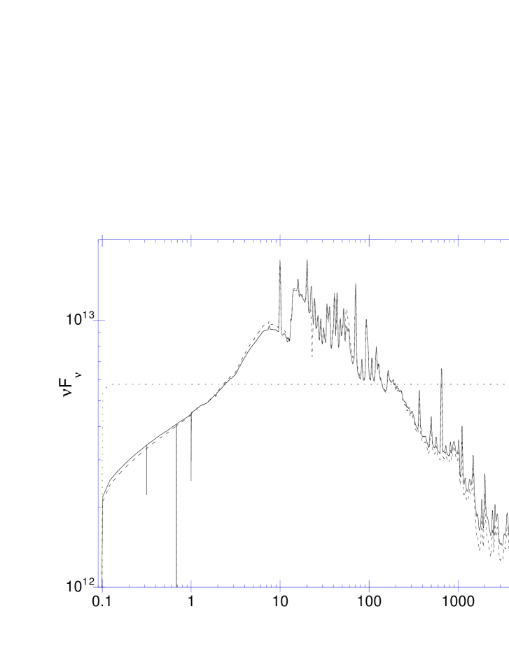
Figure 2.: Reflected spectrum, with (full line), and without (dashed lines) ALI transfer for the continuum, for the reference model defined in Section 4; dotted line: incident spectrum; the spectrum is displayed with a spectral resolution of 30.

We are concerned by media with a continuum optical thickness larger than unity in a range of frequencies rich in emission or in absorption lines, and having a very inhomogeneous structure. Moreover in the hot photoionized layers, the absorption coefficient is weak at all wavelengths and Thomson diffusion is dominant. On the contrary absorption dominates and must be carefully treated to compute the spectrum emitted by the non illuminated cold part of the medium. Radiation transfer requires therefore some attention.

The transfer equation is

$$\mu{dI\over dz}=-(\kappa+\sigma)I+\sigma J+\eta,$$ (1)

where $z$ is the distance to the illuminated surface, $\mu$ is the cosine of the angle between the normal and the light ray, $\kappa$ is the absorption coefficient (for the continuum it is due to photoionizations and free-free transitions), $\sigma$ is the diffusion coefficient (here Thomson scattering), $\eta$ is the emissivity (due to radiative recombinations and free-free emission), and $J$ is the mean intensity, equal to $\int I_{\nu}d\mu/2$ (all these quantities are local, $I$ depends on the direction and on the frequency $\nu$, and J, $\kappa$ and $\eta$ depend on the frequency).

Introducing the source function $S$ and the optical depth $\tau$, Eq. 1 can be written:

$$\mu{dI\over d{\tau}}=-I+S$$ (2)

with

$$S={{\sigma J+\eta}\over{\sigma+\kappa}},$$ (3)

which can be separated between J-dependent and J-independent components:

$$S=(1-\epsilon)J+\epsilon B.$$ (4)

The formal solution is:

$$J(\tau)={1\over 2}\int d\mu\int S(t)e^{-(t-\tau)/\mu}dt/\mu.$$ (5)

3.1. Transfer of the continuum: the ALI method

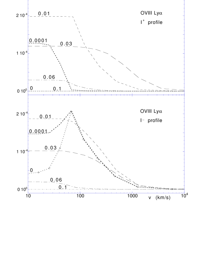
Figure 3.: Profiles of $I_{\nu}^{-}$ and $I_{\nu}^{+}$ for OVIII Ly${\alpha}$, for the reference model defined in Section 4. The curves are labelled by the value of $z/H$.

In the previous version of the code (Dumont et al. 2000) we used the same method for line and continuum transfer, described in Section 3.2. Presently the transfer of the continuum is performed with the Accelerated Lambda Iteration method (ALI), which was set up with the help of subroutines kindly provided to us by F. Paletou (cf. Auer & Paletou 1994, and Kunasz & Auer 1988).

In this method $J(\tau)$ is written with the help of an operator $\bf\large{\Lambda}$:

$$J(\tau)={\bf\large{\Lambda}}[S(t)].$$ (6)

ALI uses an operator splitting, described first by Cannon (1973), then by Olson et al. (1986):

$${\bf\large{\Lambda}}={\bf\large{\Lambda^{*}}}+({\bf\large{\Lambda}}-{\bf\large{\Lambda^{*}}}){\rm\ \ and\ \ }S=S^{*}+\delta S$$ (7)

where $\bf\large{\Lambda^{*}}$ is an approximate $\bf\large{\Lambda}$ operator chosen to facilitate the inversion, and $S^{*}$ has been calculated in the previous iteration. One obtains:

$$\delta S=[1-(1-\epsilon){\bf\large{\Lambda^{*}}}]^{-1}[S-S^{*}].$$ (8)

We use here a parabolic interpolation in the evaluation of the integral giving the intensity from the source function, and an acceleration type Ng (in this method, at every fourth iteration a least squares extrapolation is made in order to reduce the residuals, cf. Ng 1974).

To perform this computation, one needs to know the opacities and emissivities at each frequency as functions of $z$, hence the temperature and the populations at each depth, so an iteration procedure is required.

• For each layer, starting from the illuminated side, the ionization and thermal balance equations are solved by iteration; the temperature, the opacity and the emissivity are computed;

• when the back side of the cloud is reached, the transfer is solved with the ALI method, and $J_{\nu}(z)$ is computed;

• the whole calculation is repeated until convergence with the new values of $J_{\nu}(z)$. It is stopped when the energy balance is achieved for the whole slab (i.e. when the flux entering on both sides of the slab is equal to the flux coming out from both sides). This method is almost as slow as the previous one, albeit more secure.

Fig. 2 shows that the difference in the spectrum computed with the previous transfer method and with ALI is very small. It is certainly due to the fact that the continuum optical thickness is never very large (at most 10⁴). This is not the case at the center of intense lines, which are typically 100 times thicker. We are presently implementing ALI for the line transfer and we expect to find more important differences for a few lines like OVIII L$\alpha$ which are not completely converged even after 1000 iterations (cf. Dumont et al. 2000).

3.2. Line transfer

Since ALI is presently not implemented for the line transfer, it is treated like in the previous version with a simple method based on the Eddington two-stream approximation. In this approximation the transfer equations are written:

$${1\over\sqrt{3}}{dI_{\nu}^{+}\over dz} = -(\kappa_{\nu}+{\sigma\over 2})I_{\nu}^{+}+{\sigma\over 2}I_{\nu}^{-}+\epsilon_{\nu}$$ (9)

$${-1\over\sqrt{3}}{dI_{\nu}^{-}\over dz} = -(\kappa_{\nu}+{\sigma\over 2})I_{\nu}^{-}+{\sigma\over 2}I_{\nu}^{+}+\epsilon_{\nu}.$$

The mean intensity $J_{\nu}$ is equal to $(I_{\nu}^{+}+I_{\nu}^{-})/2$, and the flux $F_{\nu}$ defined as usual by $\int I_{\nu}\cos{\theta}\ d\omega$ is equal to $(I_{\nu}^{+}-I_{\nu}^{-})\ 2\pi/\sqrt{3}$. The “reflected” flux is equal to $I_{\nu}^{-}(0)\ 2\pi/\sqrt{3}$, and the outward flux to $I_{\nu}^{+}(H)\ 2\pi/\sqrt{3}$. The optical depth and the total optical depth are defined as:

$$\tau_{\nu}(z)=\int_{0}^{z}\sqrt{3}(\kappa_{\nu}+\sigma)dz^{\prime}\ \ \ {\rm and}\ \ T_{\nu}=\tau_{\nu}(H)$$ (10)

where $H$ is the total thickness of the slab. For $I_{\nu}^{+}(z)$ the formal solution of the transfer equations between $z-\delta z$ and $z$ is:

$$I_{\nu}^{+}(z)=I_{\nu}^{+}(z-\delta z)e^{-\delta\tau_{\nu}}+e^{-\tau_{\nu}}\int_{\tau_{\nu}-\delta\tau_{\nu}}^{\tau_{\nu}}S_{\nu}(t)e^{+t}dt.$$ (11)

We approximate the source function $S_{\nu}(t)$ by a constant in the interval $z,z+dz$. It leads to:

$$I_{\nu}^{+}(z)=I_{\nu}^{+}(z-\delta z)e^{-\delta\tau_{\nu}}+{{1-e^{-\delta\tau_{\nu}}}\over 2}[S_{\nu}(z-\delta z)+S_{\nu}(z)]$$ (12)

and:

$$I_{\nu}^{-}(z)=I_{\nu}^{-}(z+\delta z)e^{-\delta\tau_{\nu}}+{1-e^{-\delta\tau_{\nu}}\over 2}[S_{\nu}(z+\delta z)+S_{\nu}(z)].$$ (13)

We calculate $S_{\nu}(z)$ and the mean intensity $J_{\nu}(z)$ from Eq. 3 and from:

$$J_{\nu}(z) = {I_{\nu}^{+}(z-\delta z)+I_{\nu}^{-}(z+\delta z)\over 2}e^{-\delta\tau_{\nu}}$$

$$+ {(1-e^{-\delta\tau_{\nu}})\over 4}[S_{\nu}(z-\delta z)+2S_{\nu}(z)+S_{\nu}(z+\delta z)],$$

assuming a constant $\delta z$ (actually it is not constant so the formulae are more complicated but do not deserve to be given here).

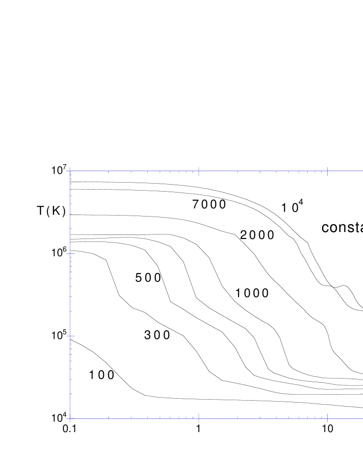
Figure 4.: Temperature versus depth for different values of $\xi$ in erg cm s^-1, the other parameters being the same as in the reference model.

The procedure is then the following:

• for each layer, after computation of the temperature and the source function, $I_{\nu}^{+}(z)$ is transferred through the layer according to Eq. 12, while $S_{\nu}(z)$ and $\tau_{\nu}(z)$ are buffered for each layer and each frequency;

• when the back side of the cloud is reached, new values of $I_{\nu}^{-}(z)$ are calculated, starting from the back side where $I_{\nu}^{-}(H)$ is given by Eq. 12, and using Eq. 13 with the previous values of $S_{\nu}(z)$ and $\tau_{\nu}(z)$ (actually we use the values given by several previous iterations to accelerate the procedure with a Ng method).

This method requires a large number of iterations to get a complete convergence of the model, and one cannot be sure to have reached the correct value. It is why we are now changing for the ALI method.

We assume presently complete redistribution in the lines, and partial redistribution in intense lines is mimicked by assuming complete redistribution in a pure Doppler profile. It will be possible to treat partial redistribution with the ALI method.

A line profile is represented by a Voigt function at several frequencies distributed symmetrically around the line center. The frequencies in the profile are chosen to take into account the fact that the Doppler width may decrease by one order of magnitude inside the slab, owing to large temperature variations. Moreover, to solve the statistical equilibrium equations one needs to know the total line intensity weighted by the profile $\int J_{\nu}\phi(\nu)d\nu$, while to compute the thermal and ionization equilibria one simply needs the line intensity integrated over frequencies $\int J_{\nu}d\nu$. For intense lines, the first integral is dominated by the Doppler core, and the second by the wings. The set of frequencies chosen to describe the line must therefore cover at least two orders of magnitude. The integrals over the line profiles are achieved with a 15-point Gauss-Legendre quadrature. We also assume that the lines do not overlap, which is valid as far as multiplets are treated globally, and because the number of lines taken into account in TITAN is relatively small (presently 580, including subordinate lines in the optical-UV range).

Figure 5.: Reflected and outward spectra for different values of $\xi$ in erg cm s^-1, the other parameters being the same as in the reference model; the spectra are displayed with a spectral resolution of 100.

Figure 6.: Reflected and outward spectra for different values of the column density in cm^-2, for $\xi=100$ erg cm s^-1, the other parameters being the same as in the reference model; the spectra are displayed with a resolution of 100. Dotted line: the incident spectrum.

As shown by Fig. 3, the profiles of $I_{\nu}^{-}$ and $I_{\nu}^{+}$ for OVIII Ly${\alpha}$ vary considerably from the surface to the deepest layers.

4. Some results of TITAN

We shall call “reference model” a model with the following characteristics:

• it is a plan-parallel slab with a constant density, equal to 10¹² cm^-3,

• its column density equals 10²⁶ cm^-2 (corresponding to a Thomson thickness $\tau_{\rm es}$ of 80),

• it is illuminated on one side by an incident power law continuum proportional to $\nu^{-1}$ from 0.1 eV to 100 keV,

• the ionization parameter is $\xi=10^{3}$ erg cm s^-1,

• there is no illumination on the other side,

• the abundances are (in number): H: 1, He: 0.085, C: 3.3 10^-4, N: 9.1 10^-5, O: 6.6 10^-4, Ne: 8.3 10^-5, Mg: 2.6 10^-5, Si: 3.3 10^-5, S: 1.6 10^-5, Fe: 3.2 10^-5.

In several examples given below, we also use a smaller value of the ionization parameter, $\xi=10^{2}$ (corresponding to a value of the usual ionization parameter $U$ equal to 0.88), allowing an easier comparison with computations made with CLOUDY or with XSTAR.

Figs. 4 and 5 show the results corresponding to different values of the ionization parameter, the other parameters being the same as in the reference model. These results were obtained with the previous version of the code. Indeed each model takes a long time to run, and all models have still not been recalculated with the ALI method. However, we have checked in several cases that the results obtained with the new version differ very slightly from the previous ones.

Fig. 4 displays the temperature versus the depth. Close to the surface the temperature is high and reaches the Compton temperature for the highest value of $\xi$. The extension of this region (called the “hot skin”) increases with the value of $\xi$. Its optical thickness reaches $\tau_{\rm es}\sim 10$ for $\xi=10^{4}$. As we shall see later, this is quite different from the case of constant pressure, where the thickness of this zone is always limited to $\tau_{\rm es}\leq 1$. This hot skin is almost absent for low values of $\xi$. Below the hot skin the temperature decreases smoothly, again at contradistinction with the case of a constant pressure. This decrease is followed by a region of a quasi constant temperature, which is in a state of “quasi-LTE”, i.e. each process important for the energy equilibrium (lines, free-bound from and onto ground levels, free-free) is exactly balanced, due to the high optical thickness and relatively high density. However the region is not in LTE, in the sense that the fractional ionic abundances do not satisfy Saha equations. We shall discuss this issue in more detail in the next section.

On Fig. 5 are displayed the “reflected” spectrum emitted by the illuminated side of the slab, and the “outward” spectrum emitted by the back side. Note that the outward spectrum is distinct from the transmitted one, as it includes also emission (actually our transfer method does not allow to separate emission and transmission, contrary to approximate methods using for instance “on the spot” approximation). The outward spectrum lies only in the optical near UV range, owing to the low temperature of the back side (cf. Fig. 4). This is due to the large column density of the model which does not allow any transmission in the X-ray range. Note the strong edges in emission (including a Balmer edge), and the cut off of the spectrum at a few tens of eV, due to absorption by HeII and by low ionization heavy element species. The reflected spectrum shows a characteristic shape with a smooth “powerlaw” soft X-ray excess, and displays many lines and ionization edges whose intensity decreases with increasing values of $\xi$, owing to the increasing influence of pure reflection when the ionization state increases. Note that the Lyman discontinuity is in emission for low $\xi$ and in absorption for high $\xi$.

Fig. 6 illustrates the influence of the column density on the reflected and on the outward spectra for $\xi=100$, the other parameters being the same as in the reference model. First we see that the reflected spectrum “saturates” above 10²⁵ cm^-2, because all the available photons have been absorbed and no longer succeed in escaping from the illuminated side. Second, the optical-UV part of the outward spectrum saturates above 10²⁵ cm^-2, but not the X-ray part, which is due to transmission. As the column density decreases, the slab becomes more transparent and less emissive, so the outward spectrum becomes basically only the transmitted spectrum, while the reflected spectrum decreases in intensity. Note that the “saturation” of the reflected spectrum would occur at a larger value of the column density for a larger $\xi$, as the hot reflecting skin becomes thicker. It is thus necessary to take into account deeper layers, exceeding a Thomson thickness $\tau_{\rm es}$ of few units, to compute correctly the reflected spectrum in the UV range for $\xi\geq 10^{3}$, when dealing with constant density slabs. This has always been overlooked in the past.

4.1. Influence of the excited levels

In the first version of the code, non hydrogen-like ions were treated with a rough approximation: the populations of the excited levels were computed separately using a two-level approximation, i.e. interlocking between excited levels was neglected, as well as ionizations from these levels. Moreover only a very small number of levels (at most four) were taken into account. However recombinations onto excited states were taken into account in the ionization equilibrium, and the transfer of these photons was treated in an approximative way, according to an escape probability formula proposed by Canfield & Ricchiazzi (1980). Each recombination was also assumed to produce a resonant photon after cascades.

Hydrogen and hydrogen-like ions were - and are - treated as 6-level atoms. Levels 2s and 2p are treated separately, while full l-mixing is assumed for higher levels. All processes including collisional and radiative ionizations and recombinations are taken into account for each level (cf. Mihalas 1978). In the previous version, recombinations onto levels higher than five were not taken into account, which amounted assuming that the higher levels were in LTE with the continuum. It was true for hydrogen in the conditions in which this code is presently used, but not for other hydrogen-like ions. We have therefore recently added recombinations onto higher levels, and we intend to implement “fictive” levels to take ionizations from upper levels into account as it is done for instance in CLOUDY or XSTAR. Level populations are obtained as usual by matrix inversion.

The rough treatment of non hydrogen-like ions could have several consequences.

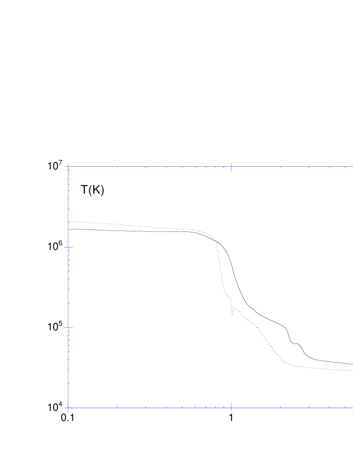
Figure 7.: Comparison of the temperature computed with (full line) and without (dashed lines) full eight-level He-like and full five-level Li-like ions, for the reference model, versus the distance to the illuminated side.

• First it should not predict correctly the details of the line spectrum, since it neglects subordinate lines and even important resonance lines.

• Also it can lead to a bad estimation of the energy losses and consequently to a change of the temperature. The recombination continuum corresponds generally to a smaller absorption coefficient than the neglected lines, and therefore can escape more easily from the deep layers. It would correspond to an overestimation of the losses and an underestimation of the temperature. But other parameters, such as the ionization state, play also a crucial role in the energy balance, so the net effect is difficult to predict. Fortunately in these models cooling due to lines is not predominant except in some regions.

• It can lead to important errors in the fractional ion abundances. This effect is “self-cumulating”, as an increased proportion of a given ion leads to a stronger ionization edge, which in turns inhibits further photoionizations. So again the net effect is not predictable.

• Finally recombinations onto excited levels are not balanced by ionizations from these levels. It is not important in conditions prevailing in a photoionized slab far from equilibrium (like for instance in the hot skin of an irradiated accretion disk), as the lowest atom levels are strongly overpopulated with respect to LTE. But this treatment is not valid in the innermost layers of a disk atmosphere, where the density is very high so complete LTE is almost reached.

We have recently introduced interlocked multi-level computations for He-like and Li-like ions, in order to obtain a better description of the spectrum, and to treat cases closer to LTE. However we are for the moment restricted to 8 levels for He-like ions and 5 for Li-like ones, which is not sufficient close to LTE. We take into account recombinations onto the levels higher than 8 for He-like ions (respectively 5 for Li-like), adding them as a contribution to the recombination of the highest level. This treatment is similar to the old one, except that it takes into account many subordinate lines and ionizations from excited levels, and it is valid as far as LTE is not reached for the highest levels and ionizations are dominated by the ground level. Like for hydrogen-like ions we plane to add several other levels, and to mimic the contributions of the higher levels.

We mention also that radiative recombinations are computed differently according to the relative values of $kT$ to the photon energy bin, in order to get an accurate frequency dependence.

Figs. 7 to 10 illustrate the influence of the new treatment with respect to the old one, for the reference model (except that the thickness is only $\tau_{\rm es}=25$ instead of 80; we have already mentioned that above this value nothing varies anymore for $\xi=10^{3}$, cf. Fig. 4). In this model the level populations and the ionization degrees are far from LTE, even in the deepest layers. It is quite comparable to a classical photoionized model, where excited levels are populated by radiative recombinations and depopulated by deexcitations onto lower levels. Note that these results are obtained with the new transfer treatment.

Fig. 7 shows the new temperature profile. Except at the surface $T$ is increased with respect to the previous computation. The change is quite important, reaching a factor two in the transition layer. Fig. 8 shows the change of fractional abundances of Hydrogen, Helium, and Iron. It is relatively important in the hot skin for HeI, but the abundance of this ion is completely negligible in this region, so it should not induce any change in the emitted spectrum around the ionization edge, i.e. 20 eV. The result of a computation with full He-like and Li-like atoms, but without additional recombinations on the highest level, is also shown. Except precisely for HeI in the hot skin, the results with and without the additional term are quite similar.

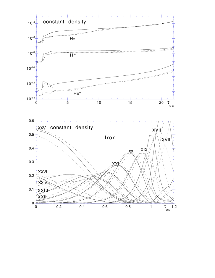
Figure 8.: Fractional abundances of Hydrogen, Helium and Iron, computed with (dotted line) and without (full lines) full eight-level He-like and full five-level Li-like ions, for the reference model, versus the distance to the illuminated side. The result of a computation with full He-like and Li-like atoms, but without additional recombinations on the highest level, is also shown (dashed lines).

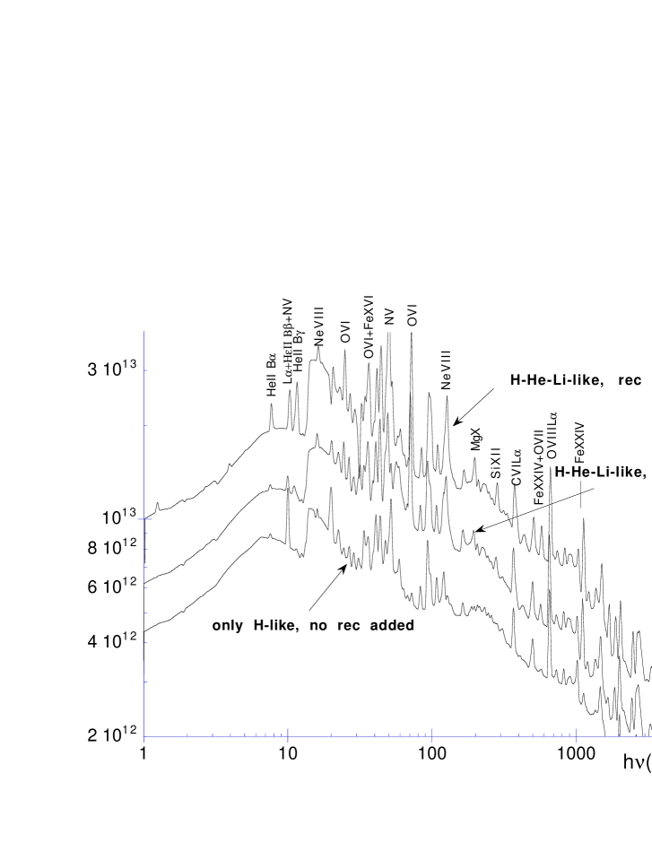
Figure 9.: Reflected spectrum computed with and without full eight-level He-like and full five-level Li-like ions, for the reference model. The result of a computation with full He-like and Li-like atoms, but without additional recombinations on the highest level, is also shown. The spectra are vertically shifted for a better reading. They are displayed with a resolution of 30. A few intense lines are identified.

Figure 10.: Reflected spectrum computed with and without full eight-level He-like and full five-level Li-like ions, for the reference model. The result of a computation with full He-like and Li-like atoms, but without additional recombinations on the highest level, is also shown. The spectra are vertically shifted for a better reading. They are displayed with a resolution of 100. A few intense lines are identified.

Figs. 9 and 10 display the reflected spectrum for this model, computed with the old and the new atomic treatment, with a low resolution in the whole energy range (Fig. 9), and with a higher resolution in a smallest but interesting energy range (Fig. 10).

The spectral distribution does not differ much for the two treatments. This is not the case of the detailed features, as it can be seen on Fig. 10. The flux of the main lines of H-like ions in the reflected spectrum are almost not changed (which is expected since the treatment is the same). For the He-like and Li-like ions, the total flux for all lines is multiplied by a factor 3 or 4. To illustrate this effect, Fig. 11 displays the fluxes of the OVI, OVII, and OVIII lines. Even the resonant lines differ in both treatments, as the energy is distributed among a much larger number of lines: for instance the OVIII line at 665 eV decreases by one order of magnitude with the new treatment. The net increase of line flux is simply due to the redistribution of continuum recombination photons into line photons through cascades, an effect which was only partly taken into account in the previous treatment.

Besides, we have added the result of a computation performed with the complete treatment of He-Li-like ions, when suppressing the recombination rates added on the highest level (cf. Figs. 9 and 10). This suppression does not affect at all the spectral distribution, and only slightly the detailed features of the spectrum.

The next further step is to introduce forbidden lines, which could be important for the cooling of the medium in some places.

Note that all the results given in the following sections are obtained without Li-like and He-like complete atom models.

4.2. Influence of the density distribution

Constant pressure

:

Up to now, we have presented results only for slabs of constant density. It is a peculiar case, as the pressure is thus varying according to the density and the temperature. When the pressure is imposed and not the density, one is faced to the well-known problem of thermal instability described first in the framework of AGN by Krolik, McKee & Tarter (1981). If the pressure is imposed, three (or even more) solutions to the Gain=Loss equation can exist, and one of these solutions is unstable. The gas has therefore to shift either to the Compton dominated hot solution at a temperature close to the Compton value, or to the cold solution dominated by atomic processes, at a few $10^{4}$ K.

Figure 11.: Line fluxes with (open symbols) and without (full symbols) full eight-level He-like and full five-level Li-like ions, for the reference model. OVI: circles; OVII: losanges; OVIII: squares.

Krolik et al. were considering optically thin media with a uniform temperature, whose value is given by the external irradiating spectrum. Here we are considering a stationary case, where the temperature changes across the slab because the mean intensity $J_{\nu}$ is modified as a function of depth. Since $J_{\nu}$ is absorbed in the soft X-ray band, its spectral distribution becomes more dominated by UV as the depth increases, and such a spectrum does not lead to the S-shape curve characteristic of thermal instability (cf. Krolik et al. 1981). However, even if there is no instability, the temperature decreases very rapidly with increasing depth, as the constancy of the pressure leads to an increase of the density, therefore to an increase of the cooling, and to a further decrease of temperature (note that the temperature is not strictly inversely proportional to the density, as radiation pressure generally exceeds gas pressure).

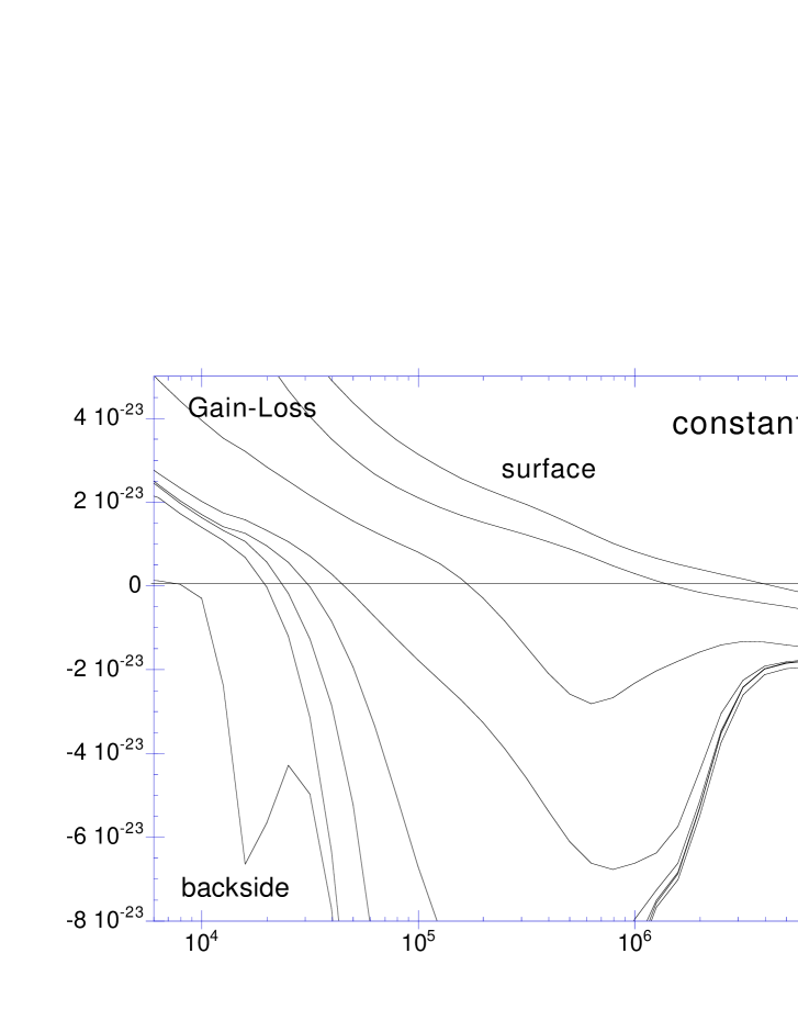
Figure 12.: Gain-Loss function versus the temperature, for different layers across the slab, for a constant pressure model.

This is illustrated on Fig. 12 which shows the Gain-Loss function versus the temperature for different layers. The model is a slab with a constant pressure, a density at the surface equal to 10¹¹ cm^-3, an ionization parameter equal to 1000. The illuminating spectrum is a power law $F_{\nu}\propto\nu^{-0.7}$, chosen because such a flat spectrum is well known to correspond to an “S-shape” curve with a strong instability. However we see that as the temperature decreases with the depth, there are never multiple solutions of the Gain=Loss equation. Note that it is by no means a general result. In particular, a medium with a more rapid variation of the pressure with the depth, like given by hydrostatic equilibrium, could likely lead to a thermal instability, as the transition to the cold region occurs in a region where the spectrum is less absorbed than in a constant density medium (cf. Nayakshin, Kazanas & Kallman 2000). Also if the UV band is absorbed before the soft X-ray one, which is the case when the ionization parameter is small, it should lead to a thermal instability.

Fig. 13 displays the temperature versus depth for slabs of constant density and slabs of constant pressure, with different ionization parameters. Note that it would be better to speak of “ionizing flux” instead of ionizing parameter in the constant pressure case. Actually the comparison is performed with the same incident fluxes. As expected, and in contrast with the constant density case where there is a smooth decrease of the temperature with increasing depth, the constant pressure case gives a sharp transition between the hot and dilute, and the cold and dense, parts of the slab. Moreover the thickness of the “hot skin” is smaller for the same flux in the constant pressure case, in particular for high illumination. For instance, for $\xi=10^{3}$ the Thomson thickness of the hot skin is about unity in the constant density case, and only 0.4 in the constant pressure case. All these effects have strong consequences on the emission spectrum.

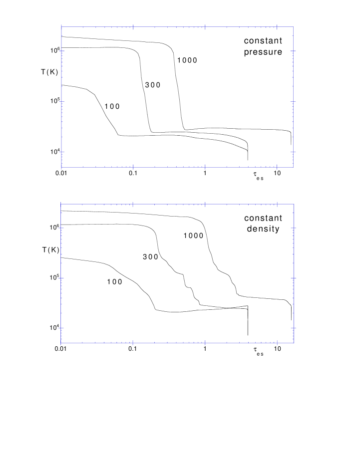
Figure 13.: Temperature versus depth for different values of $\xi$ in erg cm s^-1, for constant pressure and constant density. The constant density slabs have a density of $10^{12}$ cm^-3, and the density at the surface of the slab with constant pressure is equal to the same value. The other parameters are the same as in the reference model.

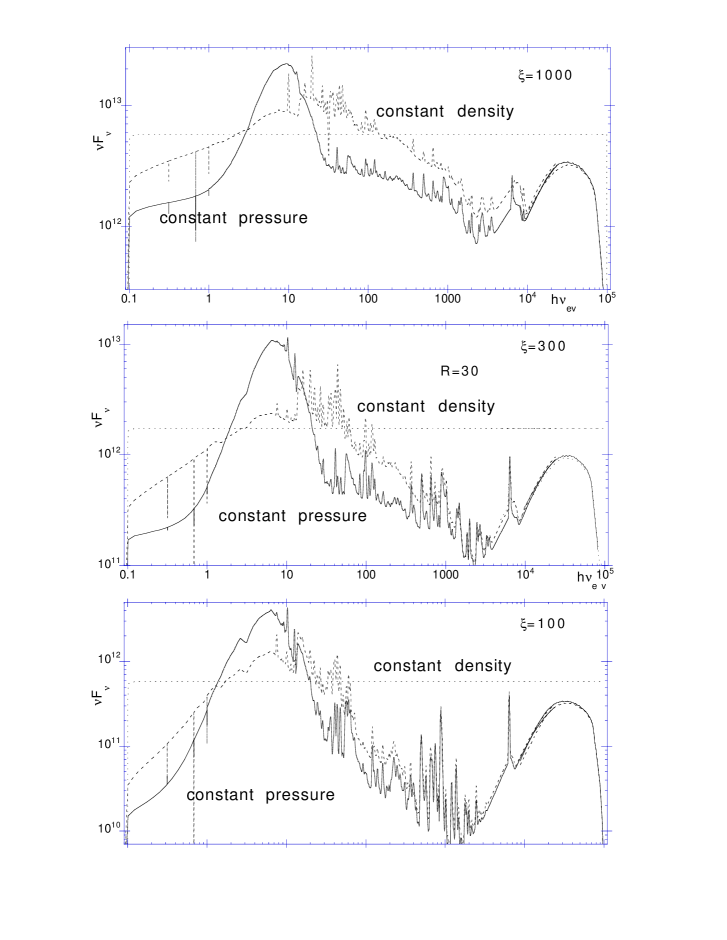
Figure 14.: Reflected spectra computed with constant pressure (full line) and with constant density (dashed lines) for the models of the previous figure; the spectra are displayed with a resolution of 30.

For constant pressure the spectrum displays a narrow UV bump, while the constant density the UV bump is more extended in frequency, as it corresponds to intermediate temperatures which do not exist in the constant pressure case (cf. Fig. 14). The difference between the two cases is particularly apparent for high illumination, as expected. It is interesting to note that the Lyman edge is quite weak in the constant pressure case, since the UV spectrum is closer to a blackbody. This is a point that constant density models have difficulties to account for in AGN.

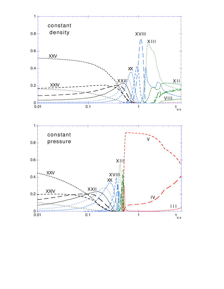
Figure 15.: Fractional abundances of iron versus depth, in the case of constant pressure or constant density slabs, for the incident flux $8.10^{13}$ erg cm^-2 s^-1 for one of the model of the previous figure ($\xi=1000$).

The distribution of fractional ionic abundances is also completely modified. As an illustration, Fig. 15 displays the fractional abundances of iron versus depth. The most remarkable difference is the presence at $\tau_{\rm es}\sim 1$ of low ionization species, such as FeIV or FeV, which are completely absent in the constant density case. One notes also that the extension of highly ionized species is smaller than in the constant density case, as expected. For instance FeXIV is present up to $\tau_{\rm es}=0.4$ for constant pressure, instead of $1.2$ for constant density. As a consequence, the Iron K lines produced are different from the constant density, as we shall see later.

Hydrostatic equilibrium

:

In order to describe an irradiated accretion disk, we have introduced in collaboration with A. Rosanska and B. Czerny a variation of the density given by the hydrostatic equilibrium law. TITAN treats then only the layer at the surface of the disc where the diffusion approximation does not hold. In this case there is a flux incident on the back side of the slab, equal to the flux generated by viscous dissipation inside the disk. Iterations are needed with the hydrostatic equilibrium equations (for more details see Różańska et al. 2001).

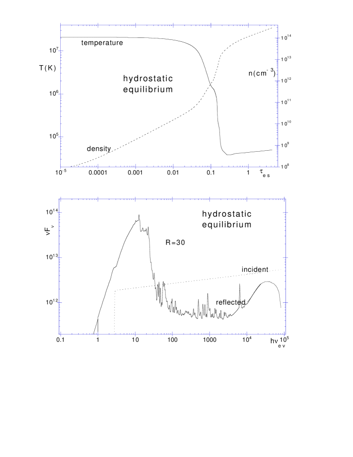
Figure 16.: Temperature versus depth, and reflected spectrum, obtained for an illuminated accretion disk in hydrostatic equilibrium, as described in the text. From Różańska et al., 2001.

Fig. 16 shows the results for the following case: $M_{\rm BH}=10^{8}$ M_⊙, $\dot{m}=0.03$, $R=10R_{\rm sch}$, and an X-ray irradiating powerlaw spectrum, with a spectral index 0.9 in flux, and an X-ray flux $F_{X}=3.5\times 10^{13}$, i.e. equal to half the viscous flux. Note that the temperature decreases abruptly like in the constant pressure case, and that the hot skin is very thin. The temperature reaches that given by viscous dissipation at about $\tau_{\rm es}=0.4$. The reflected spectrum displays a prominent blue bump with no soft X-ray excess, and a strong absorption in the UV range due to low ionization species in the deep layers of the atmosphere. It is important to note that such a spectrum differs strongly from that of an irradiated disc in which the density is assumed to be constant (Ross & Fabian 1993, and subsequent works, cf. Różańska et al. 2001 for a detailed discussion). Our results are similar to those of Nayakshin, Kazanas & Kallman (2000).

5. Coupling of TITAN and NOAR

5.1. Monte Carlo code NOAR

In order to compute the effect of Compton scattering on the high energy part of the reprocessed radiation and to determine precisely the Compton heating-cooling rate in the energy balance equation, one needs another numerical approach. In this aim Abrassart (1998) developed a Monte Carlo code, NOAR (cf. Dumont et al. 2000). The asset of such an approach is also that it enables to investigate an arbitrary geometry and to determine the angular dependence of the observed spectra. Moreover, it allows to easily extract time variability information.

NOAR takes into account direct and inverse Compton scattering, according to the method proposed by Pozdniakov, Sobol & Sunyaev (1983) and by Gorecki & Wilczewski (1984). Given all the fractional abundances and the temperature in each layer provided by TITAN, it computes the absorption cross sections in each layer. Free-free absorption is taken into account, as well as recombination continua of hydrogen and helium like ions (the spectral distribution of the recombination continuum is determined by the local temperature). The proper yields to account for the competition with the Auger effect are used for the fluorescence lines. Fluorescence of Iron XVII to XXIII is suppressed by resonant trapping (but not in TITAN). For the pseudo fluorescence of Iron XXV and XXVI, a simplifying prescription is adopted which includes the two most probable outcomes of a K shell photoionization, that is: direct recombination on ground level or L-K transition. Other line emission is not included.

One use of NOAR is to provide TITAN with the local Compton gains and losses in each layer. This is necessary, because Compton heating-cooling is dominated by energy losses of photons $>$ 20 keV for high values of $\xi$. In Dumont et al. (2000) it was shown that given an incident spectrum the dependence of the Compton heating-cooling over $\xi$ ratio on the Thomson depth depends only slightly on $\xi$ except for high values of $\xi$. The Compton heating-cooling rate obtained with NOAR is fitted analytically as a function of $z$, which is transferred to TITAN. The spectra computed with TITAN are then completed. (cf. Fig. 17, and also Figs. 14 and 16).

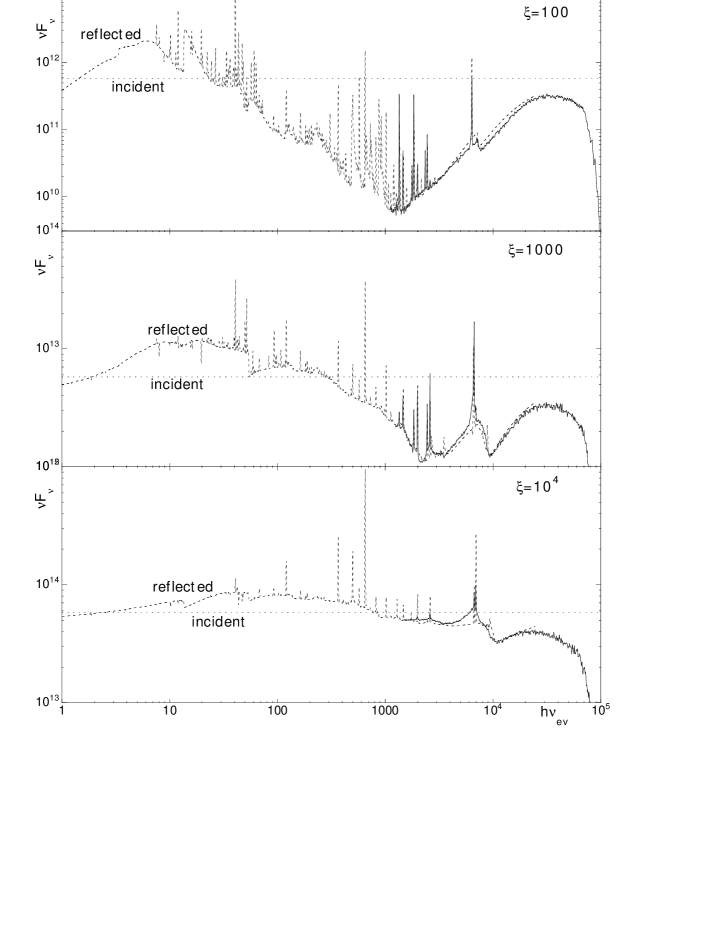
Figure 17.: Reflected spectrum for different values of $\xi$ in erg cm s^-1, the other parameters being the same as in the reference model; full lines: results of NOAR; dashed lines: results of TITAN. The spectra are displayed with a resolution of 100.

5.2. Some results of TITAN and NOAR

TITAN and NOAR lead to similar energy distributions of the reflected spectra in the 1-20 keV range. The reflected spectrum above 10 keV exhibits a “Compton hump” depending on the high energy cut-off of the incident spectrum, which is here 100 keV, and on the ionization parameter. The spectrum in the higher energy range is used for the energy balance.

Comptonisation leads also to line broadening, and when it is important, to smearing of the ionization edges. Direct Compton downscatterings produce a red wing, while inverse Compton upscatterings produce a blue wing. The effect can be comparable to relativistic broadening near the black hole, and can account partly for the broad profiles of the iron line in AGN (Abrassart & Dumont 1998).

Fig. 18 displays (with a relatively high resolution, in order to show detailed features) the spectrum around 7 keV in the constant density case, for different values of $\xi$, the other parameters being as in the reference model. The feature near 7 keV is made of a mixture of iron edges and of several iron lines:

- for $\xi$ equal to a few hundreds erg cm s^-1, the iron line is dominated by low ionization stages, smaller than iron XVII; the absorption edge is proeminent above 7 keV;

- for $\xi$ equal to $10^{3}$ erg cm s^-1, FeXXV and FeXXVI lines are apparent, modified by Compton scattering. The lines are significantly broadened, the broadening is asymmetric, the profile is skewed towards the red. The absorption edge is still important, but extends from 8 to 10 keV, due both to Comptonization and to the influence of several edges;

- for $\xi$ equal to $10^{4}$ erg cm s^-1, the line has a large red Compton wing and a weak blue wing, and it is weak. The absorption edge is completely erased.

Fig. 19 displays the iron line complex for the constant pressure case, to be compared to the constant density case. Both a “cold line” at 6.4 keV and FeXXV and XXVI lines are present in the constant pressure case, while only highly ionized species are visible in the constant density case. For constant pressure the cold layers are indeed closer from the surface than in the constant density case, so the photons emitted by these layers are able to leave the medium.

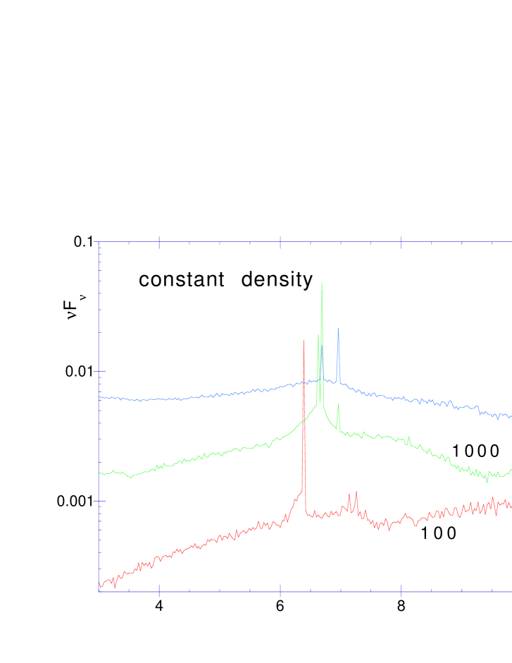
Figure 18.: Reflected spectrum around 7 keV for different values of $\xi$ in erg cm s^-1, the other parameters being the same as in the reference model; The broadening by Comptonization is important for $\xi>1000$ erg cm s^-1. The spectra are displayed with a resolution of 200.

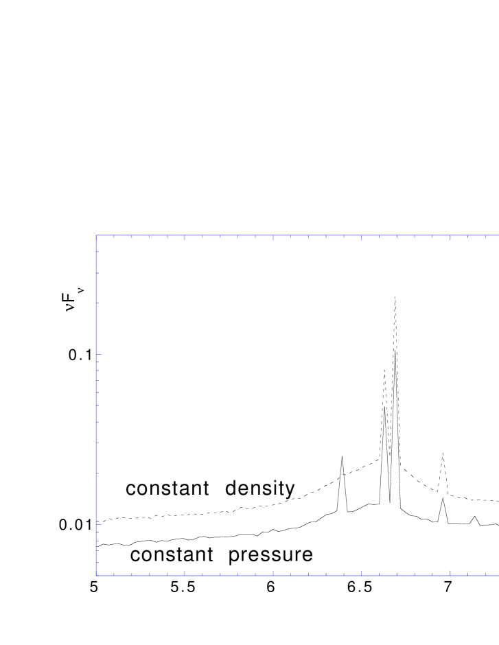
Figure 19.: Reflected spectrum in the X-range in the case of constant pressure or constant density slabs, for the incident flux $8.10^{13}$ erg cm^-2 s^-1. The spectra are displayed with a resolution of 200.

6. Foreseen improvements

The coupling of TITAN and NOAR allows to compute the structure and the emission of hot Compton thick irradiated media, by solving consistently the energy balance of the medium. Moreover it allows also to take into account Compton broadening of the lines and of the edges in the X-ray range.

In the previous description of the code (Dumont et al. 2000), we had already recalled the importance of the returning flux, which is often neglected, even for relatively low column densities, and we had compared the line transfer treatment for the lines with the escape probability approximation generally used in these problems. Here we have in addition stressed the influence of the pressure law, by showing the strong differences existing both in the structure and in the emitted spectrum, between a constant density medium, a constant pressure medium, or a medium in hydrostatic equilibrium. We have also shown that the atom models are of fundamental importance as they determine the ionization state, the energy balance, the temperature, and in fine the detailed spectral features which will be soon accessible through X-ray spectroscopy.

All along this paper we have mentioned what improvements we intend to bring to the code.

The Accelerated Lambda Iteration method is used now for the continuum. We will soon implement it for the lines, which are the most difficult to converge. It will in particular allow to treat partial redistribution in the lines.

In collaboration with S. Coupe and M.C. Artru (Coupe et al. 2001) we have begun to take into account subordinate lines for all ions by solving a complete multi-level atom for Li-like and He-like ions, after H-like ions which were already introduced in the previous version of the code. In the future we plan to implement other iso-electronic sequences, and to add to the present ones several other levels. In particular we will try to get a better representation of the highest levels for computations close to LTE. We will take into account forbidden lines, which could be important for the cooling of the medium in some places. We also intend to add to the line transfer an option allowing the UV and soft X-ray photons to escape from the medium through Compton scattering.

Though there are still many improvements to perform, we presently use these codes to model AGN spectra in the UV and X-ray range, in conditions where they are valid.

References

Abrassart A. & Dumont A.-M. 1998, Proceedings of the First XMM workshop on Science with XMM”, M. Dahlem (ed.)

Abrassart A. 1999, Proceedings of the 32nd Cospar Scientific Assembly, Nagoya, Japan, Advances in Space Research, Vol 25 issue/3-4, p 465

Auer H.L., Paletou F. 1994, A&A 284, 675

Canfield R.C., Ricchiazzi P.J. 1980, ApJ 239, 1036

Cannon C.J. 1973, J. Quant. Spectroscop. Radiat.Transfer 13, 627

Cunto W., Mendoza C., Ochsenbein F., Zeippen C.J. 1993, A&A 275, L5

Coupe S., Dumont A-M., Artru, M-C., Collin S. 2001, in preparation

Collin-Souffrin S., Czerny B., Dumont, A. M. & Zycki P.T. 1996, A&A 314, 393

Czerny B. & Dumont A.-M. 1998, A&A, 338, 386

Dumont A.-M., Abrassart A., Collin S. 2000, A&A 357, 823

Francis P.J., et al. 1991, ApJ 373, 465

Ferland G.J., Korista T., Verner D.A., Ferguson J.W., Kingdom J.B., Verner E.M., 1998, PASP 110, 761

Gorecki A., Wilczewski W. 1984, Acta Astronomica 34, 141

Krolik, J.H., McKee, C.F., Tarter, C. B., 1981, ApJ 249, 422

Kunasz P. & Auer H. L. 1988, J. Quant. Spectroscop. Radiat. Transfer 39, 67

Laor, A., Fiore, F., Elvis, M., Wilkes, B.J., McDowell, J.C. 1997, ApJ 477, 93

Ng K. C. 1974, J. Chem. Phys. 61, 2680

Olson G.L., Auer L.H., Buchler J.R. 1986, J. Quant. Spectroscop. Radiat. Transfer 35, 431

Pozdniakov L.A., Sobol I.M., Sunyaev R.A. 1983, Astrophysics and Space Physics Reviews 2, 189

Ross R.R., Fabian A.C., 1993, MNRAS 261, 74

Różańska A., Czerny B., Dumont A-M. Collin, S. 2001, A&nnnA, submitted

Zheng W., Kriss G.A., Telfer R.C., Grimes J.P., Davidsen A.F. 1997, ApJ 475, 469