Multiscale Gaussian Random Fields for Cosmological Simulations

Abstract

This paper describes the generation of initial conditions for numerical simulations in cosmology with multiple levels of resolution, or multiscale simulations. We present the theory of adaptive mesh refinement of Gaussian random fields followed by the implementation and testing of a computer code package performing this refinement called GRAFIC2. This package is available to the computational cosmology community at http://arcturus.mit.edu/grafic/ or by email from the author.

1 INTRODUCTION

Advances in computational algorithms combined with the steady advance of computer technology have made it possible to simulate regions of the universe with unprecedented dynamic range (Bertschinger, 1998). Realistic simulations of galaxy formation require spatial resolution better than 1 kpc and mass resolution better than $10^{6}\ M_{\odot}$ in volumes at least 100 Mpc across containing more than $10^{17}\ M_{\odot}$. Cosmologists have made significant progress towards these requirements. In simulations of dark matter halos, Fukushige & Makino (1997) and Ghigna et al. (2000) have achieved more than 4 orders of magnitude in spatial resolution while the Virgo Consortium has performed simulations with $10^{9}$ particles (Colberg et al., 2000). Recently, Abel et al. (2000) have performed a simulation of the formation of the first subgalactic molecular clouds using adaptive mesh refinement with a spatial dynamic range of 262,144 and a mass dynamic range more than $10^{16}$.

The possibility to resolve numerically such vast dynamic ranges of length and mass begs the question of what are the appropriate initial conditions for such simulations. Hierarchical structure formation models like the cold dark matter (CDM) family of models have increasing amounts of power at smaller scales. This power should be present in the initial conditions. For simulations of spatially constant resolution, this is straightforward to achieve using existing community codes (Bertschinger, 1995). However, workers increasingly are using multiscale methods in which the best resolution is concentrated in only a small fraction of the simulation volume. How should multiscale simulations be initialized?

Many workers currently initialize multiscale models following the approach of Katz et al. (1994). First, a Gaussian random field of density fluctuations (and the corresponding irrotational velocity field) is sampled on a Cartesian lattice of fixed spacing $\Delta x$. Then, $\Delta x$ is decreased by an integer factor $r>1$ and a new Gaussian random field is sampled with $r^{3}$ times as many points, such that the low-frequency Fourier components (up to the Nyquist frequency $\pi/\Delta x$ in each dimension) agree exactly with those sampled on the lower-resolution grid.

This method has two drawbacks. First, it is limited by the size of the largest Fast Fourier Transform (FFT) that can be performed, since the Gaussian noise is sampled on a uniform lattice in Fourier space. This represents a severe limitation for adaptive mesh refinement codes which are able to achieve much higher dynamic range. Second, the uniform high-frequency sampling on the fine grid is inconsistent with the actual sampling of the mass used in the evolutionary calculations. Multiscale simulations have grid cells, hence particle masses, of more than one size. The gravitational field produced by a distribution of unequal particle masses differs from that produced with constant resolution. In the linear regime, the velocity and displacement should be proportional to the gravitational field. With the method of Katz et al. (1994), they are not. We are challenged to develop a method for sampling multiscale Gaussian random fields consistent with the multiresolution sampling of mass.

A satisfactory method should satisfy several requirements in addition to correctly accounting for variable mass resolution. First, each refined field should preserve exactly the discretized long-wavelength amplitude and phase so as to truly refine the lower-resolution sample. Second, high-frequency power should be added in such a way that the multiscale fields are an exact sample from the power spectrum over the whole range of wavelengths sampled. Because multiscale fields are not sampled on a uniform lattice, it is not the power spectrum but rather than spatial two-point correlation function that should be exactly sampled. Finally, a practical method should have a memory requirement and computational cost independent of refinement so that it is not limited by the size of the largest FFT that can be performed.

This paper presents the analytic theory and practical implementation of multiscale Gaussian random field sampling methods that meet these requirements. Our algorithms are the equivalent of adaptive mesh refinement applied to Gaussian random fields. The mathematical properties of such fields are simple enough so that an exact algorithm may be developed. Practical implementation requires certain approximations to be made but they can be evaluated and the errors controlled.

The essential idea enabling this development is that Gaussian random fields can be sampled in real space rather than Fourier space (hereafter $k$-space). Adaptive mesh refinement can then be performed in real space conceptually just as it is done in the nonlinear evolution code used by Abel et al. (2000).

How can the long-range correlations of Gaussian random fields be properly accounted for in real space? In an elegant paper, Salmon (1996) pointed out that any Gaussian random field (perhaps subject to regularity conditions such as having a continuous power spectrum) sampled on a lattice can be written as the convolution of white noise with a function that we will call the transfer function. Salmon recognized the advantages of multiresolution initial conditions and developed a tree algorithm to perform the convolutions. Tree algorithms have the advantage that they work for any mesh—regular, hierarchical, or unstructured.

Next, Pen (1997) pointed out that FFTs may be used to perform the convolutions in such a way that the two-point correlations of the sampled fields are exact, in contrast with the usual $k$-space methods which produce exact power spectra but not two-point correlations. The key is that the transfer functions may be evaluated in real space accurately at large separation free from distortions caused by the discretization of $k$-space. Pen also pointed out that this method allows the mean density in the box to differ from the cosmic average, and that the method could be extended to hierarchical grids.

This paper builds upon the work of Salmon (1996) and Pen (1997) as well as the author’s earlier COSMICS package (Bertschinger, 1995), which included a module called GRAFIC (Gaussian Random Field Initial Conditions). GRAFIC implemented the standard $k$-space sampling method for generating Gaussian random fields on periodic rectangular lattices. This paper presents the theory and computational methods for a new package for generating multiscale Gaussian random fields for cosmological initial conditions called GRAFIC2. This paper contains the fine print for the owner’s manual to GRAFIC2, as it were.

This paper is organized as follows. §2 reviews the mathematical method for generating Gaussian random fields through convolution of white noise including adaptive mesh refinement. §2.4 presents methods for the all-important computation of transfer functions. §3 presents important details of implementation. Exact sampling requires careful consideration of both the short-wavelength components added when a field is refined (§3.1) as well as the long-wavelength components interpolated from the lower-resolution grid (§3.2). As we show, the long-wavelength components must be convolved with the appropriate anti-aliasing filter. Truncation of this filter to a subvolume (a step required to avoid intractably large convolutions) introduces errors that we analyze and reduce to the few percent level in §3.4.

The method is extended to hierarchical grids in §4. §5 presents additional tricks with Gaussian random fields made possible by the white noise convolution method. §6 summarizes results and describes the public distribution of the computer codes developed herein for multiscale Gaussian random fields.

2 MATHEMATICAL METHOD

The starting point is the continuous Fourier representation of the density fluctuation field:

$$\delta(\vec{x}\,)=\int d^{3}k\,e^{i\vec{k}\cdot\vec{x}}\,T(k)\xi(\vec{k}\,)\ ,$$ (1)

where $\xi(\vec{x}\,)$ is Gaussian white noise with power spectrum

$$\left\langle\xi(\vec{k}_{1})\xi(\vec{k}_{2})\right\rangle=\delta_{\rm D}^{3}(\vec{k}_{1}+\vec{k}_{2})\ .$$ (2)

Here $\delta_{\rm D}(\vec{k}\,)$ is the Dirac delta function and we are assuming that space is Euclidean. The function $T(k)$ is the transfer function relative to white noise, and it is related simply to the power spectrum of $\delta(\vec{x}\,)$:

$$T(k)=[P(k)]^{1/2}\ .$$ (3)

Note that $\xi(\vec{k}\,)$ and $T(k)$ both have units of $[\hbox{length}]^{3/2}$ and that $T(k)$ is an ordinary function while $\xi(\vec{k}\,)$ is a stochastic field (a distribution).

The next step is to recognize that equation (1) can be written as a convolution (Salmon, 1996):

$$\delta(\vec{x}\,)=(\xi\ast T)(\vec{x}\,)=\int d^{3}x^{\prime}\,\xi(\vec{x}^{\,\prime})T(|\vec{x}-\vec{x}^{\,\prime}|)$$ (4)

where

$$T(|\vec{x}\,|)=\int{d^{3}k\over(2\pi)^{3}}\,e^{i\vec{k}\cdot\vec{x}}\,T(k)$$ (5)

and

$$\left\langle\xi(\vec{x}_{1})\xi(\vec{x}_{2})\right\rangle=(2\pi)^{3}\delta_{\rm D}^{3}(\vec{x}_{1}-\vec{x}_{2})\ .$$ (6)

The spatial two-point correlation function of $\delta(\vec{x}\,)$ is simply $(2\pi)^{3}(T\ast T)(\vec{x}\,)$.

Thus, we may construct an arbitrary Gaussian random field by the convolution of white noise with a convolution kernel determined by the power spectrum. The white noise process is formally divergent; from equation (6), $\xi(\vec{x}\,)$ is drawn from a Gaussian distribution with infinite variance. This strange behavior arises because we are including contributions from all scales and $\xi(\vec{x}\,)$ is ultraviolet-divergent. Physically this divergence may be cut off by the power spectrum, although the standard cold dark matter spectrum still leads to a logarithmic divergence of the dark matter density fluctuations at small scales. In practice the integral is cut off at high wavenumber by discretizing space with a finite cell size.

The standard method for generating Gaussian random fields relies on discretizing equation (1) with a Cartesian mesh in a finite parallelpiped with periodic boundary conditions. The spatial dynamic range is then limited by the size of the largest FFT that can be performed. The Fourier domain is used because the random variables at different points are statistically independent aside from the condition $\xi(-\vec{k}\,)=\xi^{\ast}(\vec{k}\,)$ required to enforce reality of $\delta(\vec{x}\,)$. In the spatial domain, $\delta(\vec{x}\,)$ has long-range correlations that are difficult to sample unless one first goes to Fourier space.

The velocity field (or displacement field, in the case of dark matter particles) obeys similar equations; only the transfer function $T(k)$ is modified.

The convolution method described in this paper evaluates the density and velocity fields using equation (4) instead of equation (1). It relies on the fact that white noise is uncorrelated in the spatial domain as well as the Fourier domain, hence there is no difficulty in sampling $\xi(\vec{x}\,)$. Once we have such a sample, it is unnecessary to use a single enormous FFT to evaluate the convolution equation (4). Tree algorithms may be used (Salmon, 1996) or multiple FFTs with appropriate boundary conditions (Pen, 1997). The algorithm we develop extends the ideas of Pen.

2.1 Discrete Convolution Method Without Refinement

The heart of our method lies in the discretization of equations (1)-(6) and their application to density fields with spatially variable resolution. The density field is represented on a hierarchy of nested Cartesian grids so that FFT methods can be used to perform the convolutions.

Before describing convolution with spatially variable resolution, we first describe the discrete convolution method for a single grid of $M$ points per dimension. For simplicity of presentation we assume here a cube of length $L$ with periodic boundary conditions, although the code that implements the convolution is generalized to allow any parallelpiped. The grid positions are $\vec{x}(\vec{m}\,)=(L/M)\vec{m}$ where $\vec{m}$ is an integer triplet with components $m_{i}\in[0,M)$. Equation (1) becomes

$$\delta(\vec{m}\,)=\sum_{\vec{\kappa}}\exp\left({i2\pi\over M}\vec{\kappa}\cdot\vec{m}\right)T(k)\xi(\vec{k}\,)$$ (7)

where $\vec{\kappa}=\vec{k}L/(2\pi)$ is the dimensionless wavenumber; it is an integer or half-integer triplet with components $\kappa_{i}\in[-M/2,M/2)$. The dimensionless transfer function and spectral noise appearing in equation (7) are given by

$$T(k)\equiv\left[(2\pi/L)^{3}P(k)\right]^{1/2},\ \ \xi(\vec{k}\,)=M^{-3}\sum_{\vec{m}}\exp\left(-{i2\pi\over M}\vec{\kappa}\cdot\vec{m}\,\right)\,\xi(\vec{m}\,)\ ,$$ (8)

where $\xi(\vec{m}\,)$ is white noise with variance $M^{3}$:

$$\left\langle\xi(\vec{m}_{1})\xi(\vec{m}_{2})\right\rangle=M^{3}\delta_{\rm K}(\vec{m}_{1},\vec{m}_{2})=M^{3}\times\cases{1\ ,&$\vec{m}_{1}=\vec{m}_{2}$;\cr 0\ ,&$\vec{m}_{1}\neq\vec{m}_{2}$\ .\cr}$$ (9)

The subscript K denotes the Kronecker delta.

The discrete convolution algorithm proceeds through the following steps.

1. Sample $\xi(\vec{m}\,)$ by generating independent, zero-mean normal deviates with variance $M^{3}$ at each spatial grid point.

2. Use the FFT algorithm to evaluate the second of equations (8).

3. Multiply $\xi(\vec{k}\,)$ by the discrete transfer function $T(k)$.

4. Use the FFT algorithm to evaluate equation (7).

The result is a discrete approximation to equation (1).

So far, this method is identical to the usual one for generating Gaussian random fields (Bertschinger, 1995) except that an extra FFT is introduced by sampling $\xi(\vec{m}\,)$ in real space instead of Fourier space. This requires more computation but is crucial when we extend the method to a multiscale hierarchy, which we do next.

2.2 Mesh Refinement

Figure 1: An example of mesh refinement with two levels. The coarse grid has size $M=9$, the subvolume has size $M_{s}=3$, and the refinement factor is $r=4$.

Suppose that we have two-level grid hierarchy as shown in Figure 1. Now the spatial grid point positions in the refined volume are given by two integer triplets, $\vec{m}$ for the coarse grid and $\vec{n}$ for the subgrid:

$$\vec{x}(\vec{m},\vec{n}\,)=\vec{x}_{o}+\left(L\over M\right)\left(\vec{m}+{1\over r}\vec{n}\,\right)\ .$$ (10)

The subgrid is refined by an integer factor $r>1$, with $n_{i}\in[0,r)$. An offset $\vec{x}_{o}=-(r-1)L/(2rM)(1,1,1)$ is applied to center the refinement. As a result of mesh refinement, each coarse grid cell is split up into $r^{3}$ subcells.

Suppose that we already have a sample of white noise on the coarse grid, $\xi_{0}(\vec{m}\,)$. Convolution by the appropriate transfer function using equations (7) and (8) then gives the density field $\delta(\vec{m}\,)$. To refine the sampling, we generate a mesh-refined white-noise sample $\xi(\vec{m},\vec{n}\,)$ and convolve it with a higher-resolution transfer function.

The refined white-noise sample $\xi(\vec{m},\vec{n}\,)$ should retain the same low-frequency structure as the coarse-grid sample $\xi_{0}(\vec{m}\,)$. We ensure this by choosing $\xi(\vec{m},\vec{n}\,)$ to be a sample of Gaussian white noise subject to the linear constraint

$$\sum_{\vec{n}}\xi(\vec{m},\vec{n}\,)=r^{3}\xi_{0}(\vec{m}\,)\ .$$ (11)

The constraint is easy to apply using the Hoffman-Ribak algorithm (Hoffman & Ribak, 1991). One simply generates an unconstrained white noise sample $\xi_{1}(\vec{m},\vec{n}\,)$ with variance $(rM)^{3}$ and then applies a linear correction to enforce equation (11):

$$\xi(\vec{m},\vec{n}\,)=\xi_{1}(\vec{m},\vec{n}\,)+\xi_{0}(\vec{m}\,)-\bar{\xi}_{1}(\vec{m}\,)\ \ \hbox{where}\ \ \bar{\xi}_{1}(\vec{m}\,)\equiv r^{-3}\sum_{\vec{n}}\xi_{1}(\vec{m},\vec{n}\,)\ .$$ (12)

The sample so generated is Gaussian white noise satisfying the constraint equation (11) and having the desired covariance

$$\left\langle\xi(\vec{m}_{1},\vec{n}_{1})\xi(\vec{m}_{2},\vec{n}_{2})\right\rangle=(rM)^{3}\delta_{\rm K}(\vec{m}_{1},\vec{m}_{2})\delta_{\rm K}(\vec{n}_{1},\vec{n}_{2})\ .$$ (13)

Equation (12) has a simple interpretation. Mesh refinement takes place by splitting each coarse cell (labelled by $\vec{m}\,$) into $r^{3}$ subcells. The coarse-grid white noise value $\xi_{0}$ is first spread to each of the subcells, then a high-frequency correction $\xi_{1}-\bar{\xi}_{1}$ is added.

2.3 Subgrid Convolution

Our method requires performing several convolutions over the subgrid. In this subsection we describe the method for a generic high-resolution convolution, which is first expressed in Fourier space as follows:

$$\delta(\vec{m},\vec{n}\,)=\sum_{\vec{k}}\exp[i\vec{k}\cdot\vec{x}(\vec{m},\vec{n}\,)]\,T(k)\xi(\vec{k}\,)\ .$$ (14)

The sum is taken over the extended Fourier space of size ($rM)^{3}$. This Fourier space extends to wavenumbers $r$ times greater than that of equation (7). We can write the wavevector using two integer (or half-integer) triplets, $\vec{\kappa}$ and $\vec{b}$:

$$\vec{k}=\left(2\pi\over L\right)\left(\vec{\kappa}+M\vec{b}\,\right)$$ (15)

where $\kappa_{i}\in[-M/2,M/2)$ and $b_{i}\in[-(r-1)/2,(r-1)/2]$. The set of all $\vec{\kappa}$ for a given $\vec{b}$ is called a Brillouin zone. The coarse grid corresponds to the fundamental Brillouin zone, $\vec{b}=(0,0,0)$. Mesh refinement extends the coverage of wavenumber space by increasing the number of Brillouin zones to $r^{3}$ where $r$ is the refinement factor.

The major technical challenge of our algorithm is to perform the convolution of equation (14) without storing or summing over the entire Fourier space. This is possible when $\delta(\vec{m},\vec{n}\,)$ is required over only a subgrid in the spatial domain. The first step is to note that equation (14) is equivalent to

$$\delta(\vec{m},\vec{n}\,)=\sum_{\vec{m}^{\prime},\vec{n}^{\,\prime}}\xi(\vec{m}^{\,\prime},\vec{n}^{\,\prime})T(\vec{m}-\vec{m}^{\,\prime},\vec{n}-\vec{n}^{\,\prime})$$ (16)

where

$$\xi(\vec{m},\vec{n}\,)=\sum_{\vec{k}}\exp[i\vec{k}\cdot\vec{x}(\vec{m},\vec{n}\,)]\,\xi(\vec{k}\,)\ ,\quad T(\vec{m},\vec{n}\,)=(rM)^{-3}\sum_{\vec{k}}\exp[i\vec{k}\cdot\vec{x}(\vec{m},\vec{n}\,)]\,T(k)\ .$$ (17)

Now, mesh refinement is performed only over the subgrid of size $(rM_{\rm s})^{3}$ where $M_{\rm s}<M$, so it is not necessary to evaluate $\xi(\vec{m},\vec{n}\,)$ and $T(\vec{m},\vec{n}\,)$ for all $(rM)^{3}$ high-resolution grid points. We set $\xi(\vec{m},\vec{n}\,)=0$ outside of the subgrid volume. Consequently, $T(\vec{m},\vec{n}\,)$ needs to be evaluated only to distances of $\pm rM_{\rm s}$ grid points in each dimension in order that all contributions to $\delta(\vec{m},\vec{n}\,)$ be included. We will describe how the transfer functions $T(\vec{m},\vec{n}\,)$ are computed in the next subsection.

The function $\xi(\vec{m},\vec{n}\,)$ must also be evaluated on the subgrid. Because this is a sample of white noise, we simply draw independent real Gaussian random numbers with zero mean and variance $(rM)^{3}$ at each grid point. Subtracting a mean over coarse grid cells (eq. 12) or imposing any other desired linear constraints (using the Hoffman-Ribak method) is easily accomplished.

Once we have $\xi(\vec{m},\vec{n}\,)$ and $T(\vec{m},\vec{n}\,)$ on the subgrid, the next step is to Fourier transform them. For simplicity in presentation, let us suppose that the subgrid is cubic with $N_{\rm s}=(2rM_{\rm s})^{3}$ where $M_{s}$ is the number of coarse grid points that are refined in each dimension. The result is

$$\xi^{\prime}(\vec{k}^{\,\prime})={1\over N_{\rm s}}\sum_{\vec{x}}\exp-(i\vec{k}^{\,\prime}\cdot\vec{x}\,)\,\xi(\vec{x}\,)\ ,\quad T^{\prime}(\vec{k}^{\,\prime\,})=\sum_{\vec{x}}\exp(-i\vec{k}^{\,\prime}\cdot\vec{x}\,)\,T(\vec{x}\,)$$ (18)

where the sums are taken over the fine grid points in the subvolume, which has been doubled to the accommodate periodic boundary conditions required by Fourier convolution. Primes are placed on the wavevectors and on the transformed quantities to distinguish them from the original quantities $\xi(\vec{k}\,)$ and $T(k)$. Note that the sampling of $k$-space is different in equations (17) and (18) because the length of the spatial grid has changed from $L$ to $(2M_{s}/M)L$. Also, $T^{\prime}(\vec{k}^{\,\prime\,})$ is in general not spherically symmetric even if $T(\vec{k}\,)$ is spherical.

The final step is to perform the convolution by multiplication in the subgrid $k$-space followed by Fourier transformation back to real space:

$$\delta(\vec{x}\,)=\sum_{\vec{k}^{\,\prime}}\exp(i\vec{k}^{\,\prime}\cdot\vec{x})\,T^{\prime}(\vec{k}^{\,\prime\,})\xi(\vec{k}^{\,\prime})\ .$$ (19)

The reader may verify that equations (18) and (19) give results identical to equations (14) and (16), when $\xi(\vec{x}\,)$ is zero outside of the subvolume. Thus, we have achieved the equivalent of convolution on a grid of size $(rM)^{3}$ by using a (typically smaller) grid of size $(2rM_{s})^{3}$. Note well that $T^{\prime}$ is not the same as $T$, because it is based on spatially truncating $T(\vec{m},\vec{n}\,)$ and making it periodic on a grid of size $(2M_{s}/M)L$ instead of $L$.

So far the method looks straightforward. However, some practical complications arise which will discuss later, in the computation of the transfer functions in real space (§2.4) and in the split of our random fields into long- and short-wavelength parts on the coarse and fine grids, respectively (§3.2).

Finally, we note that we will perform the convolution of equation (14) using a grid of size $2rM_{s}$ in each dimension in the standard way using FFTs without requiring periodic boundary conditions for the subgrid of size $rM_{s}$. We calculate the transfer functions in the first octant of size $(rM_{s})^{3}$ and then reflect them periodically to the other octants using reflection symmetry (odd along the direction of the displacement, otherwise even). In order to achieve isolated boundary conditions, the white noise field is filled in one octant and set to zero in the other octants. If we desire to have periodic boundary conditions (e.g. for testing), we can set $M_{s}=M/2$ and fill the full refinement grid of size $(2rM_{s})^{3}$ with white noise.

2.4 Computation of Transfer Functions

The convolution method requires calculating the transfer functions $T(\vec{x}\,)$ for density, velocity, etc., on a high resolution grid $\vec{x}(\vec{m},\vec{n}\,)$ of extent $\pm rM_{s}$ grid points in each dimension. The transfer function is given in the continuous case by equations (3) and (5) and in the discrete case by the first of equations (8) and the second of equations (17). Our challenge is to compute the transfer functions on the subgrid without performing an FFT of size $(rM)^{3}$, under the assumption that the problem is too large to fit in the available computer memory. Also, we wish to avoid a naive summation of the second of equations (17), which would require $O(r^{6}M_{s}^{3}M^{3})$ operations. In practice, $r$ will be a modest-size integer (from 2 to 8, say) while $M_{s}$ will be much larger, of order $M/r$.

We present three solutions to this challenge. The first two are based, respectively, on three-dimensional discrete Fourier transforms while the third is based on a spherical transform.

2.4.1 Exact Method

The first method is equivalent to the second of equations (17) and is therefore exact in the sense of yielding the same transfer functions as if we had used full resolution on a grid of size $(rM)^{3}$. Note that Pen (1997) would call this method approximate because, after the FFT to the spatial domain, the results differ from the exact spatial transfer function of equation (5). We will say more about this in §2.4.3, but note simply that the discretization of $k$-space required for the FFT makes it impossible for the transfer function to be exact in both real space and $k$-space. The transfer function of this subsection is exact in $k$-space and is equivalent to the usual $k$-space sampling method.

We rewrite the second of equations (17) as

$$T(\vec{m},\vec{n}\,)=\sum_{\vec{\kappa}}e^{i(2\pi/M)\vec{\kappa}\cdot\vec{m}}\,T(\vec{\kappa},\vec{n}\,)\ ,$$ (20)

where

$$T(\vec{\kappa},\vec{n}\,)=(rM)^{-3}\sum_{\vec{b}}\exp\left[i\left(2\pi\over rM\right)(\vec{\kappa}+M\vec{b}\,)\cdot\vec{n}\,\right]\,T(\vec{k}\,)\ .$$ (21)

The Fourier space is split into Brillouin zones according to equation (15). Beware that the symbol $T$ has three different uses here which are distinguished by its arguments: it is either the transfer function in real space $T(\vec{m},\vec{n}\,)$, the transfer function in Fourier space $T(\vec{k}\,)$, or else the mixed Fourier/real case $T(\vec{\kappa},\vec{n}\,)$.

Equation (20) is a simple FFT of size $M^{3}$. This is the same size as is used for generating the coarse grid initial conditions, so it is tractable. However, we save the results only at those coarse grid points $\vec{m}$ that lie in the refinement subvolume, discarding the rest. By performing some unnecessary computation, the FFT reduces the number of operations required to compute this sum for all $\vec{n}$ from $O(M_{s}^{3}M^{3})$ to $O(r^{3}M^{3}\log M)$, a substantial savings.

Equation (21) is also a FFT, in this case of size $r^{3}$. However, we cannot evaluate both equations (20) and (21) using FFTs without storing $T(\vec{\kappa},\vec{n}\,)$ for all $(rM)^{3}$ points. In order to reduce the storage to a tractable amount (no more than the larger of $M^{3}$ and $8r^{3}M_{s}^{3}$), we must perform an outer loop over $\vec{n}$ to evaluate $T(\vec{m},\vec{n}\,)$. For each $\vec{n}$, we must compute $T(\vec{\kappa},\vec{n}\,)$ for all $\vec{\kappa}$, requiring direct summation in equation (21). The operations count for all $\vec{n}$ is then $O(r^{6}M^{3})$, which dominates over the $O(r^{3}M^{3}\log M)$ for equation (20). The operations count for equation (21) can be reduced by a factor of up to 6 by using symmetries when $T(\vec{k}\,)$ is spherically or azimuthally symmetric. Nonetheless, if we use this method, computation of the transfer functions is generally the most costly part of the whole method.

2.4.2 Minimal $k$-space Sampling Method

If the transfer function falls off rapidly with distance in real space, there is another way to evaluate $T(\vec{m},\vec{n}\,)$ that is much faster. It is based on noting that the Fourier sum is an approximation to the Fourier integral, and another approximation is given by simply changing the discretization in $k$-space. In equation (17), the step size in $k$-space is $2\pi/L$ where $L$ is the full size of the simulation volume. If we increase this step size to $(M/2M_{s})2\pi/L$, the transfer function $T(\vec{k}\,)$ will be evaluated with exactly the sampling needed for $T^{\prime}(\vec{k}^{\,\prime\,})$ in equation (19). In this case we don’t even need to transform $T(\vec{k}\,)$ to the spatial domain, truncate and periodize on the subgrid to give $T(\vec{m},\vec{n}\,)$, and then transform back to get $T^{\prime}(\vec{k}^{\,\prime\,})$. We simply replace $T^{\prime}$ with $T$ in Fourier space. This is exactly equivalent to decreasing the $k$-space resolution in equation (17) to the minimum needed to sample $T(\vec{m},\vec{n}\,)$ on the subgrid.

This method is extremely fast but its speed comes with a cost. Low wavenumbers are sampled poorly compared with equations (20) and (21), and the transfer functions are truncated in a cube of size $(2M_{s}/M)L$ instead of $L$. The decreased $k$-space sampling leads to significant real-space errors for distances comparable to the size of the box. This may be tolerable for the density but is unacceptable for the velocity transfer function. In §3.2 we will introduce anti-aliasing filters for the coarse grid for which the minimal $k$-space sampling method is well-suited. In §4 we will revisit the use of the minimally sampled transfer function for the density field.

2.4.3 Spherical Transform Method

Another fast method can be used when $T(\vec{k}\,)$ is spherically symmetric, as it is for the density and the radial component of displacement. In this case we approximate the second of equations (17) as a continuous Fourier integral,

$$T(\vec{x}\,) \approx (rM)^{-3}\int{d^{3}k\over(\Delta k)^{3}}\,e^{i\vec{k}\cdot\vec{x}}\,T(k)$$ (22)

$$= \left(L\over 2\pi rM\right)^{3}\int{\sin kr\over kr}\,T(k)\,4\pi k^{2}dk$$

$$= \left(L\over 2\pi rM\right)^{3}{2\pi\over r}\,\hbox{{\cal I}m}\!\int_{-\infty}^{\infty}kT(k)e^{ikr}\,dr\ .$$

Aside from units, this is essentially the same as equation (5). The last integral in equation (22) can be performed by truncating the Fourier integral at the Nyquist frequency of the subgrid, $k_{\rm Ny}=\pi rM/L$ and then using a one-dimensional FFT. The method is much faster than equations (20) and (21).

The Fourier integral of equation (22) can be evaluated accurately, yielding an essentially exact transfer function in real space. This approach was advocated by Pen (1997). However, this is not necessarily the best approach for cosmological simulations with periodic boundary conditions. In order to achieve periodic boundary conditions, such simulations compute the gravitational fields with $k$-space discretized at low frequencies as in the second of equations (17). In this case it would be inconsistent to use equation (22) on the top-level grid with periodic boundary conditions—the displacement field would not be proportional, in the linear regime, to the gravity field computed by the Poisson solver of the evolution code. However, the spherical method is satisfactory for refinements without periodic boundary conditions.

2.4.4 Anisotropic Transfer Functions

In order to use equation (22), the transfer function must be spherically symmetric. This seems natural for the density field given that the power spectrum $P(k)$ is isotropic. However, the standard FFT-based method for computing samples of the density field violates spherical symmetry through the Cartesian discretization of $k$-space. As we noted above, periodic boundary conditions are inconsistent with spherical symmetry on the largest scales. Moreover, the displacement transfer function is multiplied by a factor $i\vec{k}/k^{2}$ which breaks spherical symmetry for each Cartesian component.

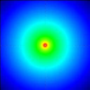
Figure 2: A slice through the center of the density transfer function in real space (“square root of the correlation function”). The exact method of §2.4.1 has been used with an unfiltered power spectrum. The cosmological model is flat $\Lambda$CDM and the box is 64 Mpc across. False colors are scaled to the logarithm of the transfer function, which shows 6 orders of magnitude. Anisotropy of the discrete Fourier transform leads to anisotropic features that are barely visible along horizontal and vertical axes through the center.

To examine the first concern, namely the non-isotropic discretization in Fourier space, we examine the transfer function computed using the exact method of §2.4.1. Figure 2 shows the result for the flat $\Lambda$CDM model ($\Omega_{\Lambda}=0.65$, $h=0.65$, $\sigma_{8}=1.0$) with a $r=4$ refinement of a $M_{\rm s}=32$ subgrid of a $M=256$ grid. The coarse grid spacing is 1 Mpc. In effect, the transfer function has been computed at $1024^{3}$ resolution on a grid of spacing 0.25 Mpc, but is shown only within a central region 64 Mpc across ($2M_{\rm s}\times\hbox{1 Mpc}$).

There is a slight banding visible along the $x$- and $y$-axes in Figure 2. The amplitude of this banding ranges from a relative size of about 20% at small $r$ to more than a factor of two at the edges (where the transfer function is very small); however, it is much smaller away from the coordinate axes. This anisotropic structure arises because, although $T(k)$ is spherically symmetric, the Fourier integration is not carried out over all $\vec{k}$ but rather only within a cube of size $2\pi rM/L$. The Fourier space is periodic (because the real space is discrete), which breaks the spherical symmetry of $T(\vec{x}\,)$. In this case it is the anisotropy at large $k$ that produces the anisotropy in real space.

This anisotropy is present in the initial conditions generated with the with the COSMICS package (Bertschinger, 1995). The author’s rational for allowing it was that it is preferable to retain all the power present in the initial density fluctuation field. Including all power in the Fourier cube gives the best possible resolution at small scales while producing a modest anisotropy along the coordinate axes. However, the effects of the anisotropy are unclear and should be more carefully evaluated. In §3.1, we will show how the density transfer function can be made isotropic by filtering. To determine whether the anisotropy of unfiltered initial conditions causes any significant errors, full nonlinear numerical simulations should be performed with and without filtering. That test is beyond the scope of this paper.

Additional considerations arise when calculating the transfer function for the linear velocity or displacement fields. (The linear velocity and displacement are proportional to each other.) The displacement field $\vec{\psi}(\vec{x}\,)$ is related to the density fluctuation field by $\vec{\nabla}\cdot\vec{\psi}=-\delta(\vec{x}\,)$ in real space or $\vec{T}_{\psi}(\vec{k}\,)=(i\vec{k}/k^{2})T(k)$ in $k$-space. Each component of the displacement field is anisotropic. This presents no difficulty for the discrete methods of §§2.4.1–2.4.2. There is one subtlety of implementation, however: in Fourier space, the displacement field must vanish on the Brillouin zone boundaries. That is, the component of $\vec{T}_{\psi}$ along $\vec{e}_{x}$ must vanish on the surfaces $k_{x}=\pm k_{\rm Ny}$ and similarly for the other components. This is required because each component of $\vec{T}_{\psi}$ is both odd and periodic.

If the density transfer function is filtered so as to be spherical in real space, then the displacement field is radial in real space and we can obtain the radial component simply by applying Gauss’s law:

$$T_{\psi}(r)=-{1\over r^{2}}\int_{0}^{r}T(r^{\prime})r^{\prime 2}dr^{\prime}\ .$$ (23)

The radial integral can be performed from a tabulation of the spherical density transfer function in real space, $T(r)$, by integrating a cubic spline or other interpolating function. The Cartesian components of displacement follow simply from $\vec{T}_{\psi}=T_{\psi}(r)\vec{e}_{r}$.

In summary, we will use the spherical method in the case of spherical transfer functions, otherwise we will use one of the discrete methods. If the transfer function is sufficiently localized in real space so that the Fourier space may be coarsely sampled, the minimal $k$-space sampling method may be used. In all cases we will compare against the exact method to test the accuracy of our approximations.

3 IMPLEMENTATION

In this section we present our implementation of the two-level adaptive mesh refinement method described in §2 and we discuss the split of our fields into long- and short-wavelength parts on the coarse and fine grids, respectively.

The high-resolution density field is the superposition of two parts:

$$\delta(\vec{m},\vec{n}\,)=\tilde{\delta}_{0}(\vec{m},\vec{n}\,)+\delta_{1}(\vec{m},\vec{n}\,)$$ (24)

where

$$\tilde{\delta}_{0}=\xi_{0}(\vec{m}\,)*T\ ,\quad\delta_{1}=\left[\xi_{1}(\vec{m},\vec{n}\,)-\bar{\xi}_{1}(\vec{m}\,)\right]*T\ .$$ (25)

The convolution operator $*$ is defined by equation (16), with the transfer function $T(\vec{m},\vec{n}\,)$ defined on a high-resolution grid. The net density field is the superposition arising from the coarse-grid white noise sample $\xi_{0}(\vec{m}\,)$ and its high-frequency correction $\xi_{1}(\vec{m},\vec{n}\,)-\bar{\xi}_{1}(\vec{m}\,)$ as in equation (12). Basically, we split the density field (and similarly the displacement and velocity fields) into long-wavelength and short-wavelength parts. In this section we first describe the computation of the short-wavelength part $\delta_{1}$, followed by the long-wavelength part $\tilde{\delta}_{0}$.

3.1 Short Wavelength Components

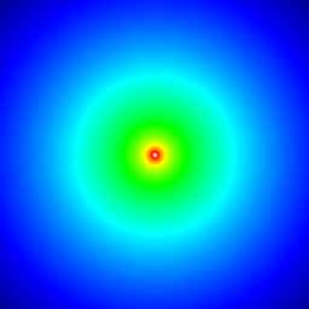
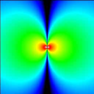
Figure 3: A slice through the center of the transfer functions in real space for the density field (left) and one component of the displacement field (right). The model parameters are the same as in Figure 2 except that a spherical Hanning filter (cosine in Fourier space) has been applied to reduce the anisotropy that was seen in Figure 2. False colors show the logarithm of the transfer function, with 6 orders of magnitude shown for the density and 3 orders of magnitude for the displacement. (The absolute value of the displacement is shown; it is negative in the right half of the image.) When convolved with white noise, these transfer functions give the density fluctuation and $x$-displacement fields in linear theory at redshift $z=0$.

The high-frequency part of the density field, $\delta_{1}=(\xi_{1}-\bar{\xi}_{1})\ast T$, is straightforward to calculate using the methods of §§2.3 and 2.4. Let us first consider the transfer functions for the density and displacement fields, which we show in Figure 3. In order to eliminate the anisotropy appearing in Figure 2, we have applied a spherical Hanning filter, multiplying $T(k)$ by $\cos(\pi k/2k_{\rm Ny})$ for $k<k_{\rm Ny}$ and zeroing it for $k>k_{\rm Ny}$ where $k_{\rm Ny}=\pi rM/L$. This filter has removed the anisotropic structure and has also smoothed the density field near $\vec{x}=0$. We have used the spherical method of §2.4.3. The exact method gives results that are visually almost indistinguishable, with maximum differences of order one percent because the Hanning filter does completely eliminate the anisotropy of the discrete Fourier transform.

Each Cartesian component of the displacement transfer function displays a characteristic dipole pattern because of the projection from radial motion: $\psi_{x}=(x/r)\psi(r)$. A density enhancement at the origin is accompanied by radial infall (with $\psi_{x}$ changing sign across the origin). Note that the displacement transfer function falls off much less rapidly with distance than the density transfer function, illustrating the well-known fact that the linear velocity field has much more large-scale coherence than the density field. The linear displacement, velocity, and gravity fields are all proportional to each other, so one may also interpret $\vec{T}_{\psi}$ as the transfer function for the gravitational field.

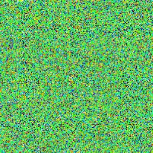
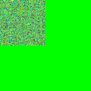
Figure 4: Slices through a sample of Gaussian noise in a cube of size 64 Mpc. Left: pure white noise $\xi_{1}(\vec{m},\vec{n}\,)$. Right: zero-padding is used for isolated boundary conditions, and the means have been subtracted over cells of size 1 Mpc so that we show $\xi_{1}(\vec{m},\vec{n}\,)-\bar{\xi}_{1}(\vec{m}\,)$. False colors are scaled to linear values ranging from $\pm 2$ standard deviations of $\xi_{1}$. The zero level is light green. Because of the predominance of high-frequency power, the filtering applied to the right-hand image is not apparent, but the two samples differ in the upper left quadrant.

The next step in computing the subgrid contribution to the initial conditions is to generate an appropriate sample of Gaussian noise. Figure 4 shows two samples of white noise for the high-resolution subgrid. The left sample is pure white noise $\xi_{1}(\vec{m},\vec{n}\,)$, which is the correct noise sample if we wish to generate a Gaussian random field with periodic boundary conditions on a grid of size 64 Mpc (the full width that is shown). The right sample is nonzero only in a region 32 Mpc across, as is appropriate for isolated boundary conditions in a subgrid, and the means over coarse grid cells have been subtracted, i.e. we plot $\xi_{1}(\vec{m},\vec{n}\,)-\bar{\xi}_{1}(\vec{m}\,)$. This is the appropriate noise sample for computing the short-wavelength density field $\delta_{1}$.

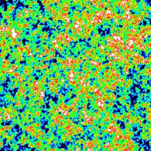
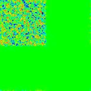
Figure 5: High resolution density fluctuation field obtained by convolving white noise (Figure 4) with the $\Lambda$CDM density transfer function (left panel of Figure 3). False colors are scaled to linear values ranging from $\pm 2$ standard deviations for the left panel. The left and right panels correspond to the same panels of Figure 4. The two density fields are strikingly different because long wavelengths have been suppressed in the right image by subtraction of coarse-cell means in Figure 4. The long wavelength components will be restored to the right image by addition of the coarse grid sample.

Figure 5 shows the result of convolving the two noise samples of Figure 4 with the density transfer function of Figure 3. The left-hand panel gives $\xi_{1}*T$ while the right-hand panel gives the desired short-wavelength field $\delta_{1}(\vec{m},\vec{n}\,)$. The two fields differ in the upper left quadrant because of the subtraction of coarse-cell means from the white noise field used to generate the left image. Although the effect of this subtraction is barely evident in Figure 4, it dominates the comparison of the two panels in Figure 5 because convolution by the transfer function acts as a low-pass filter. The left panel of Figure 5 gives a complete sample of $\delta(\vec{x}\,)$ on a periodic grid of size 64 Mpc, while the right panel shows only the short-wavelength components coming from mesh refinement.

Careful examination of the right panel of Figure 5 shows that the finite width of the transfer function has caused a little smearing at the boundaries, which are matched periodically to the opposite side of the box by the Fourier convolution. (A few pixels along the right and bottom edges of the left panel differ from green.) However, these edge effects do not represent errors in the short-wavelength density field. Instead, they illustrate the fact that outside of the refined region, the gravity field should include tidal contributions from the short-wavelength fluctuations inside the refinement volume. For the purpose of computing $\delta_{1}(\vec{m},\vec{n}\,)$ within the subvolume, we simply discard everything outside the upper left quadrant.

As a test of our transfer function methods, we calculated $\delta_{1}(\vec{m},\vec{n}\,)$ using the exact transfer function instead of the spherical one. The rms difference between the fields so computed was 0.0014 standard deviations, a negligible difference. As a test of the whole procedure, we computed the power spectrum of the left panel of Figure 5 and checked that it agrees within cosmic variance with the input $\Lambda$CDM power spectrum.

We also compared the displacement field computed using the exact transfer with that computed using the spherical one. The rms difference was 0.0062 standard deviations, still negligible. Then we compared the divergence of the displacement field (computed in Fourier space as $i\vec{k}\cdot\vec{\psi}$) with the density field, expecting them to agree perfectly. Interestingly, this is not the case for the exact (or spherical) transfer functions. When the transfer functions are truncated in real space and made periodic on a grid of size $(2M_{s}/M)L$, $T^{\prime}_{\delta}(\vec{k}^{\,\prime\,})\neq i\vec{k}^{\,\prime}\cdot\vec{T}^{\prime}_{\psi}(\vec{k}^{\,\prime\,})$ despite the fact that on the full refined grid $T_{\delta}(\vec{k}\,)=i\vec{k}\cdot\vec{T}_{\psi}(\vec{k}\,)$. The prime on the transfer functions indicates a different Fourier space, as discussed after equation (18). The only way to test $-\vec{\nabla}\cdot\vec{\psi}=\delta$ for the exact transfer function is to perform an FFT on the full refined grid of $(rM)^{3}=1024^{3}$ grid points. In §3.3 we will perform an equivalent test with an end-to-end test of the entire method using a $1024^{3}$ grid.

3.2 Long Wavelength Components

Now we consider $\tilde{\delta}_{0}(\vec{m},\vec{n}\,)$, the contribution to the density field from the coarse grid. As we see from equation (25), in principle we can compute $\tilde{\delta}_{0}$ by spreading the original coarse-grid white noise sample $\xi_{0}(\vec{m}\,)$ to the $r^{3}$ subgrid points for each coarse grid point (i.e., all $r^{3}M^{3}$ points) and then convolving with the high-resolution transfer function as in equation (16):

$$\tilde{\delta}_{0}(\vec{m},\vec{n}\,)=\sum_{\vec{m}^{\prime},\vec{n}^{\,\prime}}\xi_{0}(\vec{m}^{\,\prime})T(\vec{m}-\vec{m}^{\,\prime},\vec{n}-\vec{n}^{\,\prime})\ .$$ (26)

However, this method is impractical, because the contributions to $\tilde{\delta}_{0}$ coming from large distances are not negligible because of the long range of the transfer functions (especially for the velocity transfer function). For the short wavelength field $\delta_{1}(\vec{m},\vec{n}\,)$ this causes no problems because the noise field $\xi_{1}$ is nonzero only within the subvolume. Here, however, the noise field $\xi_{0}(\vec{m}\,)$ is nonzero over the entire simulation volume. Including all relevant contributions in the convolution as written would require working with the transfer function on the full grid of size $(rM)^{3}$, which is exactly what we are trying to avoid.

A practical solution is to rewrite equation (26) as a convolution of the coarse-grid density field with a short-ranged filter:

$$\tilde{\delta}_{0}(\vec{m},\vec{n}\,)=\sum_{\vec{m}^{\prime},\vec{n}^{\,\prime}}\delta_{0}(\vec{m}^{\,\prime})W(\vec{m}-\vec{m}^{\,\prime},\vec{n}-\vec{n}^{\,\prime})\ .$$ (27)

One can easily check that this is exactly equivalent to equation (26) provided that

$$W(\vec{m},\vec{n}\,)=(rM)^{-3}\sum_{\vec{k}}\exp[i\vec{k}\cdot\vec{x}(\vec{m},\vec{n}\,)]\,{T(k)\over T(k_{0})}$$ (28)

where $\vec{k}_{0}=(2\pi/L)\vec{\kappa}$ is the projection of $\vec{k}$ into the fundamental Brillouin zone (eq. 15).

An exact evaluation of equation (27) still requires using a full $(rM)^{3}$ grid. However, we will see that $W(\vec{x}\,)$ falls off sufficiently rapidly with distance that contributions to $\tilde{\delta}_{0}(\vec{m},\vec{n}\,)$ coming from large distances are negligible. (This will not be true for the velocity field, but we will develop a variation to handle that case later.) Thus, we may truncate $W(\vec{x}\,)$ at the boundary of the refinement region and perform the convolution of equation (27) using a $(2rM_{s})^{3}$ grid just as we did for the short-wavelength field. The errors of this procedure will be quantified below.

Equation (27) has a simple interpretation. The coarse-grid density field $\delta_{0}(\vec{m}\,)$ is spread to the fine grid by replicating the coarse-grid values to each of the $r^{3}$ grid points within a single coarse grid cell. The result is an artifact called aliasing. In real space this artifact is manifested by having constant values within pixels larger than the spatial resolution. In $k$-space the effect is to replicate low-frequency power in the fundamental Brillouin zone to higher frequencies. Thus, the wrong transfer function is used if one simply sets $\tilde{\delta}_{0}(\vec{m},\vec{n}\,)$ to $\delta_{0}(\vec{m}\,)$. Equation (28) defines an anti-aliasing filter which corrects the transfer function from the coarse grid (with wavevectors $\vec{k}_{0}$ in the fundamental Brillouin zone) to the full $k$-space. It smooths the sharp edges that arise from spreading $\delta_{0}(\vec{m}\,)$ to the fine grid. The anti-aliasing filter removes the artifacts caused by replication of the fundamental Brillouin zone.

The anti-aliasing filter is manifestly nonspherical, so we cannot use the spherical transform method of §2.4.3 to evaluate it. However, $W(\vec{m},\vec{n}\,)$ is sharply peaked. This is obvious from the fact that its Fourier transform is constant over the fundamental Brillouin zone; the Fourier transform of a constant is a delta function. Thus, we expect $W(\vec{m},\vec{n}\,)$ to be peaked on the scale of a few coarse grid spacings. As a result, the minimal $k$-space sampling method of §2.4.2 should suffice (with a variation for the velocity field).

The division by $T(k_{0})$ in equation (28) requires that we compute the coarse-grid density field $\delta_{0}(\vec{m}\,)$ without a Hanning filter; otherwise $T(k_{0})$ would be zero in the corners of each Brillouin zone. Simply put, if we want to correctly sample the density field at high resolution, we should not cut out long-wavelength power by filtering. However, we will apply a spherical Hanning filter at the shortest wavelength to remove the anisotropic structure that was apparent in Figure 2.

At the corners of each Brillouin zone $k_{0}=0$ but $k\neq 0$ (aside from the fundamental mode for the whole box). At these wavevectors, $\delta_{0}(\vec{m})$ has no power and so no error is made by setting $T(k)/T(k_{0})\to 0$. In the case of the displacement field, each component of $\vec{T}_{\psi}(\vec{k}_{0})$ vanishes along an entire face of the Brillouin zone, as explained in the paragraph before equation (23). We also set to zero these contributions to the Fourier series in equation (28).

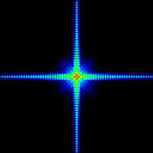
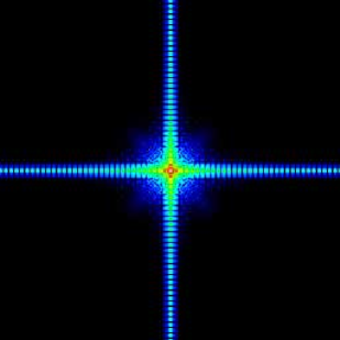
Figure 6: Anti-aliasing filter $W(\vec{m},\vec{n}\,)$ for the density. The left panel shows the filter computed using the exact method of §2.4.1 while the right panel uses the minimal $k$-space sampling method of §2.4.2. False colors are scaled to the logarithm of absolute value of the filter, which shows six orders of magnitude. The banded appearance is caused by low-amplitude oscillations. The oscillations act to smooth the sharp edges of the coarse grid fields when they are refined to the subgrid. The difference between the two filters is negligible away from the edges.

Figure 6 shows the density anti-aliasing filter computed with a spherical Hanning filter for $T(k)$. The minimal $k$-space method gives good agreement with the much slower exact calculation. Along the axes at the edges of the volume the errors are up to a factor of two, but $W$ is very small and oscillates, making these errors unimportant. The banding is due to the sign oscillations of $W$. They have a characteristic scale equal to the coarse grid spacing and they arise because of the discontinuity of $T(k)/T(k_{0})$ at Brillouin zone boundaries in equation (28). Such oscillations are characteristic of anti-aliasing filters. The filter falls off sufficiently rapidly with distance from the center that we can expect accurate results by truncating it outside the region shown.

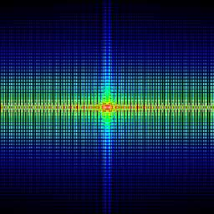
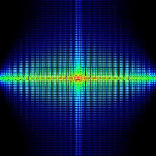
Figure 7: Anti-aliasing filters for the $x$-component of displacement (or velocity or gravity), computed with the exact (left) and minimal $k$-space sampling (right) methods. False colors are scaled to the logarithm of absolute value of the filter spanning four orders of magnitude. Because the displacement is sensitive to longer wavelengths than the density, the differences between the two computational methods here is more pronounced than for the density filter of Figure 6.

Figure 7 shows the corresponding result for the displacement (or velocity or gravity) field filter. (Recall that the displacement, velocity, and gravity are proportional to one another in linear theory.) Now the errors of the minimal $k$-space sampling method are significant. They arise because the minimal sampling method forces $W(\vec{m},\vec{n}\,)$ to be periodic on the scale of the box shown in the figure (twice the subgrid size) while with the exact method the scale of periodicity is larger by a factor $M/2M_{s}$ (or 4 in this case). In other words, the filter does not fall off very rapidly with distance, so truncating it and making it periodic in the box of size $2rM_{s}$ introduces noticeable errors. However, because the filter is still sharply peaked and oscillatory with small amplitude, it is possible that these errors are negligible. We will quantify the errors in §3.3.

The procedure is now similar to that of §3.1. Once we have the anti-aliasing filters, the next step is to obtain samples of the coarse-grid fields $\delta_{0}(\vec{m}\,)$ and $\vec{\psi}_{0}(\vec{m}\,)$ that we wish to refine. We do this using the convolution method of §2.1. For testing purposes, we construct a coarse-grid sample of white noise, $\xi_{0}(\vec{m}\,)$, which exactly equals the long-wavelength parts of the noise shown in the left panel of Figure 4. This was achieved by modifying GRAFIC (Bertschinger, 1995) to sample a white noise field $\xi(\vec{m}\,)$ in the spatial domain. Fourier transformation to $\xi(\vec{k}\,)$ then allows the calculation of density (and similarly displacement) by equation (7). As a result, we have chosen our coarse grid sample so that $\xi_{0}(\vec{m}\,)=\bar{\xi}_{1}(\vec{m}\,)$ within the refinement subgrid. This choice is made so that later we can see directly how long- and short-wavelength components of the noise contribute to the final density field.

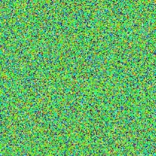
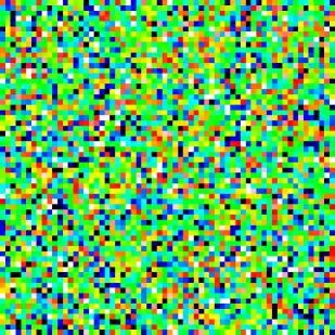
Figure 8: Slices through the white noise sample $\xi_{0}(\vec{m}\,)$ for the coarse grid. Left: Full cube of size 256 Mpc. Right: Magnification of the upper left corner by a factor of 4 to show the region that will be refined. Aliasing (sharp pixel boundaries) is now evident. False colors are scaled to linear values ranging from $\pm 2$ standard deviations.

Figure 8 shows the white noise sample adopted for the coarse grid. The right panel is obtained by averaging the left panel of Figure 4 over $4^{3}$ subgrid mesh points (1 Mpc³ volume). Figure 4 shows only a single thin slice of width 0.25 Mpc while Figure 8 shows coarse cells of thickness 1 Mpc, so one should not expect the two figures to appear similar. The left panel of Figure 8 shows a full slice of size 256 Mpc, obtained by filling out the rest of the volume with white noise.

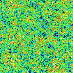
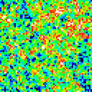
Figure 9: Slices through the coarse grid density field $\delta_{0}(\vec{m}\,)$ resulting from convolution of Figure 8 with the density transfer function sampled on the coarse grid. Left: Full cube of size 256 Mpc, with periodic boundary conditions. Right: Magnification of the upper left corner by a factor of 4 to show a square of size 64 Mpc. This panel shows the 32 Mpc region that we wish to refine to include the correct small-scale power. The magnified pixels represents an aliasing artifact. False colors are scaled as in Figure 5. Random numbers were chosen so that the right panel corresponds to the coarsely sampled long wavelength components of the left panel of Figure 5.

This white noise sample on the coarse grid was convolved with the transfer function using GRAFIC to give the coarse density field $\delta_{0}(\vec{m}\,)$ that we wish to refine. The results are shown in Figure 9. The right panel shows a 64 Mpc subvolume including the 32 Mpc refinement region. The obvious pixelization is the result of mesh refinement: the coarse grid density field has been spread to the fine grid. This pixelization causes power from wavelengths longer than the coarse grid spacing to be aliased to higher frequencies. If uncorrected, this aliasing would introduce spurious features into the power spectrum. Thus, the coarse grid sample must be convolved with an anti-aliasing filter as described above.

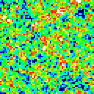
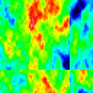
Figure 10: Slices through the density (left) and velocity (x-component, right) fields on the coarse grid after a buffer region of width 16 Mpc has been placed around the 32 Mpc subvolume in the upper left. In the upper left 48 Mpc area, the left panel matches the right panel of Figure 9. The bottom and right quartiles are filled with values from the top and left of the subvolume which were then wrapped periodically. This is clearer for the velocity field because of its larger coherence length. The buffer regions and periodic boundary conditions are needed because of the FFT-based method for convolution with anti-aliasing filters.

Special care is needed with the boundary conditions for the anti-aliasing convolution of equation (27). The top grid density field $\delta_{0}(\vec{m}\,)$ fills the subgrid shown in the right panel of Figure 9 without periodic boundary conditions. The anti-aliasing filter (Fig. 6) has finite extent; therefore FFT-based convolution of the two will lead to spurious contributions to $\tilde{\delta}_{0}$ at the subvolume edges coming from $\delta_{0}$ on the opposite side of the box. To avoid this, we surround the subvolume (which occupies one octant of the convolution volume) with a buffer region of width one-half of the subvolume in each dimension. The correct density values from the top grid are placed in this buffer. Because our subvolume is not centered but rather is placed in the corner of the cube of size $2rM_{s}$, we wrap half of the buffer to the other side of this cube. The results are shown in Figure 10.

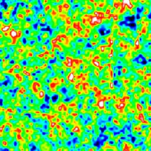
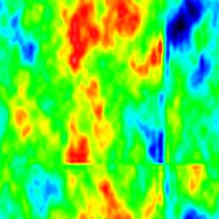
Figure 11: Long-wavelength density and velocity fields after convolution by the anti-aliasing filter. Each panel is the convolution of the corresponding panel of Figure 10 by the appropriate anti-aliasing filter (Fig. 6 for the density, Fig. 7 for the velocity). The anti-aliasing filters have eliminated the pixelization artifacts present in Figure 10. Convolution across the discontinuity at the boundary of the buffer region causes some errors but these are small within the desired refinement region (the upper left quadrant in these images).

Figure 11 shows the density field $\tilde{\delta}_{0}(\vec{m},\vec{n}\,)$ and the corresponding velocity field after convolution with the anti-aliasing filter $W$. The minimal $k$-space filter has been used here; there would be almost no discernible difference if the exact filter was used instead. The pixelated images of Figure 10 have now been smoothed appropriately for the transfer function. Smoothing over pixelization artifacts is the purpose behind anti-aliasing filters, whether they be applied in image processing or cosmology.

The convolution method used here is not exact. Quantifying its errors requires evaluating equation (26) or (27) using a full convolution of size $(rM)^{3}$. We do this in the next subsection, where we test all stages of the mesh refinement method.

3.3 Testing the Refined Fields

Having computed separately the short- and long-wavelength contributions to the density and velocity (or displacement) fields, we combine them in Figure 12 using equation (24) to give the complete multiscale fields. The four-fold increase in resolution can be seen by comparing the subvolume with the rest of the field. The effects of higher resolution are much more pronounced for the density than they are for the velocity because of the density field’s steeper dependence on wavenumber.

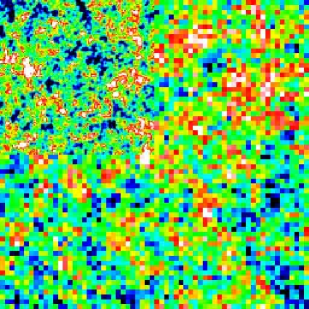
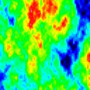
Figure 12: Slices through the 2-level linear density (left) and velocity (right, $x$-component) fields in a region 64 Mpc across extracted from the 256 Mpc realization. False colors are scaled to linear values ranging from $\pm 2$ standard deviations of the high-resolution fields. The refinement subgrid is the upper left quadrant in each case. Outside of this region the coarse (top) grid values are shown to illustrate how mesh refinement increases the resolution. The density figure may be compared directly with the right-hand panel of Figure 9.

A test of the entire mesh refinement procedure can be made by generating the density and velocity fields at full $1024^{3}$ resolution over the whole 256 Mpc box. This was done by modifying the author’s GRAFIC code (Bertschinger, 1995) to replace its random numbers in $k$-space with an input white noise field in real space. The noise field was constructed to match the upper left quadrant of the left panel of Figure 4 in a high-resolution region 32 Mpc across and to match the left panel of Figure 8 everywhere else, with noise values made uniform in 1 Mpc cells ($4^{3}$ grid cells of the $1024^{3}$ grid). Thus, the white noise field was sampled as in Figure 1. In order to have sufficient computer memory, GRAFIC was run on the Origin 2000 supercomputer at the National Computational Science Alliance.

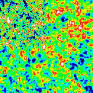
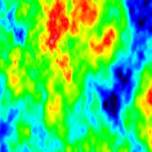
Figure 13: Density (left) and velocity (right) fields computed using a full $1024^{3}$ grid with random numbers chosen to match the multiscale calculation. This figure gives the exact results against which to compare Figure 12.

The results of this full-resolution calculation are shown in Figure 13. The high-resolution fields are smooth outside of the refinement volume simply because they have been convolved with a high-resolution transfer function; by contrast, Figure 12 shows only the sampling of a low-resolution mesh outside of the subvolume. These resolution differences are not important here. Rather, it is the comparison in the high-resolution subvolume that is important. Evidently the density field is accurately reproduced by the multiscale algorithm while there are some visible errors in the velocity field.

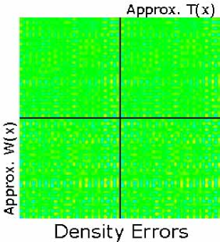
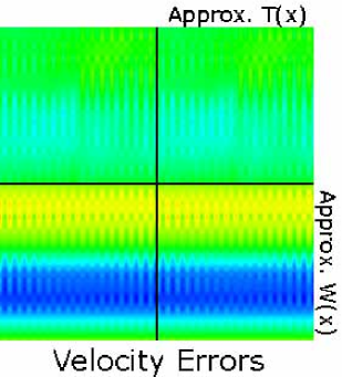
Figure 14: Errors in the mesh-refined density and velocity fields obtained by subtracting the upper left quadrants of Figures 12 and 13. False colors are scaled to $\pm 0.005$ standard deviations for the density errors and $\pm 0.2$ standard deviations for the velocity errors. Each map is a mosaic of 4 panels showing the errors resulting from the two major approximations used in the multiscale computation. The right columns, labelled “Approx. T(x),” show the effect of the spherical transform method for computing the transfer functions. The lower rows, labelled “Approx. W(x),” show the effect of the minimal $k$-space sampling method for computing the anti-aliasing filters. The upper-left quadrants show the errors when exact (and computationally expensive) transfer and anti-aliasing filters are used while the lower-right quadrants show the errors in Figure 12. There are residual errors even with exact $T(\vec{x}\,)$ and $W(\vec{x}\,)$ because of the spatial truncation of $W$.

To quantify these errors, in Figure 14 we show residuals obtained by subtracting the exact maps from the multiscale maps for the 32 Mpc refinement subvolume. A priori we expect three main sources of error:

1. The use of the spherical method for fast computation of the short-wavelength transfer functions;

2. The use of the minimal $k$-space sampling method for fast computation of the long-wavelength anti-aliasing filters; and

3. Truncation of the anti-aliasing filter to perform the convolution over a subvolume instead of the entire top grid.

All three effects are visible in Figure 14. The rows and columns that are not labeled use the exact filters but are still subject to the third error, truncation of $W(\vec{x}\,)$.

Scaled to the standard deviation of the high-resolution density field, the rms errors of density in the subvolume shown in Figure 14 are 0.04% (upper left), 0.09% (upper right), 0.06% (lower left), and 0.10% (lower right). Thus, the major source of error for adaptive refinement of the density field is the use of a spherical transfer function for the short-wavelength components. The magnitude of the error is insignificant for the accuracy of cosmological simulations. For the velocity field, on the other hand, the corresponding rms errors are 3.2% (top row) and 7.0% (bottom row). Clearly the anti-aliasing filter step is causing problems for the long-wavelength velocity field.

3.4 Solving the Anti-aliasing Problems for the Velocity Field

The long-range coherence of the velocity (or gravity) field has been seen to cause difficulties for the evaluation of the long-wavelength components by anti-aliasing the coarse-grid sample. This subsection presents a solution.

Several attempts were made to reduce the anti-aliasing errors while continuing to use a minimal $k$-space sampling algorithm. None of the attempts succeeded until we split the long-wavelength velocity field from the top grid into parts due separately to the mass inside and outside the refinement subvolume. The motivation for this was the idea that the latter part (the tidal field within the subvolume caused by mass outside it) might be smooth enough to require minimal interpolation to the subgrid. For convenience, tidal split was done by setting $\xi_{0}(\vec{m}\,)=0$ outside or inside the subvolume instead of setting $\delta_{0}(\vec{m}\,)=0$; the coherence length of the density field is so small that very little difference is made either way. Linearity of the velocity field ensures that when we add together the two parts either way we get the complete long-range velocity field.

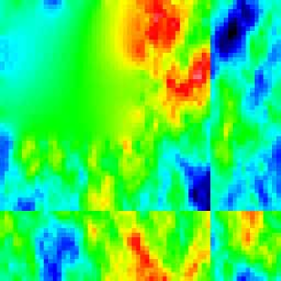
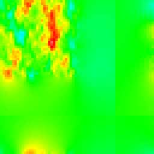
Figure 15: Split of the coarse-grid velocity field into parts due to fluctuations outside (left, “outer part”) and inside (right, “inner part”) of the refinement subvolume. The two maps together add to give the velocity map of Figure 10. This decomposition is the key to reducing the anti-aliasing velocity field errors, as described in the text.

Figure 15 shows the decomposition of the velocity field into the “outer” and “inner” parts. They were computed by zeroing the white noise field in the appropriate regions and re-running GRAFIC. The same boundary conditions are used as in Figure 10. The character of the two parts is strikingly different within the refinement subvolume (the upper left quadrant). The outer part is smooth, as expected. The inner part has a smaller coherence length and it is well-localized over the upper left quadrant. This spatial localization and coherence suggest that the truncated minimal $k$-space filter will be much more accurate for the inner part than for the complete velocity field. For the outer part, on the other hand, we know that the discontinuities at the boundary of the buffer regions will cause appreciable errors if convolved with the same filter. The smoothness of the tidal field inside the subvolume suggests that we use a much simpler and more localized filter.

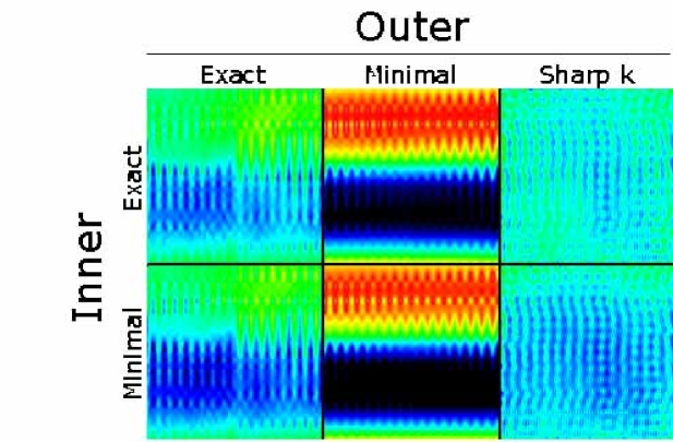
Figure 16: Velocity field errors under different approximations for evaluation of the inner and outer parts shown in Figure 15. The false colors are scaled to $\sigma/10$ where $\sigma$ is the standard deviation. The upper left (exact/exact) and lower middle (minimal/minimal) maps are the same as the two rightmost maps in Figure 14, where they were imaged with a color stretch only half as large ($\sigma/5)$. RMS errors for each map (as a percentage of the rms one-dimensional velocity) are 3.2, 6.8, 2.7 (top row, left to right) and 3.6, 7.0, 3.2 (bottom row). The bottom right map gives the errors for the best fast method. As in Figure 14, there are errors even in the “exact” case because of the truncation of the anti-aliasing filter.

Several different filters were tried for the outer (tidal) part of the velocity field. The results for three are shown in Figure 16. The best simple filter was found to be sharp $k$-space filtering, which sets $W(\vec{k})=0$ everywhere except the fundamental Brillouin zone, where $W(\vec{k}\,)=1$ (before the Hanning filter applied at the fine mesh scale). This filter completely eliminates the aliasing error by eliminating the replication of the fundamental Brillouin zone in $k$-space. It is also much more localized than the exact filter, so that spurious effects from the buffer truncation in the left panel of Figure 15 are not convolved into the subvolume. The price one pays is that it has the wrong shape at small distances compared with the exact filter, leading to a new source of errors in the rightmost columns of Figure 16. However, these errors are smaller than the error made with the exact filter due to the buffer truncation (top left panel).

A comparison of the top and bottom rows of Figure 16 shows that the filtering of the inner part of the velocity field is a minor source of error. It is the tidal field (the outer part) that requires delicate handling. Using a sharp $k$-space filter for the outer part and minimal $k$-space filter for the inner part, our final errors are 3.2% rms, the same as if we had used the computationally expensive exact filter throughout. These errors are probably small enough to be unimportant in cosmological simulations. They could be further reduced, at the expense of an increase in computer time and memory, by increasing the size of the buffer region for the top grid.

4 MULTIPLE REFINEMENT LEVELS

The ability to refine an existing mesh opens the possibility of recursive refinement to multiple levels, offering a kind of telescopic zoom into cosmic structures. Before this digital zoom lens can work, however, there are some implementation issues to face. The issues addressed in §3.3 must be considered anew in light of recursive refinement.

To see the issues arising in recursive refinement, consider a three-level refinement with refinement factors $r_{1}$ and $r_{2}$. By analogy with equations (10) and (12), we write the grid coordinates and noise fields as

$$\vec{x}(\vec{m},\vec{n},\vec{o}\,)=\vec{x}_{o}+\left(L\over M\right)\left(\vec{m}+{1\over r_{1}}\vec{n}+{1\over r_{1}r_{2}}\vec{o}\,\right)\ .$$ (29)

$$\xi(\vec{m},\vec{n},\vec{o}\,)=\xi_{2}(\vec{m},\vec{n},\vec{o}\,)+\xi_{1}(\vec{m},\vec{n}\,)-\bar{\xi}_{2}(\vec{m},\vec{n}\,)+\xi_{0}(\vec{m}\,)-\bar{\xi}_{1}(\vec{m}\,)$$ (30)

where $\bar{\xi}_{2}$ is obtained by averaging $\bar{\xi}_{2}$ over $\vec{o}$. At each level of the hierarchy there is a different grid (labeled by $\vec{m}$, $\vec{n}$, and $\vec{o}$, respectively). The variances of the white noise samples are related by ${\rm Var}(\xi_{2})=r_{2}^{2}{\rm Var}(\xi_{1})=r_{1}^{2}r_{2}^{2}{\rm Var}(\xi_{0})$.

The main idea of recursive refinement is that, once we have refined to level $n$ (where $n=0$ is the periodic top grid before any refinement), the fields computed at that level serve as top-grid fields to be refined to level $n+1$. Equations (24), (25), and (27) showed how that refinement works for $n=0$ by applying an anti-aliasing filter to the level-0 fields. For $n=1$ we get

$$\delta(\vec{m},\vec{n},\vec{o}\,)=\delta(\vec{m},\vec{n}\,)\ast W+\left[\xi_{2}(\vec{m},\vec{n},\vec{o}\,)-\bar{\xi}_{2}(\vec{m},\vec{n}\,)\right]*T\ .$$ (31)

The procedure for refinement to an arbitrary level is now clear. First we sample the fields at the preceding level and spread them to the new fine grid. Then we convolve with the appropriate anti-aliasing filter. Next we sample short-wavelength noise on the new fine grid and subtract the coarse-cell means so that so that the noise is zero at every higher level of the hierarchy. This noise is then convolved with the transfer function and added to the long wavelength field to give the high-resolution field. This procedure is the same for all levels of the hierarchy. However, there are some issues to consider involving the transfer functions and anti-aliasing filters. We discuss these next.

4.1 Short Wavelength Components

As was the case for two-level refinement, exact sampling requires that we compute the upper-level sample without any filtering. That is, we should eliminate the Hanning filter from both the anti-aliasing filter $W$ and the transfer function $T$ before computing all refinements except the last one at the highest degree of refinement. Otherwise we would lose power present in the intermediate refinement levels.

Eliminating the Hanning filter is straightforward for the anti-aliasing filters used in §3. The minimal $k$-space and sharp $k$-space filters are equally easy to compute with or without a Hanning filter. However, the transfer functions are an altogether different matter. In §3.1 we used spherical transfer functions after concluding in §2.4.2 that the coarse $k$-space sampling of the minimal method would give significant errors for the short-wavelength fields.

Unfortunately, the unfiltered density transfer function is anisotropic, as was shown in Figure 2. It also has a higher peak value than the filtered transfer function in Figure 3. Computing the exact transfer function is unacceptably costly, with the operations count scaling as the sixth power of the total refinement factor (i.e. the product of the individual refinement factors for each level). Thus, we are forced to reconsider the spherical and minimal sampling methods for the transfer functions.

The unfiltered density is nonspherical because $k$-space is sampled in a cube instead of a sphere. Besides creating anisotropy, this sampling increases the small-scale power. As an alternative, we might use the spherical method of equation (22) with a Hanning filter but with a maximum spatial frequency (i.e. the cutoff for the Hanning filter) larger than the Nyquist frequency $\pi/\Delta x$ for grid spacing $\Delta x$. This is easily done by increasing the Nyquist frequency by a factor $f>1$ to include the high-frequency waves in the Brillouin zone corners with $|\vec{k}|>\pi/\Delta x$. For $f=1.838$ and the power spectrum parameters used before, this method reproduces the correct peak value of the density transfer function. However, the spherical method cannot reproduce the anisotropy evident in Figure 2, which is important on small scales. (For multilevel refinement, exact sampling requires that we use the anisotropic transfer functions at all but the finest refinement. The refinement process itself magnifies cubical pixels. This anisotropy is cancelled by summing over the contributions from different levels of the hierarchy only if we use anisotropic filters.) On the other hand, the velocity transfer function is an integral over the density transfer function and therefore is much smoother. Errors at small $r$ due to the neglect of anisotropy are much less important for the velocity field. Thus, we might approximate the correct, anisotropic transfer function for the radial velocity by the spherical one.

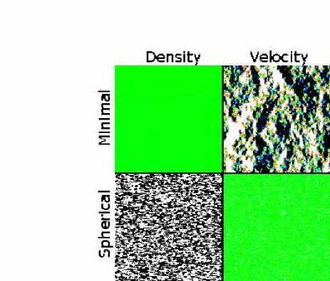
Figure 17: Errors of the short-wavelength density (left) and velocity (right) fields computed without a Hanning filter, using spherical and minimal $k$-space filters as described in the text. The density errors have been scaled to $\sigma/200$ and the velocity errors to $\sigma/10$. The minimal method is accurate at small spatial scales (density) while the spherical method is accurate at large scales (velocity).

Based on these considerations, we reconsider both the spherical and minimal $k$-space sampling methods for approximating the unfiltered transfer functions. Figure 17 shows the residuals from the exact, anisotropic transfer functions. Comparison with Figure 14 shows that removal of the Hanning filter adds no significant errors provided that the minimal method is used for the density and the spherical method is used for the velocity. The spherical method works poorly for the density field because it neglects the small-scale anisotropy. The minimal method works poorly for the velocity field because it assumes periodicity on a scale twice the subgrid extent.

The minimal sampling method works better than expected for the density transfer function. The reason for its success is that for CDM-like power spectra the transfer function is dominated by large spatial frequencies for which the coarse sampling of Fourier space introduces little error in the discrete Fourier transform. For the velocity transfer function, long-wavelength contributions dominate and the small-scale errors of the spherical method cause little harm.

4.2 Long Wavelength Components

The next issue to consider is the treatment of tidal fields from coarser levels of the grid hierarchy during the anti-aliasing step. As we found in §3.4, contributions from fluctuations inside the subvolume can be filtered using the minimal $k$-space sampling method, but contributions from tides generated outside the subvolume must be convolved with a sharp $k$-space filter. This requires a clear separation of “inner” and “outer.” Care is needed in the case of a multilevel hierarchy.

Consider, for example, refinement of the 256 Mpc top grid shown in Figure 9 in two stages to produce the four-fold refinement of the 32 Mpc level-2 subvolume in Figure 12. The level-1 subvolume may have any size between 64 and 128 Mpc. (Each refinement must be over a subvolume no more than half the size of the upper-level volume in order to accomodate the buffer region used in the anti-aliasing step.) When computing the long-wavelength velocity contributions for the level-2 grid, the level-1 fields must be computed with a tidal volume of 32 Mpc and not the size of the level-1 subvolume. Moreover, the same is true of the level-0 fields. Correct treatment of the tidal fields requires that all upper levels be sampled with $\xi=0$ inside (or outside) the final high-resolution subvolume.

This requirement implies that a chain of refinements must be performed for every level of the hierarchy. Computing a level-1 refinement requires only one application of convolution plus small-scale noise. Computing a level-2 refinement requires two applications: one to get the level-1 samples with the correct tidal volume and a second to get the level-2 results. Thus, computing all three levels (0, 1, and 2) requires three runs of the periodic grid routine in a box of size 256 Mpc (with no tides, with tides for the level-1 subvolume, and with tides for the level-2 subvolume) plus three runs of the refinement algorithm.

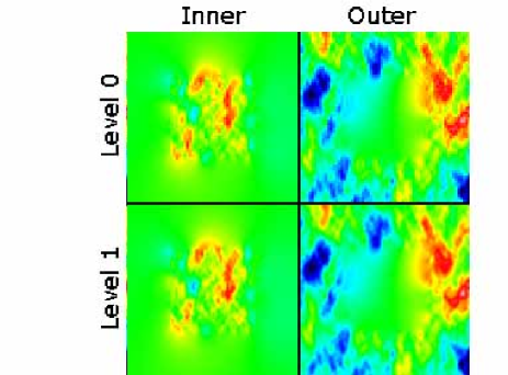
Figure 18: Tidal fields in a volume 64 Mpc across from level 0 (top) and after refinement to level 1 (bottom). This figure shows the successive refinement of the tidal fields needed for computation of the level-2 velocity field. The anti-aliasing has been performed without a Hanning filter in order to preserve exact sampling of the power spectrum.

The process of successive refinement is illustrated in Figure 18 for the computation of the level-2 velocity field. The top row is the same as Figure 15 except that the buffer has been unwrapped to surround the volume. However, instead of being prepared for a $r=4$ refinement, these top-level fields are prepared here for a $r=2$ refinement. They are convolved with the appropriate anti-aliasing filters and short wavelength noise is added to give level 1, shown in the lower row. The level-1 tidal fields are resolved better and do not suffer from aliasing at the resolution shown (0.5 Mpc grid spacing). These fields provide the input to a final $r=2$ refinement to produce the level-2 fields.

Comparing the resulting level-2 fields with Figure 13, we find that the magnitude of the errors depends on the size of the level-1 grid. For the case shown in Figure 18, with a 64 Mpc grid, the rms density and velocity errors are 0.02% and 3.9%, respectively. When the level-1 grid size is increased to its maximum value of 128 Mpc, these errors drop to 0.0094% and 3.3%, respectively. These compare with the errors for a single $r=4$ refinement, 0.10% and 3.2%, respectively.

The density errors have decreased with two $r=2$ refinements compared with one $r=4$ refinement mainly because the minimal $k$-space sampling of the anti-aliasing filter is coarser (hence less accurate) for $r=4$. For the velocity field the errors are dominated not by the coarse sampling errors in $W(\vec{x}\,)$ but rather in the errors due to its truncation. In other words, it is the discontinuities at the edge of the buffer region (shown in Figure 15) that cause problems. However, when the top grid is refined by $r=2$ in a subvolume of half its size, the doubling used for the convolution has a fortunate side effect: the buffer region fills out the volume so that the entire top grid is included. In this special case, which applies to our 128 Mpc level-1 grid, there are no errors from periodic boundary conditions and the minimal $k$-space filter is exact. The errors arise almost exclusively from the second level of refinement. Thus, the two-level refinement in this case has the same velocity field errors as a single $r=4$ refinement.

5 MORE TRICKS WITH CONVOLUTION OF WHITE NOISE

The convolution method presented in this paper lends itself to a variety of tricks that can be done with sampling of Gaussian random noise. These need not always involve adaptive mesh refinement and convolution with isolated boundary conditions. For example, in Figure 13 we achieved multiscale initial conditions using a single high-resolution grid but with the white noise sampled more finely within a subvolume. This procedure has the advantage of allowing multiscale fields to be computed free from aliasing errors. Although it is limited by computer memory constraints, this method is the preferred choice for producing multiscale fields when computer memory is not a limitation.

Our white noise sampling and convolution methods offer another way to change the dynamic range of a simulation while retaining the sampling of a fixed set of cosmic structures. Instead of refining to small scales, one may change the large scale structure in the simulation by expanding or shrinking the top grid size. This offers a simple and useful way, for example, to add or subtract long waves in order to examine their effect on small scale structure. This brief section presents the method for expanding or shrinking a simulation.

One way to implement this idea, which we will not explore further, is to take an existing small-scale simulation to provide the high-resolution field $\delta_{1}(\vec{m},\vec{n}\,)$ as in equation (24). The small volume, originally with periodic boundary conditions, is then embedded with isolated boundary conditions in a new top grid field $\delta_{0}(\vec{m}\,)$. The white noise sample used to generate the existing small-scale simulation is taken to be $\xi_{1}(\vec{m},\vec{n}\,)$ and a new sample is created for the top grid. This procedure is the same as that described in §3 except that there the top grid sample was given and the subgrid sample was added. Here it is the other way around. The implementation proceeds as in §3. It is straightforward and need not be elaborated.

An alternative method is to change the size of an existing grid while retaining a fixed grid spacing without refinement. This method is easy to implement because no aliasing occurs if the grid is not refined. Moreover, periodic boundary conditions are used for all convolutions. We simply change the scale of periodicity. This can be achieved using a modified version of the GRAFIC code (Bertschinger, 1995) called GRAFIC1 which is being distributed along with the mesh-refinement version GRAFIC2.

The procedure is as follows. First, identify a volume (perhaps a subvolume of an existing simulation) whose size is to be changed. GRAFIC1 should be run so as to output the white noise field $\xi(\vec{m}\,)$ used in constructing the initial conditions. Note that the spatial mean noise level $\bar{\xi}$ vanishes so that the mean density matches that of the background cosmological model. This is a consequence of periodic boundary conditions.

The white noise field is now expanded with the addition of new white noise if one wishes to expand the box. If one wishes to shrink the box instead, then some of the noise field is excised. The amplitude of the white noise must be changed according to equation (9). For example, if the grid size is doubled in each dimension, the existing sample must be multiplied by $2^{3/2}$ and the added noise must have the same variance. These manipulations are easy to perform in real space. The absence of any correlations for the white noise makes the treatment of boundary conditions very simple. Note that $\bar{\xi}$ must vanish on the final grid because of periodic boundary conditions. However, if the volume has been expanded by a factor $f>1$, the mean value within the original volume can be changed by adding a constant, e.g. a normal deviate with variance $f$.

Finally, the new white noise field is now given as input to a second run of GRAFIC1, which calculates the density and velocity fields using exact transfer functions.

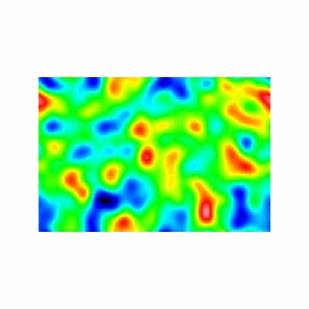
Figure 19: Slices of the density field from a realization of the Hot Dark Matter model. Left: a cube of size 512 Mpc. Right: a parallelpiped of dimensions $384\times 256\times 400$ Mpc has been extracted to create a new volume with periodic boundary conditions and with the same structures as the sample on the left.

This procedure is illustrated in Figure 19. One sees that the structures in the left original volume are reproduced in the new sample but that they are modified at the edges by the requirement of periodic boundary conditions. This affects the structure to within a distance of a few coherence lengths. The Hot Dark Matter model (with $\Omega_{m}=1$ and $h=0.5$) was chosen for this test so that the coherence length would be interestingly large. One also sees that the initial conditions codes do not require the volume to be a cube nor the axis lengths to be powers of 2. GRAFIC1 and GRAFIC2 allow for arbitrary parallelpipeds as long as there is at least one factor of two in each axis length.

6 CONCLUSIONS AND CODE DISTRIBUTION

We have presented an algorithm for adaptive mesh refinement of Gaussian random fields. The algorithm provides appropriate initial conditions for multiscale cosmological simulations. Aside from small numerical errors, the density and velocity fields at each refinement level are exact samples of Gaussian random fields with the correct correlation functions including all contributions from tides generated at lower-resolution refinement levels. An arbitrary number of refinement levels is allowed in principle, enabling cosmological simulations to be performed which have the correct sampling of fluctuations over arbitrarily large dynamic ranges of length and mass.

Two convolutions are performed per refinement level for each field component. These convolutions are performed using FFTs with the grid doubled in each dimension. Thus, the computer memory and time requirements for adaptive mesh refinement are significantly greater than for sampling of Gaussian random fields with a single grid. One advantage of the refinement algorithm is that the dynamic range in mass is not limited by the size of the largest FFT that can fit into memory. Also, it automatically provides the correct initial conditions for multiscale simulations such as that of Abel et al. (2000).

Adaptive mesh refinement of Gaussian random fields is more complicated than refinement of, for instance, the fluid variables in a hydrodynamics solver. The reason for this is that Gaussian random fields have long-range correlations. Correct refinement within a subvolume cannot be done independently of the lower resolution fields outside that subvolume. When the resolution is increased by decreasing the pixel size, a given sample suffers from aliasing. Correct sampling requires convolution by an anti-aliasing filter. Short-wavelength contributions are then provided by convolution of white noise with the appropriate transfer function.

Due mainly to imperfect anti-aliasing, numerical errors prevent one from achieving perfect sampling of multiscale initial conditions. However, with careful analysis of the source of errors — primarily from tides generated outside the subvolume — we have reduced these errors to an acceptable level. In testing with a realistic cosmological model, the rms errors for a four-fold refinement were 0.1% or smaller for the density and 3% for the velocity. We showed that the most accurate results are achieved by refinement factors of two, with each successive subvolume occupying one-eighth the volume (half the linear extent) of the parent mesh. For a single refinement level, the anti-aliasing errors vanish in this case.

Further testing is advised before the code is run to more than 4 refinement levels or a total refinement greater than 16. Also, some of the same numerical issues (e.g. refinement of tidal fields) identified here may arise in the gravity solvers used by nonlinear evolution codes. Careful testing of both the initial conditions and the nonlinear simulations codes is advised before workers apply them to dynamic ranges in mass exceeding $10^{11}$. Unfortunately, it is very difficult to provide exact standards for comparison with grid hierarchies of such large dynamic range.

The algorithm described in this paper has been implemented in FORTRAN-77 and released in a publically available code package that can be downloaded from http://arcturus.mit.edu/grafic/. The package has three main codes:

1. LINGERS is an accurate linear general relativity solver that calculates transfer functions at a range of redshifts.

2. GRAFIC1 computes single-grid Gaussian random field samples with periodic boundary conditions.

3. GRAFIC2 refines Gaussian random fields starting with those produced by GRAFIC1. It may be run repeatedly to recursively refine Gaussian random fields to arbitrary refinement levels.

LINGERS is a modification of the linger_syn code from the COSMICS package (Bertschinger, 1995; Ma & Bertschinger, 1995). It produces output at a range of times enabling accurate interpolation to the starting redshift of the nonlinear cosmological simulation. CMBFAST (Seljak & Zaldarriaga, 1996) could be used instead, although the treatments of normalization and units are different for the two codes.

GRAFIC1 is a modification of the grafic code from COSMICS that incorporates exact transfer functions for both CDM and baryons at arbitrary redshift from LINGERS and uses white noise sampled in real space as the starting point for Gaussian random fields. As demonstrated in §5, sampling of white noise enables one to change the size of the computational volume, or to embed a given realization into a larger volume with different resolution, simply by modifying the noise file. GRAFIC1 and GRAFIC2 also have optional half-mesh cell offsets for the CDM or baryon grids.

GRAFIC2 is the multiscale adaptive mesh refinement code. It requires substantial computing requirements for large grids, mainly because of the need to double the extent of each dimension. Thus, suppose that one has a $256^{3}$ top grid and wishes to double the resolution in one-eighth of the volume. Computing the $256^{3}$ sample with GRAFIC1 requires 64 MB of memory. Refining it with GRAFIC2 requires 1.02 GB of memory and 3.5 GB of scratch disk. The cpu time is also much larger, but is still far less than the time required for the nonlinear evolution. Fortunately, these computing resources are now available on desktop machines. Much larger grids are possible with parallel supercomputers.

I thank my colleagues in the Grand Challenge Cosmology Consortium — J. P. Ostriker, M. L. Norman, and L. Hernquist — for encouragement in this work. Special thanks are given to L. Hernquist and the Harvard-Smithsonian Center for Astrophysics for hosting my sabbatical during this work. Supercomputer time was provided by the National Computational Science Alliance at the University of Illinois at Urbana-Champaign. Financial support was provided by NSF grants ACI-9619019 and AST-9803137.

References

- Abel et al. (2000) Abel, T., Bryan, G. L., & Norman, M. L. 2000, ApJ, 540, 39
- Bertschinger (1995) Bertschinger, E. 1995, COSMICS software release (astro-ph/9506070)
- Bertschinger (1998) Bertschinger, E. 1998, ARA&A, 36, 599
- Colberg et al. (2000) Colberg, J. M. et al., MNRAS, 319, 209
- Fukushige & Makino (1997) Fukushige, T. & Makino, J. 1997, ApJ, 477, L9
- Ghigna et al. (2000) Ghigna, S., Moore, B., Governato, F., Lake, G., Quinn, T., & Stadel, J. 2000, ApJ, 544, 616
- Hoffman & Ribak (1991) Hoffman, Y. & Ribak, E. 1991, ApJ, 380, L5
- Katz et al. (1994) Katz, N., Quinn, T., Bertschinger, E., & Gelb, J. 1994, MNRAS, 270, L1
- Ma & Bertschinger (1995) Ma, C.-P. & Bertschinger, E. 1995, ApJ, 455, 7
- Pen (1997) Pen, U.-L. 1997, ApJ, 490, L127
- Salmon (1996) Salmon, J. 1996, ApJ, 460, 59
- Seljak & Zaldarriaga (1996) Seljak, U. & Zaldarriaga, M. 1996, ApJ, 469, 437