A New Method for ISOCAM Data Reduction – I. Application to the European Large Area ISO Survey Southern Field: Method and Results

Abstract

We have developed a new data reduction technique for ISOCAM LW data and have applied it to the European Large Area ISO Survey (ELAIS) LW3 (15 $\mu$m) observations in the southern hemisphere (S1). This method, known as LARI technique and based on the assumption of the existence of two different time scales in ISOCAM transients (accounting either for fast or slow detector response), was particularly designed for the detection of faint sources. In the ELAIS S1 field we obtained a catalogue of 462 15 $\mu$m sources with signal-to-noise ratio $\geq$ 5 and flux densities in the range $0.45-150$ mJy (filling the whole flux range between the Deep ISOCAM Surveys and the IRAS Faint Source Survey). The completeness at different flux levels and the photometric accuracy of this catalogue have been tested with simulations. Here we present a detailed description of the method and discuss the results obtained by its application to the S1 LW3 data.

1 Introduction

The Infrared Space Observatory (ISO; Kessler et al. 1996) was the successor to the Infrared Astronomical Satellite (IRAS). ISO, besides carrying out detailed studies of individual objects and small regions, has provided an opportunity to perform survey work at sensitivities of several orders of magnitude better than its precursor. Thus, a significant fraction of the mission time was spent on field surveys. The largest survey conducted with ISO is the European Large Area ISO Survey (ELAIS), which provides a link between the IRAS survey and the deeper ISO surveys. ELAIS is a collaboration between 20 European institutes which involves a deep, wide-angle survey at high Galactic latitudes, at wavelengths of 6.7 $\mu$m, 15 $\mu$m, 90 $\mu$m and 175 $\mu$m with ISO (see Oliver et al. 1997 and Oliver et al. 2000 for a detailed description of the Survey). In particular, the 15 $\mu$m survey was carried out with the ISO-CAM camera (Cesarsky et al. 1996) over a total area of $\sim$ 13 deg², divided into 4 main fields and several smaller areas. One of the main fields, S1, and one of the smaller areas, S2, are located in the southern hemisphere. S1 is centered at $\alpha$(2000) = 00^h 34^m 44.4^s, $\delta$(2000) = -43^∘ 28^′ 12^′′ and covers an area of $2^{\circ}\times 2^{\circ}$, while S2 is centered at $\alpha$(2000) = 05^h 02^m 24.5^s, $\delta$(2000) = -30^∘ 36^′ 00^′′ and covers an area of $21^{\prime}\times 21^{\prime}$. The whole S1 and S2 areas have been surveyed in the radio (at 1.4 GHz, Gruppioni et al. 1999; Gruppioni, Ciliegi, Oliver et al. 2000 in preparation) in several optical bands and in the near-infrared (La Franca et al. 2000 in prep.; Heraudeau et al. 2000, in prep.).

Since ELAIS is the largest survey performed by ISO and covers just the gap in flux density that exists between the IRAS Survey and the ISOCAM Deep and Ultra-Deep Surveys (Elbaz et al. 1999), it was extremely important to obtain the best and most reliable possible results from these data through an accurate data reduction.

To this purpose, we have developed a new ISOCAM data reduction technique (the LARI technique) especially designed for the detection of faint sources. This method, designed by C. Lari and based on the assumption of the existence of two different time scales in ISOCAM transients, has been tested on ISOCAM-HDF data, providing excellent results in agreement with those obtained with the PRETI technique (Starck et al. 1999).

Before attempting to reduce the entire ELAIS survey, we decided to apply the LARI technique to one single field, in order to test the capabilities of our method and to adapt some of its tasks for this specific set of data. In particular, we have applied the LARI technique to the 15 $\mu$m data in the southern ELAIS field S1, where most of the available multi-wavelength follow-up observations are available. Here we present the results of the LARI method in S1, as well as the complete 15 $\mu$m source catalogue obtained with this technique.

The paper is structured as follows: in section 2 we present the survey strategy and parameters; in section 3 we give a detailed description of the new data reduction technique that we have developed and used; in section 4 we describe the reduction and analysis of our data; in section 5 we present the results of tests made on simulated data; in sections 6, 7 and 8 we discuss the source photometry the calibration accuracy and the astrometric corrections respectively, while in section 9 we describe our source catalogue and in section 10 we present our conclusions.

The source counts obtained from these data will be presented and discussed in a companion paper (Gruppioni, Lari, Pozzi et al. 2000, Paper II).

2 The ELAIS survey observation strategy

The S1 field, as well as the other ELAIS survey areas, was selected for its high Ecliptic latitude ($|\beta|>40^{\circ}$, to reduce the impact of Zodiacal dust emission), for its low cirrus emission ($I_{100\mu m}<1.5$ MJy/sr) and for the absence of any bright IRAS 12 $\mu$m sources ($S_{12\mu m}>0.6$ Jy). In figure 1 the location of the S1 survey field is shown, overlaid on a Cirrus map (the COBE normalized IRAS maps of Schlegel et al. 1998). IRAS sources with 12 $\mu$m fluxes brighter than 0.6 Jy are also plotted.

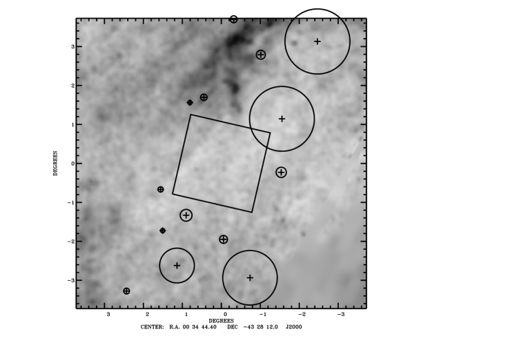
Figure 1: The sky position and orientation of the ISO S1 survey region overlaid on the COBE normalized IRAS maps of Schlegel et al. (1998). The rectangle delimiting the S1 area is $2^{\circ}\times 2^{\circ}$. IRAS sources with 12 $\mu$m flux brighter than 0.6 Jy are also plotted, with radius proportional to flux. The maximum 100 $\mu$m intensity shown (black) is 1.5 MJy/sr.

The ELAIS ISOCAM survey was conducted in raster mode with the LW2 (6.7 $\mu$m) and LW3 (15 $\mu$m) filters. The ISOCAM detector was stepped across the sky in a grid pattern, with about half detector width steps in one direction and the whole detector width steps in the other. In this way, the reliability was improved as each sky position was observed twice in successive pointings and the overheads were reduced because each raster covered a relatively large area (40${}^{\prime}\times 40^{\prime}$). At each raster pointing (i.e. grid position of the raster) the 32$\times$32 ISOCAM detector was read out several times. Table 1 describes the observation parameters for the LW3 filter.

Table 1: S1 LW3 observation parameters

Parameter	LW3 (15 $\mu$m)
Band width	6 $\mu$m
Detector Gain	2
Integration time	2 s
Number of exposures per pointing	10
Additional number of exposures to stabilise	80
Pixel field of view	6′′
Number of pixels	32 $\times$ 32
Number of horizontal and vertical steps	28, 14
Step sizes	90′′, 180′′
total area covered	3.96 deg2

3 Lari Technique: Generalities

As already described in detail by Starck et al (1998), ISOCAM data obtained with the long wavelength detector (LW) are affected by several problems. The two main effects, which become more important the deeper we push for source detection, are produced by cosmic ray impacts (‘glitches’) and transient behaviour (slow response of the detector to flux variations).

Usually, ‘glitches’ can be divided into three categories: common, faders and dippers, according to their behaviour, decay time and influence on the pixel responsivity. Slow decreases of the signal following cosmic ray impacts are called faders, while depletions in the detector gain, followed by a reduction of the pixel sensitivity very slowly recovering afterwards (see figure 2, $top$ panel), are called dippers. These two effects are believed to be associated with proton or $\alpha$ particle impacts on the detector, while cosmic ray electrons produce common ‘glitches’. Common glitches only last one readout and their decay time is relatively fast (lasting only a few readouts), while faders and dippers have much longer lasting impact on the pixel sensitivities. So, the number of frames affected by the latter is much higher than in the case of common glitches, the sensitivity of pixels taking from tens to hundreds of seconds to recover completely. However, common glitches are much more frequent than faders and dippers and, if not correctly removed, they may look like sources on the maps and produce false detections. For this reason, the data cleaning is an extremely delicate process, which requires great care in order to produce highly reliable final maps and source lists.

The LARI method was mainly developed to overcome the main problems affecting ISOCAM LW data and to give better quality maps and as complete and reliable source catalogues as possible. Analogously to the PRETI method (Aussel et al. 1999), our algorithm corrects the cube of ISOCAM data for cosmic rays and transient effects before reconstructing the images and carrying out source detection.

The model on which the LARI method is based (described in detail in Appendix A), rests on the assumption that the incoming flux of charged particles generates transient behaviour producing two different time scale effects: a fast (breve) and a slow (lunga) one. The latter component accounts for the slow response of the detector and is essential in recovering the transient effects of the dippers. Each of the two time scales is associated with an independent reservoir of charge, which decays with this characteristic time-scale towards the contacts (i.e. a multi-component model for semiconductors). These two reservoirs of charge are fed by both incident infrared photons and cosmic rays. The latter are also able to trigger a fast charge release towards the contacts (‘glitches’). When a cosmic ray particle hits the detector, the quickly-varying charge reservoir breve is on average increased, while the slowly decaying charge reservoir is quickly forced to release part of its charge content. Thus, while the breve component is fed by a large fraction of the incident photons (around 40-45 %), the lunga one is fed only by a few percent of them. The remaining fraction is very quickly forced towards the contacts (prompt component). Due to differences between the two time scales of about a factor of 20 when the process reaches stabilisation, the lunga component collects a higher total amount of charge with respect to the breve one.

The value of both time constants depends on the signal level (which is fixed by observations) such that the lower is the signal, the larger is the time constant. Our model simply assumes the time constant to be inversely proportional to the amount of accumulated charge.

To first order, faders are described in this model as discontinuities mainly in the breve charge reservoir, caused by the cosmic ray impact. Similarly, to first order the dippers are discontinuities mainly in the lunga charge reservoir. The maximum depth of the dippers is determined by the fraction of the flux feeding the lunga reservoir. The overwhelmingly large majority of pixels are well-fit by a lunga fraction of $\sim 0.1$, implying that dippers cannot exceed one-tenth of the sky background level. Very occasionally however some dippers exceed this threshold. To account for these, an additional zero-point dark current ‘offset’ can be set, so the maximum depth is not larger than one-tenth of the revised total background. Incidentally, the presence of dippers in the dark current records (that have zero background) shows that this ‘offset’ is a general property of the detector, almost certainly fed by the thermal noise.

4 Application to ISOCAM LW ELAIS data

The application of our model to the ISOCAM LW data obtained in the ELAIS fields required some particular adaptation of the algorithms and the construction of some ‘ad hoc’ procedures necessary to overcome the specific problems generated by the chosen observational strategy.

The main cause of problems in the ELAIS data is the very short integration time. In fact, the time spent by the detector on each readout in these observations is only 2 seconds (see Table 1) and the total time spent on each raster pointing is 10$\times$ the integration time. The short observing time over each raster position (10$\times$2 sec) not only affects the signal-to-noise ratio, but it has two major negative effects on the data:

• since it is shorter than the fast time scale, it makes strong glitches hide real sources;

• only a fraction (60%) of the total incoming flux is recorded during each exposure, thus causing large photometric errors.

In our model, glitches are treated as discontinuities in the charge ($Q$) reservoir, with constant parameters $a$ and $e$ (see Appendix A). However, immediately after the maximum of a glitch, the detector is considered to behave normally under a constant (over the raster pointing) flux $I$. This is not completely correct for very strong glitches, which may cause the signal immediately following the maximum to be higher than predicted and this is mostly true for short integration time observations (i.e. 2 seconds like ELAIS).

Moreover, the relation between the increment of the breve component and the decrement of the lunga one is not constant. In fact, cosmic rays producing a higher increment in the breve reservoir than in the lunga one look like faders, while in the opposite case we have dippers. In the ELAIS data there are dippers without an initial glitch spike: generally we find the glitch feature in a contiguous pixel but, very rarely, it is completely absent.

Another problem arises from the fact that the Point Spread Function (PSF) is spatially under-sampled in all ISOCAM LW3 observations with pixel-field-of-view (PFOV) lens greater than 1.5 arcsec (in our case PFOV = 6 arcsec). Thus, any position determination method applied to individual point sources gives biased results for under-sampled data (the worse sampled the data, the more the resulting position is centered on a pixel). This bias can be corrected to some extent and the source position can be improved up to a fraction of the pixel size by taking into account the a priori raster pattern. In any case, the PSF is not unique for all sources, but it depends strongly on the source location within a pixel. This PSF, corresponding to the position of a source in the raster map and with an average FWHM of $\simeq$10^``, will be referred as “effective PSF” throughout the paper. Moreover, in the ELAIS data each pixel in the final raster map comes from the combination and projection on the sky of different overlapping single images. For this reason, a source in the raster map is produced by the combination of different source images, where the source has different flux distributions, depending on its location within the pixel of the single images. This is a serious problem which affects source detection, source photometry and the completeness of the catalogue. In this work, we have carefully analysed and tried to quantify this combination effect by performing simulations (see section 5).

4.1 ELAIS Data Reduction with the Lari Method

All the codes developed for data reduction with the LARI method are written in the Interactive Data Language (IDL) and the whole data reduction and analysis has been performed with IDL software. The main process of ISOCAM LW data reduction with the LARI method consists of several basic steps. First, the raw data are converted into a raster structure containing all the information about the observation (pointings, instrument configuration, etc.) as well as the single images (one for each pointing, which are combined together to give the final raster image). The images are then converted to ADU/gain/s and the dark current subtracted. These first two steps are performed using the CAM Interactive Analysis (CIA) package. Next, the data are corrected for short time cosmic rays and the affected readouts are masked before copying the “de-glitched” data to a new structure (called “liscio”). This structure contains also the initial guess for the parameters defining the lunga and breve reservoirs of charge and information about the main ‘glitches’ and ‘dippers’ (derived by the deglitching process). The task which performs the first guess for parameters, also evaluates the background and the minimum ‘offset’ to be added to the data in order to have the ‘dipper’ depth in the range allowed by the model (one tenth of the sky background, see section 3). This is done for each pixel. The code not only finds the stabilization background level, that is, the zero level for data fully recovered from transients, but models the ‘glitches’, the sources and the background with all the transients over the whole pixel history. Moreover, our code is able to predict the trend we would have on each raster position if only the stabilization background flux was hitting the detector (starting from the previously accumulated charges, i.e. the ‘local background’). The excess with respect to this ‘local background’ represents the flux excess not recovered from transients. The maps of this excess, after flat fielding, are called ‘unreconstructed’ maps and (in case of a good enough fit) represent the effective flux collected by the detector during the raster exposure. In this paper, fluxes obtained from ‘unreconstructed’ maps will be named fs, while fluxes measured on ‘reconstructed’ maps (i.e. reconstructed from transient effects) will be named fsr. These two fluxes that we can measure for a source are shown in figure 2($bottom$ panel): the dot-dashed line represents the ‘unreconstructed’ data, while the dashed line represents the data ‘reconstructed’ for transients.

With our code, we created a model data-set for the deglitched data, reproducing not only the source signal, but also all the transient effects affecting the data. In figure 2 an example of pixel history is shown, together with the background and data models obtained with our algorithm.

Figure 2: Example of real and model data through the pixel history. The solid line represents the data and the dot-dashed line the best-fit model, while the dashed line is the data corrected for transients and deglitched. The dotted horizontal line is the assumed background level. In the $top$ panel the characteristic ISOCAM LW transient behaviours due to cosmic rays are shown. The raw data are clearly affected by many ‘glitches’, as well as by strong ‘dippers’ and ‘faders’, and by upward transients. The $bottom$ panel is a zoom in the history of a pixel, which shows how our model works in fitting the data and reconstructing the stabilized signal when the pixel sees a source.

In outline, the fitting algorithm starts with the brightest glitches in the raster, assumes discontinuities at these positions, and tries to find a fit to the time-lines that satisfies the solid-state physics of the detector. If no acceptable fit is found, the next fainter glitch is considered as a potential discontinuity, and so on. Because of the reduced number of useful readouts in the ELAIS raster data, in the fit we use fixed default values for all the pixels (the physical parameters scaled only for the background level), leaving as free parameters only the charge values at the beginning of the observations and at the top of glitches.

By successive iterations, the parameters and the background for each pixel are adjusted to fit the data better, until the rms of the difference between model and real data is smaller than a given amount (e.g. 0.2 ADU/gain/s ). Note also that the effects generated by the presence of glitches in the nearby pixels are considered by the fitting algorithm. The code recognizes sources above a given flux level, which decreases as the reduction improves the fit. In the pixels around relatively strong sources ($>$ 1.3 ADU/gain/s) we force the fit to find sources, leaving the fit level free. Once a satisfying fit is obtained for all the pixels over the whole pixel history, the flat field is computed from the stabilization level of the background. In the raster structure we set the flat fielded smoothed differences of: a) data readouts minus local fitted background (‘unreconstructed data’); b) fully recovered intensities minus stabilization level (‘reconstructed data’). Glitches and bad data are masked and this mask is stored in the raster structure to be used later in the map creation.

Then the reduced images per raster pointing are computed and corrected for flat-field distortions. Finally, the images are combined together to create the final raster maps (one for each raster position), where we then look for source detection.

A final reduction stage is performed after source extraction, simulating the data we would have from these detections and correcting the pixel fit, forcing the algorithm to recognize the source whenever this had not happened correctly (i.e. the source had been recognized only in one of the two overlapping single pointing images and not in the other).

We will now enter into more detail on the map creation and source detection processes.

4.2 Map creation

Once the images, corresponding to each raster position, have been created by averaging together all the time-scans relative to that pointing, they are converted from ADU/gain/s to mJy/pixel using the ISOCAM User’s Manual calibration factor (e.g. dividing by 1.96) and flat fielded. Also the number of un-masked times-scans (raster.npix) are scaled with flat-field coefficients, on the simple assumption of a constant noise in the data prior to flat-fielding.

After that, they are projected onto a sky map (raster image) using a simple TAN projection. The algorithm used is part of the CIA package (projette.pro). It computes the values of pixels on the sky map by averaging the pixel values in the single images, with a weight equal to the number of useful time-scans, to give the pointing image (raster.npix). For each raster map, two corresponding maps are also constructed, with the same size and sky orientation. One is the map containing, for each pixel, the number of frames coadded together (excluding the masked pixels) to obtain that pixel value in the raster (“NPIX” map). The other is the “RMS” map, where the rms of each pixel has been computed by scaling the measured mean rms of the central part of the map according to the inverse square root of “NPIX”.

In projecting each raster pointing onto the sky, the algorithm takes into account the field distortions of ISOCAM, as measured by Aussel et al. (1999). These distortions are a chromatic effect which cause the pixel size to be non-uniform on the sky (border pixels are larger in area than central pixels). This effect must be considered also when computing the flat-field. For a more detailed description of the ISOCAM field distortions see Okumura (2000).

In figure 3 the grey-scale image of the central raster map (S1$\_$5) is shown. Note that this image, $S1\_5$, is the combination of three single observations, this field having been observed with a redundancy of 3 compared to the other rasters.

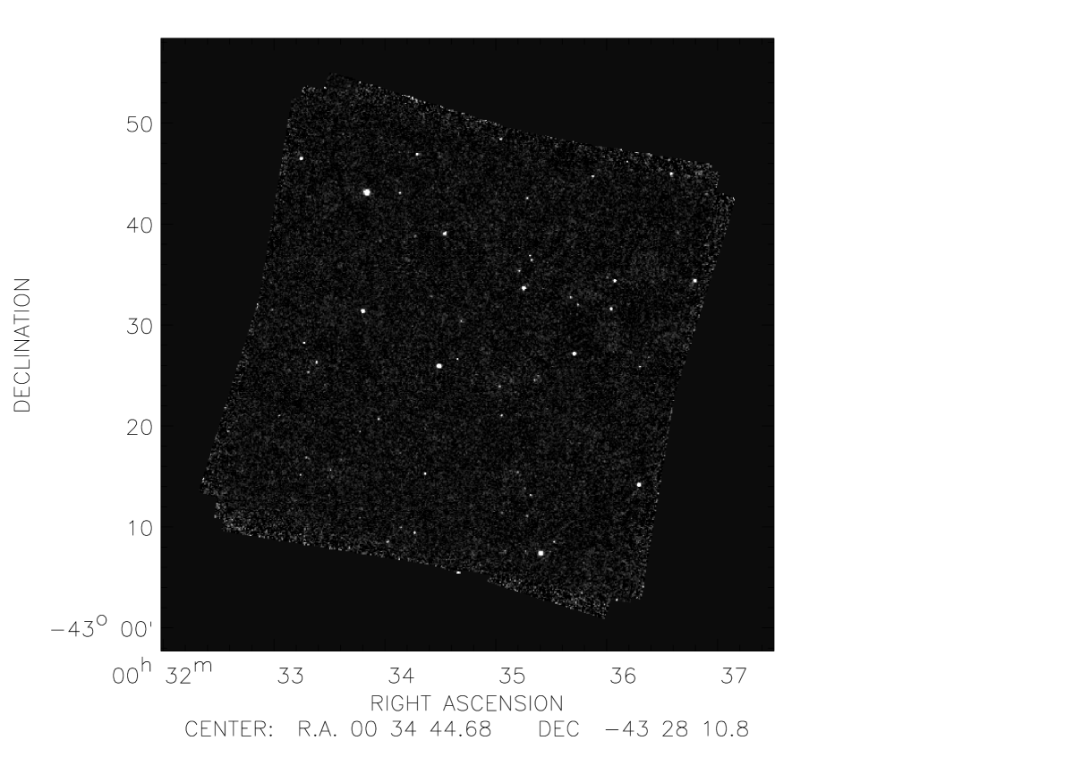
Figure 3: Grey-scale image of the central raster $S1\_5$. This map derives from the combination of three single observations and the higher noise level at the borders, where the overlap between the three pointings is not perfect, is clearly visible.

The projection algorithm strongly affects the appearance of point sources on the map, having the general effect of smoothing the PSF over several pixels. As we will show in section 5.2, the peak flux values of sources with the same total flux can differ significantly, by a factor of up to 2, depending on the source position within the raster pixel.

4.3 Source detection

Before performing the proper source detection (on the final maps) to produce our definitive source catalogue, we have identified candidate sources inside the pixel histories. This was also very useful to check the confidence level of our fit to the data. Since during data reduction we have created a model for the background, we identified sources in the history of pixels from their flux excess above the background over the single time-scans. We inspected by eye every excess greater than 0.7 ADU/gain/s, correcting the few cases corresponding not to real sources, but to algorithm failures (by re-setting the parameters and starting again with model fitting until convergence is achieved). We have found that our method is very conservative, in the sense that cases where a spurious source is created by the algorithm constitute a very small fraction of the total number of correct detections, while the fraction of good sources missed by the fitting algorithm is rather significant (since sources are normally seen on several pixels, a lost detection on the pixel history does not necessarily mean the source is lost on the map).

Only faint sources remaining undetected on the map (because of these failures) contribute to real incompleteness, while for most of the brighter sources the failures result in a decrease of their total flux. In the final stage of our reduction (see below), we re-project the sources detected on the raster map into the pixel time-line, allowing a better fit of the data for all the sources that will appear above the interactive check threshold. This job significantly reduces the flux defect for the detected sources (but is of course unable to recover sources that fell below the detection threshold, i.e. to correct for incompleteness).

Concrete determination of the fraction of detected sources versus real sources, which leads to the estimate of completeness and reliability of our source catalogue, have been performed using simulations. This will be discussed in section 5.

After this preliminary check, we have searched for detections in the single calibrated images by selecting and visually inspecting all pixels with flux $>0.4$ mJy / pixel. In this case too, we have performed again the reduction for those pixels where the algorithm had failed to fit the data, thus producing a false detection.

These two checks on candidate sources, which required corrections and further cleaning for some pixels, provided very reliable (not complete!) source lists and images. After that, we could be confident that almost no spurious sources were present in our data-set. Therefore, we could proceed to the proper source detection. We must now point out that all the checks performed on the single pointing images and pixel histories do not guarantee that all these (and only these) sources will then be detected on the final raster map. In fact, as already discussed, the raster pixels are produced by combining together different single pointing images, where the same source could be located in different positions inside the pixels, thus being for example above the 0.4 mJy/pixel check threshold in one image and below this threshold in the other. For this reason, the list of sources obtained in the single pointing images for our preliminary checks are not always coincident with the final list derived on the raster map, where each source is determined by different effects. Moreover, in the raster map creation there are also distortion effects. Thus, the completeness and reliability of our final source lists can be tested only through simulations.

The source detection is done on the final raster maps, but is done using the signal-to-noise ratio. First, we have selected all pixels above a low flux threshold (0.1 mJy / pixel) using the IDL Astronomy Users Library (accessible via the World Wide Web home page http://idlastro.gsfc.nasa.gov/homepage.html) task called find. This algorithm finds positive brightness perturbations (i.e. stars) in an image, returning centroids and shape parameters (roundness and sharpness). Then, we have extracted from the selected list only those objects having a signal-to-noise ratio $\geq$ 5.

As discussed earlier, the LARI method is able to ‘reconstruct’ the source flux from transient effects. However, as we will clearly show with simulations (see section 5.2), the algorithm does not ‘reconstruct’ faint fluxes, corresponding to sources that it is not able to recognize. Therefore, faint sources have ‘reconstructed’ fluxes similar to their ‘unreconstructed’ ones, while for bright and correctly ‘reconstructed’ sources the ‘unreconstructed’ flux is, on average, about 1.7 times smaller than the corresponding ‘reconstructed’ flux. For this reason, to have a homogeneous flux determination for all our sources (both bright and faint), we have chosen to run the detection algorithm on the ‘unreconstructed’ maps. The correction for transients effects has then been performed individually in a second step, by using for each source its “effective PSF” when deriving its total flux (“auto-simulation” procedure, see section 5.1).

In order to achieve better position determination, we have run the detection algorithm on higher resolution maps, obtained by re-binning the original raster maps with a pixel size of 2 arcsec. The positions and fluxes given in output by find are determined by a convolution with a Gaussian PSF of given full width at half maximum (FWHM). We have chosen a FWHM = 9.8 arcsec, which is slightly smaller than the average FWHM of the ELAIS LW3 “effective PSF”.
The fluxes given by find are peak fluxes (mJy / pixel), which, coming from a Gaussian convolution, do not always correspond to the real source peaks. Therefore, for source peak flux (fs) we have given the maximum pixel value found within a box of 4 $\times$ 4 arcsec around the maximum given by find. To obtain the total fluxes (in mJy) we have used (and compared) two different methods: direct aperture photometry on the maps and “auto-simulations”, as discussed in detail in section 2.

5 Simulations

Because the raster maps on which we have performed the source detection are derived from the combination of several single pointing images, the only way to evaluate the effects produced on sources in the combined maps is through simulations.

With simulations, we can study the completeness and reliability of our detections at different flux levels and estimate the source positional accuracy and the internal calibration of the source photometry.

We added randomly distributed point sources to each of the three overlapping central raster maps (S1$\_$5, S1$\_$5$\_$B and S1$\_$5$\_$C) at five different total fluxes (200 at 0.7, 150 at 1, 200 at 1.4, 150 at 2 and 150 at 3 mJy). It must be pointed out that our simulations have not been performed over the entire flux range covered by our survey, but only at the faint end. The reason is that we choose to sample with a high statistical significance the flux range more affected by incompleteness effects due either to mapping undersampling or data reduction method failures.

In a similar way we get simulations on the combined mosaiced map for which we have 50 sources at the same five flux levels.

To perform the simulations, we have created a high resolution map ($1^{``}$) with simulated source, taking the ISOCAM PSF into account. The PSF has been successfully modeled by Okumura (1998) for stars. The PSF varies with the wavelegth, and since the ISOCAM filters are large, the shape of the PSF depends on the assumed spectrum of the point source. For our purpose, we have recomputed a model, following the prescriptions of Okumura (1998) but using a spectrum of the form $f_{\nu}=constant$, that is a closer match to the expected galaxy spectrum than the Rayleigh-Jeans form used for stellar spectra. The resulting PSF is larger than the one computed on stars.

Inverting the flat field and converting in ADU/gain/s we obtained the flux excess corresponding to the simulated sources. The value of this flux excess was then added to the real pixel histories (containing glitches and noise) by using Lari model, to obtain the simulated data cube. This simulated flux, included in the “liscio structure” (see section 4.1), have been reduced exactly in the same way as we did for all the original data structures, doing the same checks and repairs. In the produced maps we extracted the simulated sources with the same procedures used for the real rasters, measuring the resulting positions and peak fluxes. The peak fluxes measured after the data reduction will be referred as fs and fsr (as well as for real sources) respectively for ‘unreconstructed’ and ‘reconstructed’ maps. The corresponding theoretical peak fluxes associated to the excess flux maps, not reduced and containing neither glitches or noise, will be named f0 and f0r. These two sets of parameters then allow to evaluate separately the effects produced by the ELAIS observational strategy and the ISOCAM instrument only (f0 and f0r; see section 5.1) from the effects produced by the LARI reduction method applied to ELAIS data (fs and fsr; see section 5.2).

5.1 Theoretical transient behaviour of the detector

By simulations of the theoretical transient behaviour of the detector, we mean simulations of the effects due to the finite spatial resolution (6 ^′′) and to the finite integration time (10$\times$2 sec) of our observations. We need to consider the spatial resolution of our observations, since the PSF is comparable in size to a pixel, causing the observed point source to depend strongly on its position on scales smaller than the pixel size.

Regarding the finite integration time, we need to simulate the fact that the CAM detector does not reach immediately the level corresponding to a given input flux, but needs a certain time to stabilize (see section 3). This stabilization effect, which means that only a fraction of the incident flux is detected, is not constant, but depends on the length of the time spent by the detector on target (not always the same) and on the amount of masking in a pixel (due to ‘glitches’ and uncertainties on the time spent on positions).

With the positions measured on simulated maps we can simulate how sources would appear in the ELAIS rasters if no noise and ‘glitches’ were present. To do this, we created two maps for each raster. The first is obtained by projecting back the simulated sources, injected on measured positions, onto the single pointing images and then computing the resulting raster map. The peak fluxes measured on it are the ‘reconstructed’ peak fluxes: $f0r$. For the second map we went back to the pixel history, predicting the behaviour due to the finite integration time transient (only theoretical, without any noise) and then producing a raster map. The peak fluxes measured on it are the ‘unreconstructed’ peak fluxes: $f0$.

Figure 4: Distribution of normalized peak flux for mapping effects only, $f0r/flux$, and for mapping $+$ source transient, $f0/flux$, for all the 850 simulated sources .

Figure 4 shows the distribution of the peak fluxes (‘unreconstructed’ peak flux: $f0$; ‘reconstructed’ peak flux: $f0r$) normalized to 1 mJy (divided by the corresponding input flux, i.e. the effective PSFs), for simulated sources. The effect of mapping is the main responsible for the large spread of values in the figure, because the distribution of the $f0r/f0$ ratios has a rms of only 0.09 (0.05 for the repeated field S1$\_5$) around a mean value of 1.66. The position uncertainty is only a minor contributor to the observed spread, since it causes only $\sim$14% of the $f0$ and $f0r$ distribution dispersion.

The ratios of sources detected over the total number of injected sources, due to PSF under-sampling and finite integration time are reported in the second column of Table 2 for each input flux.

The simulation of the mapping and mapping $+$ transient effects provides the estimate of the individual PSF for each source and gives a technique to be used to derive total fluxes for all the sources: for each source we will have two individual PSFs, one from $f0r$ and one from $f0$.

As we will show in section 2, there is a tight correlation between the peak flux of a source and its theoretical peak flux due to mapping and transients only (“effective PSF”). These “effective PSFs” can be used for aperture flux determination (using small radii) and we will show that the total fluxes derived from the observed peak fluxes correspond very well to the aperture photometry ones.

5.2 Real transient behaviour of the detector

Since the data reduction method can cause incompleteness in the final source list, we must take into account the effects produced by the fit when deriving the corrections to be applied to our catalogue. In fact, our data reduction method is based on a fitting algorithm and, depending on how well this is able to model the background, the ‘glitches’ and the sources, our catalogue will be more or less complete. For this reason, with simulations we have also tested the effects of Lari model on the final data products.

As stated above, to test the data reduction method, we have followed the same procedure for the simulated data that we used for real data. These simulated data cubes contain both real sources and simulated ones. They have also the same rms noise, all the ‘glitches’, ‘faders’, ‘dippers’ and background transients as the original data. The confusion will be slightly increased, but this effect is not critical for ELAIS data.

By comparing the output fluxes (per pixel) obtained for the simulated sources affected only by the mapping effects ($f0$) with the output fluxes of the reduced simulated sources ($fs$), we find a correlation (although not a 1 to 1 correlation, since the reduced fluxes are always slightly lower than the unreduced ones, see figure 5(top)). A similar correlation is observed for the corresponding ‘reconstructed’ peak fluxes ($f0r$ and $fsr$, reconstructed from the transients), although for faint sources our algorithm is not able to reconstruct correctly the fluxes (see figure 5($bottom$)).

Figure 5: top - Output flux after reduction versus output flux due only to sampling effects for simulated sources. The fluxes are ‘unreconstructed’ for transients. The open circles represent the sources detected above 5 $\sigma$, while the dots are the sources below the 5 $\sigma$ threshold. bottom - ‘Reconstructed’-to-‘unreconstructed’ flux ratio ($fsr/fs$) normalized to the same ratio obtained for mapping effects only ($f0r/f0$) as function of the detected ‘unreconstructed’ peak flux. The ratio distribution broadens towards lower values at faint fluxes, due to the characteristic of LARI method of not reconstructing faint sources.

The dispersion of values in figure 5(top) is caused by two kind of errors:

• an error proportional to the flux caused by the reduction method limits or by the mapping and finite integration time effects. In either cases, this error affects the peak fluxes.

• an additive error caused by the presence of noise and confusion. This error is more effective at low fluxes than at high ones.

At low fluxes, the combination of these errors may cause the total loss of a source (i.e. incompleteness).

Figure 6: Distribution of the ratio between the reduced peak flux and the unreduced peak flux (derived from mapping effects only), $fs/f0$, for all the 424 simulated sources detected above $5\sigma$ (dot-dashed line marked by diagonal crosses) and for the 147 detections injected at 3 mJy (solid line marked by diamonds).

Figure 7: Predicted distributions of the ratio between the reduced peak flux and the unreduced peak flux (from mapping effects only), $fs/f0$, computed in presence of a noise of 26 $\mu$Jy. These distributions are shown for three different average values of $f0$ corresponding to different input fluxes (i.e. $<f0>=605~{}\mu$Jy for an input flux of 3 mJy).

Figure 6 shows the distribution of the ratio between $fs$ and $f0$, for the 424 simulated sources detected above $5\sigma$, compared to the same ratio for the 147 detections at 3 mJy only. As already noted in figure 5($top$), the ratio is not centered on the value of 1, thus causing a general underestimation of the total fluxes (derived from $fs$). There are two reasons for this effect: one is the fact that $f0$ is computed on the measured positions of $fs$ (about 11% higher than on real positions); the other is the under-evaluation of the wings of faint sources by the LARI method. The former effect is caused by the fact that projection effects cause $f0$ to be enhanced at favorable positions (i.e. center of a pixel on the single images), affecting also the centroid position even in the absence of noise. This overestimates the peaks of simulated sources which do not fall on the center of a pixel, thus leading to a bias in the ratio between the real $f0$ peak flux and the measured $f0$ simulated peak flux. The values of $f0$ computed at the positions measured for $fs$ are on average $\sim$11% higher than the ones computed at real positions.
The total distribution is larger and with a longer tail than the 3 mJy one. This is caused by the noise contribution to the errors, which is more significant at low than at high fluxes, as shown in figure 7. In this plot, the predicted distributions of the ratio $fs/f0$ in presence of a noise of 26 $\mu$Jy are shown for three different values of $f0$, corresponding to different mean values of $f0$ for different input fluxes (i.e. $<f0>=605~{}\mu$Jy for 3 mJy input flux). As we can notice, the presence of noise broadens the flux distributions and this effect becomes stronger towards fainter fluxes. The predicted and unbiased distribution of $fs/f0$ for the brighter sources (3 mJy) peaks at 0.78 $\pm$ 0.03, value subsequently assumed to correct our measured fluxes (see section 2).

If we assume that the 3 mJy distribution reflects all the multiplicative error components due to the data reduction and we correct for the noise effect, we can predict the distribution of the detection rate for all the total and peak fluxes considered and derived in the simulation. Figure 8 shows the ratio of found-to-predicted detections as a function of $f0$, with the predictions obtained by considering two sources of error: (1) the multiplicative errors only (due to the reduction method and mapping, see section 2; solid line); (2) the multiplicative errors plus the additive noise contribution, assuming a typical noise level on maps of 26 $\mu$Jy (dashed line). It is visible a decrease of detection rate/predicted rate below $\sim$300 $\mu$Jy/pixel, which corresponds roughly to 1.5 mJy in total input flux. This deficiency is the nominal incompleteness of our data reduction method.

Figure 8: Found-to-predicted detections ratio as a function of $f0$. The predictions have been obtained by considering the multiplicative errors only (due to the reduction method and mapping, see section 2; solid line); the multiplicative errors plus the additive noise contribution, assuming a typical noise level on maps of 26 $\mu$Jy (dashed line).

The detection rates at different fluxes derived with our simulations are reported in Table 2, where the predictions if only mapping smearing would be present, the predictions considering the data reduction but without taking into account the incompleteness of our method (see figure 8), the predictions considering also the incompleteness curve and the found values are given as detection fractions (i.e. detected sources / input sources) for the five different input fluxes. In figure 9 the detection rate curves relative to the values given in Table 2 are shown as function of the input flux.

As shown both in Table 2 and in figure 9, almost all the injected 3 mJy sources are detected at $\geq$ 5$\sigma$. Thus, the detection rate is 98.7% above 3 mJy, and it remains above 85.9% at 2 mJy. However, the detection rate drops quickly at fainter fluxes, in fact it reaches 52.3% at 1.4 mJy and 24.8% and 4.4% at 1 and 0.7 mJy respectively. Both sampling and reduction method are responsible for the large source undetectability at faint fluxes, although the contribution due to LARI method seems to become more important around 1.4 - 1 mJy, then it keeps almost constant, while the PSF sampling effect significantly decreases the detection rate for fluxes fainter than 1 mJy.

Table 2: Detection rates

input flux	predicted(mapping)		predicted(map+reduction)		predicted(map+red+incompl)		detected
(mJy)	over injected	(%)	over injected	(%)	over injected	(%)	over injected	(%)
0.7	42.5/198	21.5	21.8/198	11.0	5.5/198	2.8	8/198	4.0
1.0	114.4/149	76.8	71.5/149	48.0	33.0/149	22.1	37/149	24.8
1.4	195.2/199	98.1	164.4/199	82.6	109.0/199	54.8	104/199	52.3
2.0	148.3/149	99.5	144.2/149	96.8	126.0/149	84.6	128/149	85.9
3.0	148.5/149	99.6	148.2/149	99.4	145.4/149	97.6	147/149	98.7

Figure 9: Percentage of detected sources in simulations of ELAIS S1 as a function of the source input flux. As detection threshold we have considered 5$\sigma$. The dash-dotted curve represents the effect of PSF sampling on the detection rate; the dashed curve represents the effect of the LARI method; the solid curve is the total effect on reduced LW3 ELAIS data.

It must be pointed out that these incompleteness factors cannot be directly translated to the real catalogue, which has not a monochromatic flux distribution as the simulations. These factors can however be used to obtain the completeness of the catalogue and the source counts corrections, assuming a model for the $logN-logS$ (see Gruppioni, Lari, Pozzi et al. 2001). When applying simulations to real sky maps we must also remember that there are other sources of error not included in the simulations, as flat field corrections and distortion tables. The latter causes a higher smearing of the images and a larger uncertainty on centroid positions.

6 Flux determination

The simulation procedure described in section 5.1 has been used also to estimate the effective PSF on a source, real or simulated, and its total flux, given its position and peak flux. This procedure, performed on sources to determine their total flux from their peak flux and position is called “auto-simulation”.

The linear relation existing between $fs$ and $f0$ (see figure 5($top$)) allows the definition of a flux estimate for both simulated and real sources:

$$f_{total}=fs\times(flux/f0).$$ (1)

While for simulations $flux$ is the injected total flux, for real sources we need to adopt a rough estimate for $flux$ to derive $f_{total}$. $Flux$ is the total injected flux used to compute $f0$ (for simulations is 0.7, 1, 1.4, 2 and 3 mJy). Since transient corrections depend (slowly) on $flux$, for real sources we started with a rough estimate for $flux$ and then we iterated equation 1 to obtain a good estimate of $f_{total}$ also for strong sources.
The starting rough estimate of $flux$ is obtained by:

$$flux=fs/<fs/flux>_{sim}$$ (2)

where $<fs/flux>_{sim}$ = 0.132 was the average value taken from simulations.
Given this input total flux, we can derive $f0$ for real sources exactly as we did for simulated sources (see section 5.1). Then, by using formula 1, corrected for the systematic bias of the $fs/f0$ distribution (i.e. divided by 0.78; see section 5.2), we obtain the value of the total flux, $f_{total}$, for our sources. Given the relation 1, figure 5 could also be seen as the representation of the $f_{total}/flux$ (i.e. measured flux / true flux) distribution.

In figure 10 the total fluxes obtained with this procedure are plotted as function of the reduced peak fluxes obtained for all the simulated sources. As in figure 5, the open circles represent the sources detected above 5 $\sigma$, while the dots are the sources below the 5 $\sigma$ threshold.

Figure 10: Total fluxes obtained with the auto-simulations versus reduced peak fluxes for simulated sources. The open circles represent the sources detected above 5 $\sigma$, while the dots are the sources below the 5 $\sigma$ threshold.

The total fluxes obtained with the auto-simulations for the simulated sources are then compared with the total fluxes obtained with aperture photometry of the same simulated sources.

Concerning the aperture photometry fluxes, we found that the better determination was achieved with an aperture radius of 8<sup>``</sup>, after correcting for the missing flux outside the aperture (40% in the PSF wings at distance $>8^{``}$). We have found a good agreement between the two flux determinations (see figure 11 for a comparison between the two results). As total flux estimates for our real data sources, we have then decided to adopt the fluxes obtained from the auto-simulations.

In addition to the systematic bias affecting the $f0$ measured values, there is also a flux-dependent bias at low signal to noise levels, which derives from the fact that only sources with a high $fs/f0$ value and with positive noise fluctuations can be detected. However, only constant bias corrections are applied to our catalogue data.

Figure 11: Aperture photometry flux normalised to its relative effective PSF versus total flux obtained with auto-simulations for simulated sources.

6.1 Flux errors

As already mentioned in section 5.2, there are two main sources of uncertainty on our source fluxes: a multiplicative error due to mapping and data reduction method and an additive error due to the presence of noise in the map (neglecting the uncertainties due to flat-fielding corrections and field distortions, the latter always depressing the peak fluxes). As mentioned in section 5.1, the spread in the $f0$ distribution caused by position errors is about 14%. This spread is not only an important cause of the total flux bias, but it contributes significantly to the width of the $fs/f0$ distribution ($\simeq$0.18) at high fluxes. The extra contribution from data reduction is about 11%. Since simulations show that this spread is rather insensitive of fluxes, we assumed that the multiplicative error is constant.

Because our total fluxes are obtained from the ratio between peak fluxes and auto-simulated peak fluxes, the combination of the two errors leads to a flux-dependent distribution like the one shown in figure 8.

Being the width of the $fs/f0$ distribution equal to 0.18 at high signal to noise levels, the distribution convolved with noise will have a width:

$$w^{2}=(0.18)^{2}+(rms/f0)^{2}$$ (3)

We used this relation to obtain the relative flux errors for sources.

7 Test of the photometry

The photometric accuracy of our reduction of the S_1 area can be tested using the stars of the field. Aussel & Alexander (in prep.; see also Alexander & Aussel, 2000) have performed a detailed study of the mid-infrared emission of stars, from large sample of sources drawn from the IRAS Faint Source Calalog with excellent counterparts in the Tycho-2 catalog (Hog et al., 2000). They show that the B-V color of stars is extremely well correlated with the B-[12] color, where [12] is a magnitude scale constructed from the IRAS flux, following the prescriptions of Omont et al. (1999). This relation allows to predict accurately the 12 $\mu$m IRAS flux of a star, provided that its B-V is known, and is lower than 1.3. Stellar atmosphere models (Lejeune et al., 1998) show that for the spectral types hotter than K3 that the color criteria select, the ratio of the 15 $\mu$m flux to the 12 $\mu$m flux of stars is constant. We have therefore used the relation calibrated on IRAS data by Aussel & Alexander to predict the fluxes of stars in the field, and we compare them to the product of our analysis.

Figure 12: LW3 15 $\mu$m fluxes measured with our analysis for the 63 stars from the Tycho-2 catalogue in the S1 area versus 15 $\mu$m fluxes predicted using the relation calibrated on IRAS data by Aussel & Alexander. Filled circles are the 48 stars with $B-V<1.3$, while crosses are the 15 stars with $B-V>1.3$. The dashed line shows the one-to-one relation.

Figure 13: Measured to predicted flux distribution for a sample of 3950 stars from the study of Aussel & Alexander (IRAS 12 $\mu$m fluxes, dotted line), predicted distribution on S_1 (dashed line) and the distribution of the 48 stars from the Tycho-2 catalogue detected in our analysis of S1 (LW3 15 $\mu$m fluxes).

The area surveyed in S_1 contains 170 stars in the Tycho-2 catalogue, 145 of which with $B-V<1.3$. In our analysis we detect 63 of them, 48 with $B-V<1.3$. We plot on figures 12 and 13 respectively the measured fluxes versus the predicted fluxes and the histogram of the ratio of the measured flux to the predicted flux. In figure 12 the dashed line shows the one-to-one relation, followed by our data over more than two order of magnitude in flux. In figure 13, the dotted line shows the ratio of measured over predicted IRAS 12 $\mu$m fluxes, for a sample of 3950 stars from the study of Aussel & Alexander. The distribution is a skewed log-normal, dominated by the error of the IRAS FSC photometric error of the order of 10% on average. It is skewed toward observed fluxes higher than predicted fluxes, because some stars present an excess of IR emission due to the presence of a disk or shells. Dashed line is the result of the covolution of the former distribution with the $fs/f0$ strong sources distribution to simulate the spread of values we would expect in our analysis, neglecting noise. The mean value of this distribution is 1.047 while the 48 stars in S_1 with $B-V<1.3$ have a mean value of .955 leading to a relative flux scale of $1.096\pm.044$.

The solid line is the ratio of the measured LW3 flux and predicted fluxes for the 48 stars detected in S_1.

The shape of the distribution is the same as the dashed one, apart the small scale factor, with the same skewness and we are confident our fluxes are correct, over a large range of fluxes since these stars go from 0.85 mJy to 135 mJy in LW3.

8 Positional accuracy

The positional errors in RA and DEC for our sources can be considered as the combination of three different sources of uncertainty: the finite spatial sampling ($\sigma_{s}$), the reduction method ($\sigma_{r}$), and the uncertainties in the pointing accuracy ($\sigma_{p}$). The latter is due to errors in the ISOCAM lens position (the wheel jitter) and results in an offset of about 1.2 pixels from the optical axis, that translates to $\sim$7 arcsec with a pixel size of 6^′′. Moreover, ISO absolute pointing accuracy is about 3 arcsec.

The effect of the finite spatial sampling ($\sigma_{s}$) has been evaluated from the “theoretical” simulation (see 5.1), considering the distribution of the differences between the positions of the injected sources (RA,DEC) and the positions of the (same) sources detected in the projected map (RA0, DEC0).
The sum of this effect plus that produced by the method of reduction ($\sigma_{s+r}$) has been evaluated from the “real” simulation (see 5.2), considering the distribution of the differences between the positions of the injected sources (RA,DEC) and the positions of the sources detected in the projected map after the reduction (RAS, DECS). The widths of these distributions are 0.63 (RA) and 0.91 arcsec (DEC) for sampling only and 1.17 (RA) and 1.27 arcsec (DEC) for sampling and reduction effects. In figures 14 we plot the distributions of the differences in RA and DEC between the injected and detected positions.

By using our simulations at different input fluxes, we have also checked the dependence of the positional errors on source signal-to-noise ratio, as shown in figure 15. While the positional accuracy due to sampling only is almost constant with signal-to-noise ($\sigma_{s}\approx$0.9^′′ for DEC and $\sigma_{s}\approx$0.65^′′ for RA), as expected being a pure geometrical factor, the positional accuracy after the reduction is strongly dependent on signal-to-noise, increasing by about 50% from $S/N\geq 10$ to $S/N\approx 5-7$ (i.e. $\sigma\approx$1.0^′′ for RA at $S/N\geq 10$; $\sigma\approx$1.5^′′ at $5\leq S/N\leq 7$). These dependences can be approximated by exponential laws of the form :

$$\sigma_{s+r}(RA)=1.0+17.17\times e^{-(0.57\times S/N)}$$ (4)

$$\sigma_{s+r}(DEC)=1.06+1.21\times e^{-(0.16\times S/N)}$$ (5)

These laws, plotted in figure 15 as solid lines and found with a non-linear least squares fit, have been used to estimate the positional errors due to the mapping and reduction method as a function, for each source, of its signal-to-noise.

Figure 14: Distribution of the difference in RA (top) and DEC (bottom) between the injected and the found positions for the simulated sources. Dashed line: sampling effect; solid line: sampling plus reduction effect.

Figure 15: Positional errors versus signal-to-noise ratio (top: RA; bottom: DEC). Asterisks represent the errors due to mapping effects only, while diamonds are the errors due to mapping and data reduction effects. The dot-dashed lines represent exponential fits to the error dependency on source signal-to-noise ratio.

The errors introduced by uncertainties in the ISOCAM pointing can be estimated by performing optical identifications for the sources found in each raster and computing an offset with respect to the optical astrometric reference system. As optical reference list we have used the PMM USNO-A2.0 Catalogue (Monet 1998).

With between 28 and 36 ISOCAM/USNO coincidences per raster found, we derived the median offsets for each of the 11 frames using the following procedure. First, we have cross-correlated the ISOCAM and USNO lists using a maximum distance of 60 arcsec to obtain the best value for the maximum distance for reliable identification. This distance resulted to be 12 arcsec for all the rasters. Then, for each raster we have obtained the median offset values in RA and DEC ($med_{ra1}$ and $med_{dec1}$) using all the ISO-USNO sources with a maximum distance of 12 arcsec. We applied the offset values to the ISO positions and we have cross-correlated again the ISO and the USNO catalogues.

Table 3: ISO-USNO astrometric corrections

Raster	Nominal Position	RA (′′)	DEC (′′)
	(J2000)	offset    error	offset    error
S1$\_$1	00 30 25.4 $-$42 57 00.3	$-$2.06 $\pm$ 0.40	$-$4.46 $\pm$ 0.38
S1$\_$2	00 31 08.2 $-$43 36 14.1	$-$3.24 $\pm$ 0.22	+6.86 $\pm$ 0.29
S1$\_$3	00 31 51.9 $-$44 15 27.0	+1.57 $\pm$ 0.29	$-$7.75 $\pm$ 0.33
S1$\_$4	00 33 59.4 $-$42 49 03.1	+0.23 $\pm$ 0.22	$-$4.01 $\pm$ 0.27
S1$\_$5A	00 34 44.4 $-$43 28 12.0	$-$3.50 $\pm$ 0.23	+9.63 $\pm$ 0.27
S1$\_$5B	00 34 44.4 $-$43 28 12.0	$-$0.52 $\pm$ 0.21	$-$8.10 $\pm$ 0.26
S1$\_$5C	00 34 44.4 $-$43 28 12.0	$-$3.04 $\pm$ 0.24	+5.34 $\pm$ 0.29
S1$\_$6	00 35 30.4 $-$44 07 19.8	+0.60 $\pm$ 0.43	$-$7.14 $\pm$ 0.24
S1$\_$7	00 37 32.5 $-$42 40 41.2	+1.26 $\pm$ 0.22	$-$5.62 $\pm$ 0.38
S1$\_$8	00 38 19.6 $-$43 19 44.5	+0.72 $\pm$ 0.22	$-$5.31 $\pm$ 0.24
S1$\_$9	00 39 07.8 $-$43 58 46.6	$-$2.34 $\pm$ 0.19	+4.61 $\pm$ 0.23

We have selected again all the sources within a maximum distance of 12 arcsec and we have used these sources to calculate new median offset values ($med_{ra2}$ and $med_{dec2}$). The total offsets for each raster have then been obtained as $RA\_offset=med_{ra1}+med_{ra2}$, $DEC\_offset=med_{dec1}+med_{dec2}$. The values of the offsets and their relative errors (computed as the standard errors on median: $\sigma_{med}=1.2533\frac{\sigma}{\sqrt{N}}$ (Akin & Colton 1970), where $\sigma$ and $N$ are respectively the standard deviation and the number of sources considered in each raster) have been reported in Table 3. Each source position has then been corrected for the offset found for the corresponding raster. The error ($\sigma_{p}$) introduced on source positions by the presence of the systematic offset is given by the error on the offset determination (see column 4 and 6 in Table 3). This error has been added to the positional uncertainty due to mapping and reduction method ($\sigma_{s+r}$) to obtain the total position error for each source:

$$\sigma^{2}_{RA}=\sigma^{2}_{s+r}(RA)+\sigma^{2}_{p}(RA)$$ (6)

$$\sigma^{2}_{DEC}=\sigma^{2}_{s+r}(DEC)+\sigma^{2}_{p}(DEC)$$ (7)

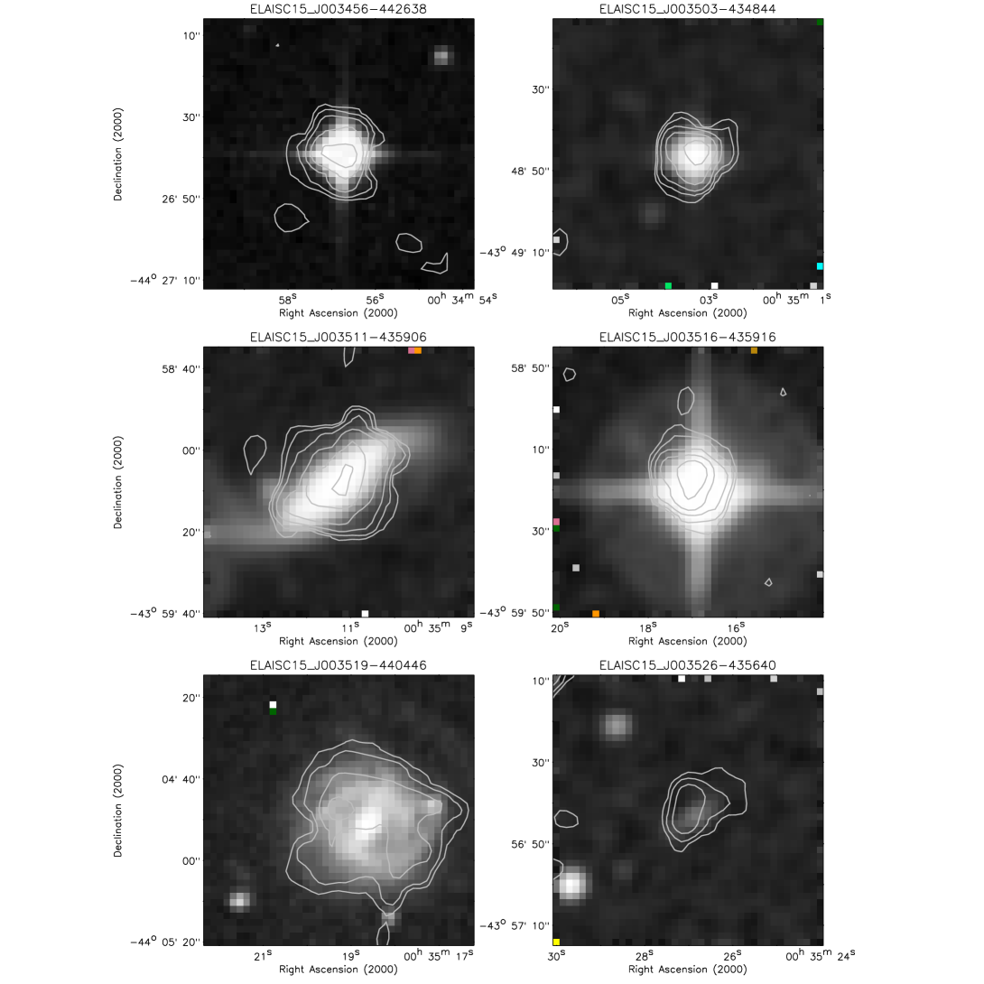
Figure 16: Example of ISOCAM 15 $\mu$m contours superimposed to DSS optical images ($b_{j}$ band). Contour levels of the 15 $\mu$m emission correspond to 0.05, 0.08, 0.15, 0.3, 0.6, 1.2, 2.0, 4.0 mJy / pixel. The size of each image is 1$\times$1 arcmin.

In figure 16 is shown an example of our ISOCAM 15 $\mu$m contour levels superimposed to DSS optical images, after correcting for the systematic offsets computed above. The plot can give an idea of the astrometric accuracy of our catalogue and images. In fact, as clearly visible from the figure, the positions of our sources after offsetting appear as accurate as we estimated from simulations (see above), thus allowing reliable identifications within a few arcseconds or less.

9 Repeated central region, S1$\_$5

The central field of the S1 area, as mentioned in section 4.2, has been observed three times in order to reach a deeper flux limit with respect to the rest of the area and to allow reliability checks on sources.

The reduction of the three observations was carried out in the standard way (see section 4.1) until the stage of map creation. After the creation of the three single raster maps, some particular routines have been applied for combining them and for performing simulations in the combined map.
To obtain a unique combined map from the three single observations, first we have projected all of them on the sky with the same orientation (north-south). The three single rasters have then been corrected for the relative astrometric offsets (see section 8) and then coadded. For the coaddition, each raster map has been weighted, with a weight proportional pixel-by-pixel to its relative “NPIX” map. The combined “NPIX” map was just the pixel-by-pixel sum of each “NPIX” map. The “RMS” distribution over the mosaic map has been obtained with the standard procedure (see 4.1). The average rms value in the central part of the combined S1$\_$5 map is about 0.016 mJy.

Once obtained the combined map, source extraction have been performed in the same way as for the single observation raster maps (see section 4.3). In S1$\_$5 we have detected 93 sources.

To derive the total fluxes from the detected peak fluxes, we have performed the “auto-simulations” (see section 2) for the 93 sources, by injecting point sources into each of the three single fields and then combining the resulting images with the same weight used to coadd the real maps. The total-to-peak ratio found for the simulated sources have then been applied to the peak flux obtained for the real sources to get their total flux, exactly in the same way as we did for the single rasters in the rest of the S1 area.

Total fluxes in the combined map range between 0.57 and $\sim$100 mJy.

9.1 Simulations in S1$\_$5

To perform simulations of the repeated raster we have used and appropriately combined the simulations performed separately on the three single rasters, S1$\_$5, S1$\_$5$\_$B, S1$\_$5$\_$C (section 5). The positions of the sources injected in each of the three individual fields have been chosen in order to simulate the effects caused by the application, in the coaddition phase, of a relative astrometric offset among the rasters. 50 sources for each of the above 5 total fluxes (0.7, 1, 1.4, 2 and 3 mJy) were injected. The “auto-simulations” were performed on the positions found on the combined map.

Figure 17: Output flux after reduction versus output flux due only to sampling effects for simulated sources detected in the combined map S1$\_5$ (dot) and in the main S1 survey (open circle).

In figure 17 the $fs$ and $f0$ peak fluxes of the detected sources are plotted superimposed to the ones found for the simulated sources in the main S1 area. Apart from the deeper detection level, the general trend is the same with a somewhat smaller dispersion. For the 3 mJy input sources the $fs/f0$ observed distribution peaks at 0.82 $\pm$ 0.03 and its width is 0.11, while the corresponding values for single fields simulation are 0.78 $\pm$ 0.03 and 0.18.

Following the same procedure as before we can predict completeness and detection rates also for sources in the combined map.

The results of the simulations have been reported in table 4 and shown in figure 18.

Table 4: Detection rates in the S1$\_5$ combined map

input flux	predicted(mapping)		predicted(map+reduction)		predicted(map+red+incompl)		detected
(mJy)	over injected	(%)	over injected	(%)		(%)		(%)
0.7	47.6/50	95.2	36.2/50	72.4	18.6/50	37.2	14/50	28.0
1.0	50.0/50	100.0	48.4/50	96.8	35.9/50	71.9	36/50	72.0
1.4	50.0/50	100.0	49.9/50	99.9	49.4/50	98.8	49/50	98.0
2.0	50.0/50	100.0	50.0/50	100.0	50.0/50	100.0	50/50	100.0
3.0	50.0/50	100.0	50.0/50	100.0	50.0/50	100.0	50/50	100.0

Figure 18: Percentage of detected sources in simulations of ELAIS S1$\_5$ as a function of the source input flux. As detection threshold we have considered 5$\sigma$. The dashed curve represents the effect of PSF sampling on the detection rate; the dash-dotted curve represents the effect of the LARI method; the solid curve is the total effect on reduced LW3 ELAIS data. The dotted curve is the total detection rate found in S1 (the same as the solid curve plotted in figure 9)

The combination of the three maps does not only reduce the errors in flux determination and increase the fraction of detected sources at faint fluxes, but provides more precise positions in the sky.

Figure 19 shows the distributions of the differences in RA and DEC between the injected and detected positions, while figure 20 shows the dependence of position errors on the signal-to-noise ratio. The widths found for the distributions in RA and DEC for sampling and reduction effect, are 0.92 and 0.85 respectively, smaller than those found for the main survey, 1.17 and 1.27. Considering the dependence of the position errors on the signal-to-noise ratio, the laws found are of the form:

$$\sigma_{s+r}(RA)=0.74+1.59\times e^{-(0.2\times S/N)}$$ (8)

$$\sigma_{s+r}(DEC)=0.54+0.86\times e^{-(0.07\times S/N)}$$ (9)

These law are less steep than those found in the all survey and, as we can see from the figure 20, the values of the positional errors near the limit of the survey (signal-to-noise = 5) are, for both coordinates, less than 1.5^′′.

The combination of the three maps, changing the repetition factor from 2 to 6 for each single pointing image, not only reduces the errors, but also the effects due to mapping.

Figure 19: Distribution of the difference in RA (top) and DEC (bottom) between the injected and the found positions for simulated sources detected in the S1$\_5$ combined map; dashed line: sampling effect; solid line: sampling plus reduction effect.

Figure 20: Positional errors versus signal-to-noise ratio (top: RA; bottom: DEC) for simulated sources detected in the S1$\_5$ combined map. Only errors due to the combined effect of due to mapping and data reduction are plotted as diamonds. The dot-dashed lines represent exponential fits to the error dependency on source signal-to-noise ratio.

10 The Source Catalogue in S1

The final catalogue obtained with our method contains a total of 462 sources detected at 15 $\mu$m (LW3) in the ELAIS region S1. All the sources detected over the whole $2^{\circ}\times 2^{\circ}$ area have signal-to-noise ratio greater than 5. The catalogue reports the source name, the offset-corrected position (right ascension and declination at equinox J2000), the positional accuracy on the final images, the source peak flux (in mJy/pixel), the detection level (signal-to-noise ratio), the total flux and its error (in mJy), the raster name and eventually a note, indicating whether the source is identificated with a star, its flux have been obtained through aperture photometry, etc. In case of extended of very bright sources, the total flux reported in the table is computed by aperture photometry instead of by “auto-simulations”, the latter method providing a correct measurement mainly for unresolved sources. Note that a few sources (belonging to the border part of a raster, overlapping with an adjacent raster) might appear in two different rasters. In this case, the repeated sources have been reported twice in the catalogue and the corresponding additional raster number is quoted in the notes.

As described in section 4.3, before extracting sources on the final maps, we have identified candidate sources inside the pixel histories (flux excesses above the background over the single time-scans greater than 0.7 ADU/gain/s) and on the single calibrated images (all pixels with flux $>0.4$ mJy / pixel), providing 100% reliable lists of sources above these two thresholds. Although there is not a perfect correspondence between these two flux thresholds and total fluxes in the final raster maps (due to flat-fielding, distortions, etc.), we have found that by splitting the S1 catalogue in two (above and below 1 mJy) we can provide a highly reliable catalogue, where all the sources have been checked before extraction and a less reliable but deeper catalogue, where most sources could not be checked with the above criteria. The majority of sources fainter than 1 mJy, in fact, might have flux excesses in the single pixel histories below 0.7 ADU/gain/s and peak fluxes on the single images fainter than 0.4 mJy / pixel, the limits chosen for visual inspection, below which is almost impossible to distinguish a flux excess on the pixel history from local background fluctuations. This does not apply to S1$\_5$, because sources have been extracted on the combination of three single observations, that have been separately checked before the coaddition.

In Tables 5 and 6, the first page (corresponding to the first raster) of the catalogues in S1, respectively above and below 1 mJy, are shown as examples. The full ELAIS S1 + S1$\_5$ catalogues at 15 $\mu$m obtained with Lari method will be available from http://boas5.bo.astro.it/$\sim$elais/catalogues/.

Table 5: The 15 $\mu$m $S\geq 1$ mJy Catalogue in the ELAIS Southern Area S1

Name	RA	DEC	$\sigma$(RA)	$\sigma$(DEC)	Fpeak	$S/N$	Ftot	$\sigma$(Ftot)	raster	notes
	(J2000)	(J2000)	($\prime\prime$)	($\prime\prime$)	(mJy)		(mJy)	(mJy)
ELAISC15$\_$J002818$-$424303	00 28 18.9	$-$42 43 03.8	1.1	1.2	0.362	14.11	2.239	0.555	S1$\_$1	star
ELAISC15$\_$J002831$-$425203	00 28 31.9	$-$42 52 03.6	1.3	1.5	0.192	7.43	1.050	0.302	S1$\_$1
ELAISC15$\_$J002848$-$430658	00 28 48.4	$-$43 06 58.5	1.6	1.6	0.161	6.09	1.000	0.313	S1$\_$1
ELAISC15$\_$J002853$-$425053	00 28 53.9	$-$42 50 53.7	1.7	1.6	0.158	5.62	1.041	0.355	S1$\_$1
ELAISC15$\_$J002857$-$425343	00 28 57.3	$-$42 53 43.2	1.1	1.3	0.323	10.72	2.196	0.590	S1$\_$1	star
ELAISC15$\_$J002904$-$425243	00 29 04.4	$-$42 52 43.1	1.5	1.5	0.175	6.62	1.087	0.322	S1$\_$1
ELAISC15$\_$J002913$-$431717	00 29 13.7	$-$43 17 17.6	1.1	1.1	0.925	37.50	7.648	1.797	S1$\_$1	star
ELAISC15$\_$J002915$-$430333	00 29 15.8	$-$43 03 33.7	1.1	1.3	0.288	12.64	1.855	0.470	S1$\_$1
ELAISC15$\_$J002917$-$423921	00 29 17.4	$-$42 39 21.9	1.4	1.5	0.181	7.10	1.093	0.318	S1$\_$1
ELAISC15$\_$J002930$-$431139	00 29 30.9	$-$43 11 39.9	1.6	1.6	0.157	6.02	1.220	0.379	S1$\_$1
ELAISC15$\_$J002939$-$430625	00 29 39.3	$-$43 06 25.3	1.5	1.5	0.253	6.30	3.400	0.723	S1$\_$1	aper
ELAISC15$\_$J002943$-$423736	00 29 43.7	$-$42 37 36.8	1.8	1.6	0.198	5.47	1.963	0.651	S1$\_$1	star
ELAISC15$\_$J002949$-$430703	00 29 49.1	$-$43 07 03.0	1.3	1.5	0.211	7.60	1.191	0.349	S1$\_$1
ELAISC15$\_$J002956$-$424534	00 29 57.0	$-$42 45 34.7	1.1	1.1	0.704	25.84	4.175	0.989	S1$\_$1	star
ELAISC15$\_$J003014$-$430332	00 30 14.9	$-$43 03 32.8	1.1	1.3	0.302	11.68	2.450	0.624	S1$\_$1
ELAISC15$\_$J003017$-$423721	00 30 17.7	$-$42 37 21.9	1.4	1.5	0.176	7.02	1.470	0.427	S1$\_$1	star
ELAISC15$\_$J003022$-$423657	00 30 22.7	$-$42 36 57.5	1.1	1.1	2.017	77.90	23.000	3.900	S1$\_$1	aper
ELAISC15$\_$J003023$-$424549	00 30 23.3	$-$42 45 49.6	1.1	1.3	0.344	12.96	2.073	0.522	S1$\_$1
ELAISC15$\_$J003025$-$423855	00 30 25.2	$-$42 38 55.2	1.3	1.5	0.189	7.37	1.134	0.329	S1$\_$1
ELAISC15$\_$J003039$-$425348	00 30 39.6	$-$42 53 48.3	1.1	1.3	0.341	13.35	1.980	0.497	S1$\_$1
ELAISC15$\_$J003054$-$430044	00 30 54.4	$-$43 00 44.4	1.2	1.4	0.206	8.11	1.486	0.412	S1$\_$1
ELAISC15$\_$J003101$-$431733	00 31 01.8	$-$43 17 33.1	1.1	1.1	9.746	244.20	103.000	19.200	S1$\_$1	star, aper
ELAISC15$\_$J003104$-$425635	00 31 04.8	$-$42 56 35.1	1.1	1.3	0.289	11.01	2.382	0.620	S1$\_$1
ELAISC15$\_$J003114$-$424228	00 31 14.4	$-$42 42 28.5	1.1	1.1	0.811	30.83	5.968	1.406	S1$\_$1
ELAISC15$\_$J003123$-$430939	00 31 23.6	$-$43 09 39.3	1.5	1.5	0.179	6.49	1.032	0.318	S1$\_$1
ELAISC15$\_$J003133$-$424445	00 31 33.5	$-$42 44 45.7	1.1	1.2	0.571	21.42	4.318	1.034	S1$\_$1
ELAISC15$\_$J003137$-$425844	00 31 37.9	$-$42 58 44.3	1.3	1.5	0.188	7.34	1.107	0.316	S1$\_$1
ELAISC15$\_$J003142$-$425642	00 31 42.9	$-$42 56 42.2	1.8	1.6	0.150	5.51	1.188	0.389	S1$\_$1
ELAISC15$\_$J003151$-$431046	00 31 51.0	$-$43 10 46.6	1.4	1.5	0.163	6.64	1.167	0.344	S1$\_$1
ELAISC15$\_$J003151$-$424540	00 31 51.5	$-$42 45 40.7	1.9	1.6	0.141	5.22	1.004	0.335	S1$\_$1
ELAISC15$\_$J003216$-$430432	00 32 16.4	$-$43 04 32.4	1.1	1.1	2.025	77.09	12.136	2.820	S1$\_$1
ELAISC15$\_$J003223$-$430546	00 32 23.9	$-$43 05 46.1	1.3	1.5	0.197	7.90	1.259	0.352	S1$\_$1
ELAISC15$\_$J003232$-$431306	00 32 32.6	$-$43 13 06.6	2.0	1.6	0.188	5.00	1.085	0.367	S1$\_$1
ELAISC15$\_$J003233$-$430632	00 32 33.1	$-$43 06 32.2	1.4	1.5	0.190	6.64	1.663	0.527	S1$\_$1

Table 6: The 15 $\mu$m $S<1$ mJy Catalogue in the ELAIS Southern Area S1

Name	RA	DEC	$\sigma$(RA)	$\sigma$(DEC)	Fpeak	$S/N$	Ftot	$\sigma$(Ftot)	raster	notes
	(J2000)	(J2000)	($\prime\prime$)	($\prime\prime$)	(mJy)		(mJy)	(mJy)
ELAISC15$\_$J002929$-$430651	00 29 29.8	$-$43 06 51.5	2.0	1.6	0.111	5.13	0.666	0.238	S1$\_$1
ELAISC15$\_$J002938$-$424123	00 29 38.6	$-$42 41 23.0	1.5	1.5	0.163	6.48	0.971	0.292	S1$\_$1
ELAISC15$\_$J003128$-$430747	00 31 28.9	$-$43 07 47.2	1.9	1.6	0.119	5.25	0.736	0.278	S1$\_$1
ELAISC15$\_$J003144$-$425826	00 31 44.9	$-$42 58 26.8	1.9	1.6	0.136	5.21	0.768	0.257	S1$\_$1
ELAISC15$\_$J003147$-$423548	00 31 47.3	$-$42 35 48.8	1.6	1.6	0.154	6.01	0.836	0.262	S1$\_$1
ELAISC15$\_$J003147$-$423523	00 31 47.7	$-$42 35 23.2	1.5	1.5	0.163	6.46	0.970	0.289	S1$\_$1
ELAISC15$\_$J003214$-$425339	00 32 14.4	$-$42 53 39.6	1.4	1.5	0.173	6.87	0.944	0.281	S1$\_$1	star
ELAISC15$\_$J003218$-$430542	00 32 18.3	$-$43 05 42.3	1.8	1.6	0.152	5.42	0.821	0.291	S1$\_$1
ELAISC15$\_$J003221$-$430020	00 32 21.7	$-$43 00 20.3	2.0	1.6	0.128	5.04	0.868	0.298	S1$\_$1
ELAISC15$\_$J003225$-$430712	00 32 25.8	$-$43 07 12.3	2.0	1.6	0.127	5.00	0.971	0.332	S1$\_$1
ELAISC15$\_$J003228$-$430758	00 32 28.0	$-$43 07 58.6	1.9	1.6	0.135	5.27	0.826	0.277	S1$\_$1
ELAISC15$\_$J003233$-$431304	00 32 33.4	$-$43 13 04.6	1.4	1.5	0.232	6.79	0.981	0.286	S1$\_$1

11 Conclusions

A new data reduction technique (the Lari method) has been successfully applied to the 15 $\mu$m ISOCAM observations of one of the four main ELAIS fields (S1). This technique, based on the existence of two different time-scales in ISOCAM transients, was particularly efficient in overcoming the main problems affecting the ISOCAM LW data and in detecting faint sources. Its application to the southern ELAIS field has produced a catalogue of 462 sources, detected above the 5 $\sigma$ threshold over an area of about 4 square degrees. The integrated fluxes of these sources cover the range 0.5 - 100 mJy, filling the existing gap between the Deep ISOCAM Surveys and the Faint IRAS Survey. The completeness and photometry accuracy of our catalogue have been tested through accurate simulations performed at different flux levels. The results of these simulations showed that our catalogue is highly reliable and $>98.5$% complete at 3 mJy. The completeness, due either to the mapping effects or to the data reduction method, then decreases at fainter fluxes. The positional accuracy, estimated with simulations, resulted to be about 1 arcsec in both right ascension and declination for signal-to-noise ratios $>7$, while it increases to $\sim 2$ and 1.6 at signal-to-noise ratios close to the survey threshold (5), respectively for right ascension and declination. The photometric accuracy of our data reduction has also been tested using the stars of the field, comparing the measured fluxes with the ones predicted by the relation calibrated on IRAS data by Aussel & Alexander (2000). Our fluxes resulted well consistent with the predicted ones over a large range of fluxes, since these stars go from 0.85 mJy to 135 mJy in LW3.

In a forthcoming paper (Gruppioni, Lari, Pozzi et al. 2001) we will present the source counts obtained from this survey in the crucial uncovered flux range 0.45 – 100 mJy, dividing the Deep/Ultra-Deep ISOCAM Surveys from the fainter IRAS Surveys.

Appendix A Lari Model Description

The process is governed by two differential equations, one for each charge reservoir, of the form:

$$\frac{dQ}{dt}=eI-aQ^{2}$$ (10)

where $I$ is the incident flux of photons, $e$ is the efficiency of the process feeding the component and $a$ is a time constant which depends on the detector pixel-size. Note that $e$ and $a$ assume different values for the two components: $a($breve) $>a($lunga) and $e($breve) $>e($lunga).

We have not attempted to model $I$ and $e$ for glitches. In principle, glitches could be described by the physics of ionising particles. However their effect strongly depends on the nature and energy of the incident cosmic particle. For example, high energy incident cosmic rays could produce saturation on the detector, thus causing the parameter $e$ to depend on the values of $I$ and $Q$ . For simplicity, we have neglected this effect in our model, considering both $e$ and $a$ as constants.

Our model is completely conservative (no decay of the accumulated charges is considered, except toward the contacts) and homogeneous (the charge reservoir involves all the detector parts that do not contribute to polarising the contacts). In fact, at stabilisation we have $aQ^{2}=eI$ and $S=I$ ($S$ being the signal), while generally $I=S+\Delta Q/\Delta t$. The quantity $-aQ^{2}$ in the accumulated charge equation is exactly the same amount of charge which that component feeds the contacts with.

Considering charges as fluxes in ADUs ($q=Q/\Delta t$), we have:

$$\Delta t~{}\frac{dq_{1}}{dt}=e_{1}I-a_{1}\Delta t^{2}~{}q_{1}^{2}$$ (11)

for the breve component. Integrating over an observation integration time $\Delta t$ (with $I=$ constant):

$$\Delta q_{1}=e_{1}I-a_{1}\Delta t^{2}<q_{1}^{2}>$$ (12)

and

$$\Delta t~{}\frac{dq_{2}}{dt}=e_{2}I-a_{2}\Delta t^{2}~{}q_{2}^{2}$$ (13)

for the lunga component, which integrated over an integation time becomes

$$\Delta q_{2}=e_{2}I-a_{2}\Delta t^{2}<q_{2}^{2}>.$$ (14)

We then have

$$S(obs.~{}signal)=e_{0}I+a_{1}\Delta t^{2}<q_{1}^{2}>+a_{2}\Delta t^{2}<q_{2}^{2}>$$ (15)

where $e_{0}+e_{1}+e_{2}=1$

The two differential equations are of Riccati type, which, for $I=constant$ have a general analytical solution:

$${q(t)}=A\times\frac{((A+q(0))~{}e^{bt}-(A-q(0)))}{((A+q(0))~{}e^{bt}+(A-q(0))}$$ (16)

where $q$ can be either $q_{1}$ or $q_{2}$. $A$ represents the asymptotic value for $q$ ($A=\frac{\sqrt{eI/a}}{\Delta t}$), while $b$ ($=2\sqrt{eIa}$) is the inverse of the time–scale at stabilisation. Note that the time–scale in this model is inversely proportional to the square root of the (constant) incident flux (at stabilisation only!), while the observed flux $S$ tends to $I$ as $t$ tends to infinity.

In our code we make use also of an approximate equation with finite difference values to obtain valid solutions also for the general case of variable $I$:

$$(q(t+\Delta t)-q(t))=eI(t)-a\Delta t^{2}q(t+\Delta t)q(t)$$ (17)

where $q$ is either $q_{1}$ or $q_{2}$, $e$ is either $e_{1}$ or $e_{2}$, $a$ is either $e_{1}$ or $e_{2}$, respectively for the breve and for the lunga components. $q(t)$ and $q(t+\Delta t)$ are the charges that are accumulated respectively at the beginning and at the end of and integration. $I(t)$ is the average intensity over the whole integration.

The error we commit by use of this second-order approximation instead of the exact equation is less than 1%, so this can be considered a good approximation. The same kind of approximation is used in other parts of our code when calculating derivatives.

In equation 15 the observed flux is the flux subtracted by the dark current. In dark observations ‘glitch’ transients show as ‘faders’ and ‘dippers’, the latter having time-scales larger than the integration time, but not infinite (as the model requires). Thus, both lunga and breve charge productions are fed also by the thermal component of the dark current. This effect might be important when the photon flux is small. It is very difficult to estimate this extra source of transient signal and, since we could not find any documentation on ISOCAM thermal dark current measurements, we tried to estimate it from the data. We have thus associated the thermal dark current to the minimum amount of extra signal that is needed in order to keep the parameter $e_{2}$ below the value of the lunga fraction ($\simeq 0.1$, implying that dippers cannot exceed one-tenth of the sky background counts).

By giving the name ‘offset’ to the thermal feeding, equations 12, 14 and 15 become:

$$\Delta q_{1}=e_{1}(I+offset)-a_{1}\Delta t^{2}<q_{1}^{2}>$$ (18)

$$\Delta q_{2}=e_{1}(I+offset)-a_{2}\Delta t^{2}<q_{2}^{2}>$$ (19)

$$S(obs.~{}signal)+offset=$$ (20)

$$e_{0}(I+offset)+a_{1}\Delta t^{2}<q_{1}^{2}>+a_{2}\Delta t^{2}<q_{2}^{2}>$$

In practice, these two equations can be solved by successive iterations, provided that $q_{1/2}(0)$, $e_{1/2}$ and $a_{1/2}$ are known. Estimates for these parameters, characterising each pixel, can be obtained by minimising the $\chi^{2}$ estimator, under the condition of having a constant incident flux at each raster position. In this model, all the past history of each pixel is contained in the intial charge, as long as there is no other source of electrons (eg from the surrounding pixels or from longer time relaxation processes inside the pixel).

References

- [Akin(1970)] Akin H. and Colton R.R., 1970, Statistical Methods, Fifth Barnes & Nobles Books Edition
- [Alexander(2000)] Alexander A. & Aussel H., in D. Lemke, M. Stickel and K. Wilke eds., ISO Surveys of a Dusty Universe, Springer Lecture Notes of Physics Series, p. 113
- [Aussel(1999)] Aussel H., Cesarsky C.J., Elbaz D. and Starck J.-L., 1999, A&A, 342, 313
- [Cesarsky(1996)] Cesarsky C.J., Abergel A., Agnèsel P. et al., 1996, A&A, 315, L32
- [Elbaz(1999)] Elbaz D., Cesarsky C. J., Fadda D., Aussel H., Désert F.X., Franceschini A., Flores H., Harwit M., Puget J.-L., Starck J.-L., Clements D.L., Danese L., Koo D.C. and Mandolesi R., 1999, A&A, 351, L37
- [Flores(1999)] Flores H., Hammer F., Thuan T.X., Césarsky C., Desert F.X., Omont A., Lilly S.J., Eales S., Crampton D. and Le F vre O., 1999, ApJ, 517, 148
- [Gruppioni(1999)] Gruppioni C., Ciliegi P., Rowan–Robinson M., Cram L., Hopkins A., Cesarsky C., Danese L., Franceschini A., Genzel R., Lawrence A., Lemke D., McMahon R.G., Miley G., Oliver S., Puget J.-L. and Rocca-Volmerange B., 1999, MNRAS, 305, 297
- [Gruppioni(2000)] Gruppioni C., Lari C., Pozzi F., Zamorani G. and Franceschini A., 2001, MNRAS, submitted
- [Hog(2000)] Hög E., Fabricius C., Makarov V.V., Bastian U., Schwekendiek P., Wicenec A., Urban S., Corbin T. and Wycoff G., 2000, A&A, 357, 367
- [Kessler(1996)] Kessler M., Steinz J., Anderegg M. et al., 1996, A&A, 315, L27
- [Lejeune(1998)] Lejeune T. and Cuisinier F. and Buser R., 1998, A&ASS, 130, 65
- [Monet(1998)] Monet D.G., 1998, AAS Meeting, 193, p. 120.03
- [Okumura(1998)] Okumura K., 1998, ISOCAM PSF Report, available at http://www.iso.vilspa.esa.es/users/expllib/CAMlist.html
- [Okumura(2000)] Okumura K., 2000, ISOCAM Field Distortion Report, available at http://www.iso.vilspa.esa.es/users/expllib/CAMlist.html
- [Oliver(2000)] Oliver S., Rowan–Robinson M., Alexander D.M. et al., 2000, MNRAS, 316, 749
- [Omont(1999)] Omont A., Ganesh S., Alard C., Blommaert J.A.D., Caillaud B. et al., 1999, A&A, 348, 755
- [Schlegel(1998)] Schlegel D.J., Finkbeiner D.P. and Davis M., 1998, ApJ, 500, 525
- [Serjeant(2000)] Serjeant S., Oliver S., Rowan–Robinson M. et al., 2000, MNRAS, in press
- [Starck(1999)] Starck J.-L., Aussel H., Elbaz D., Fadda D. and Cesarsky C., 1999, A&AS, 138,365